1 Introduction
Extreme and rogue waves are a potentially life-threatening and catastrophic phenomenon (Dysthe, Krogstad & Müller Reference Dysthe, Krogstad and Müller2008), and the need to study their statistics and driving mechanisms is clear. Oceanic rogue or freak waves are generally defined as waves for which the ratio of wave height (
 $H$
) or crest height (
 $\unicode[STIX]{x1D702}_{c}$
) to significant wave height (
 $H_{s}$
) exceeds a certain value (Kharif & Pelinovsky Reference Kharif and Pelinovsky2003), for example
 $H/H_{s}>2.0$
or
 $\unicode[STIX]{x1D702}_{c}/H_{s}>1.25$
, although several other definitions exist (e.g. Dean Reference Dean, Trum and Gudmestad1990). Kurtosis can be used as a measure of the relative importance of nonlinearities (Janssen Reference Janssen2003) and hence the probability of extreme waves, while the skewness describes the importance of the second-order bound nonlinearities (Fedele et al.
Reference Fedele, Brennan, Ponce De León, Dudley and Dias2016). Bi-modal or crossing seas, when there are two distinctive peaks in the directional spectra, can be observed in general sea states (e.g. Semedo et al.
Reference Semedo, Sušelj, Rutgersson and Sterl2011) as well as extreme seas such as tropical cyclones (Mori Reference Mori2012). Mixed sea states, in which there are two or more distinct spectral peaks, have been shown to occur in the North Sea with a probability of occurrence of around 25 % (Boukhanovsky, Lopatoukhin & Guedes Soares Reference Boukhanovsky, Lopatoukhin and Guedes Soares2007). Crossing seas alter the statistical structure of surface waves and several marine accidents involving large or rogue waves are known to have occurred in crossing seas (Toffoli et al.
Reference Toffoli, Lefevre, Bitner-Gregersen and Monbaliu2005) including the well-known Draupner wave (Onorato, Osborne & Serio Reference Onorato, Osborne and Serio2006; Mcallister et al.
Reference Mcallister, Draycott, Adcock, Taylor and van den Bremer2019). In directionally spread crossing seas much of the recent research work on wave statistical development and rogue waves is based on numerical studies (e.g. Bitner-Gregersen & Toffoli Reference Bitner-Gregersen and Toffoli2014; Trulsen et al.
Reference Trulsen, Nieto Borge, Gramstad, Aouf and Lefèvre2015; Gramstad et al.
Reference Gramstad, Bitner-Gregersen, Trulsen and Nieto Borge2018). The present study aims to extend previous experimental studies by focusing on two crossing directionally spread systems and to test whether empirical models and results from single-component seas can be applied or extended to crossing or bi-modal seas.
Third-order quasi-resonant interactions and associated modulational instabilities can cause the statistics of weakly nonlinear gravity waves to significantly differ from the Gaussian structure of linear seas (Janssen Reference Janssen2003; Fedele Reference Fedele2008; Onorato et al. Reference Onorato2009; Shemer & Sergeeva Reference Shemer and Sergeeva2009; Toffoli et al. Reference Toffoli, Gramstad, Trulsen, Monbaliu, Bitner-Gregersen and Onorato2010a ; Xiao et al. Reference Xiao, Liu, Wu and Yue2013). This mechanism is usually associated with deep water, but is also present in intermediate-depth water (Toffoli et al. Reference Toffoli, Fernandez, Monbaliu, Benoit, Gagnaire-Renou, Lefevre, Cavaleri, Proment, Pakozdi and Stansberg2013). For narrow-banded waves, the importance of modulational instabilities can be described by the Benjamin–Feir index (BFI) (Benjamin & Feir Reference Benjamin and Feir1967; Janssen Reference Janssen2003):
 $$\begin{eqnarray}\text{BFI}=\frac{\sqrt{2}\unicode[STIX]{x1D700}}{\unicode[STIX]{x1D6FF}_{\unicode[STIX]{x1D714}}},\end{eqnarray}$$
where the frequency spectrum bandwidth
 $\unicode[STIX]{x1D6FF}_{\unicode[STIX]{x1D714}}=\unicode[STIX]{x1D70E}_{\unicode[STIX]{x1D714}}/\unicode[STIX]{x1D714}_{p}$
,
 $\unicode[STIX]{x1D70E}_{\unicode[STIX]{x1D714}}$
is the standard deviation of the frequency spectrum,
 $\unicode[STIX]{x1D714}_{p}$
is the peak angular frequency and
 $\unicode[STIX]{x1D700}$
is the wave steepness. The wave steepness is defined here as
 $\unicode[STIX]{x1D700}=\sqrt{m_{0}}k_{p}$
, where the
 $m_{0}$
is the zeroth-order moment of the variance density spectrum and
 $k_{p}$
is the wavenumber at the spectral peak derived from a spectral analysis of the time series with subsequent application of the linear dispersion relationship.
Unidirectional (long-crested) seas where the dissipation is negligible and the wave steepness is small and thus where quasi-resonant interactions are effective in the reshaping of the wave spectrum are rare. Ocean waves are typically multi-directional (short-crested) and energy can spread directionally. Experimental (Onorato et al. Reference Onorato2009; Waseda, Kinoshita & Tamura Reference Waseda, Kinoshita and Tamura2009) and numerical (Mori & Janssen Reference Mori and Janssen2006; Gibson & Swan Reference Gibson and Swan2007; Gramstad & Trulsen Reference Gramstad and Trulsen2007; Fedele & Tayfun Reference Fedele and Tayfun2009) investigations have found that as the directionality in the sea increases, the quasi-resonant effects decrease. Although modulational instability-like resonant or quasi-resonant interactions accelerate the probability of rogue waves, recent analysis of field data (Fedele et al. Reference Fedele, Brennan, Ponce De León, Dudley and Dias2016) suggests that second-order bound mode effects enhance the directional and dispersive interference that is the main driver for observed rogue wave activity in the ocean.
A number of studies have shown that crossing seas differ significantly from unimodal seas. Onorato et al. (Reference Onorato, Osborne and Serio2006) investigated simplified crossing seas using the nonlinear Schrödinger equation. They found that introducing a second wave system can increase the instability growth rate and increase the size of the unstable region. Again using the nonlinear Schrödinger equation, Shukla et al. (Reference Shukla, Kourakis, Eliasson, Marklund and Stenflo2006) found that two crossing long-crested wave trains can form large-amplitude wave groups even when the individual wave trains are modulationally stable; and Grönlund, Eliasson & Marklund (Reference Grönlund, Eliasson and Marklund2009) found that two-wave coupled systems show increased nonlinear focusing and decreased time to develop large waves compared to a non-coupled system. Using the nonlinear Schrödinger equation, Gramstad & Trulsen (Reference Gramstad and Trulsen2010) found the addition of a swell wave system slightly increases the number of rogue waves in a short-crested wind sea.
Mori, Onorato & Janssen (Reference Mori, Onorato and Janssen2011) suggest an extension of the BFI, the two-dimensional BFI or
 $\text{BFI}_{2D}$
, for waves with significant directional spread. This is based on the BFI and the frequency spectrum bandwidth
 $R$
, which is a measure of the angular width with respect to frequency:
 $$\begin{eqnarray}\displaystyle & \displaystyle R=\frac{\unicode[STIX]{x1D6FF}_{\unicode[STIX]{x1D703}}^{2}}{2\unicode[STIX]{x1D6FF}_{\unicode[STIX]{x1D714}}^{2}}, & \displaystyle\end{eqnarray}$$
 $$\begin{eqnarray}\displaystyle & \displaystyle \text{BFI}_{2D}={\displaystyle \frac{\text{BFI}}{\sqrt{1+\unicode[STIX]{x1D6FC}_{2}R}}}={\displaystyle \frac{\sqrt{2}\unicode[STIX]{x1D700}}{\sqrt{\unicode[STIX]{x1D6FF}_{\unicode[STIX]{x1D714}}^{2}+\unicode[STIX]{x1D6FC}_{2}\unicode[STIX]{x1D6FF}_{\unicode[STIX]{x1D703}}^{2}/2}}}, & \displaystyle\end{eqnarray}$$
where the directional bandwidth
 $\unicode[STIX]{x1D6FF}_{\unicode[STIX]{x1D703}}$
is the standard deviation of the directional spectrum (in radians) and the constant
 $\unicode[STIX]{x1D6FC}_{2}$
is empirically determined in Mori et al. (Reference Mori, Onorato and Janssen2011) as
 $\unicode[STIX]{x1D6FC}_{2}=7.10$
in a stationary, homogeneous and weakly nonlinear unimodal directional sea state.
Kurtosis gives an indication of the nonlinearity of the spectrum. Assuming a mean of zero for the surface elevation
 $\unicode[STIX]{x1D702}$
, kurtosis
 $\unicode[STIX]{x1D707}_{4}$
is defined as the fourth moment around the mean
 $\langle \unicode[STIX]{x1D702}^{4}\rangle$
divided by the square of the average surface elevation variance
 $\langle \unicode[STIX]{x1D702}^{2}\rangle$
(which is here equal to the zeroth-order moment of the variance density spectrum,
 $\langle \unicode[STIX]{x1D702}^{2}\rangle =m_{0}$
):
 $$\begin{eqnarray}\text{kurtosis}=\unicode[STIX]{x1D707}_{4}=\frac{\langle \unicode[STIX]{x1D702}^{4}\rangle }{\langle \unicode[STIX]{x1D702}^{2}\rangle ^{2}}.\end{eqnarray}$$
For a Gaussian random wave field, the kurtosis is equal to 3. The excess kurtosis is
 $\unicode[STIX]{x1D707}_{4}-3$
. Excess kurtosis comprises a dynamic component due to nonlinear wave–wave interactions (Janssen Reference Janssen2003) and a bound contribution induced by the characteristic crest–trough asymmetry of ocean waves. In the narrow-banded approximation, the kurtosis accounting for the contribution to deviations from Gaussian statistics by second- and third-order bound nonlinearities (Fedele et al.
Reference Fedele, Brennan, Ponce De León, Dudley and Dias2016) can be expressed as a function of wave steepness (Mori & Janssen Reference Mori and Janssen2006):
 $$\begin{eqnarray}\unicode[STIX]{x1D707}_{4}^{bound}=3+24\left(k_{p}\sqrt{\langle \unicode[STIX]{x1D702}^{2}\rangle }\right)^{2}=3+24\unicode[STIX]{x1D700}^{2}.\end{eqnarray}$$
For unidirectional narrow-band waves the dynamic kurtosis due to the third-order quasi-resonant interactions is obtained as (Mori & Janssen Reference Mori and Janssen2006)
 $$\begin{eqnarray}\unicode[STIX]{x1D707}_{4}^{dyn}=\frac{\langle \unicode[STIX]{x1D702}^{4}\rangle }{\langle \unicode[STIX]{x1D702}^{2}\rangle ^{2}}=3+\frac{\unicode[STIX]{x03C0}}{\sqrt{3}}\left(\frac{\sqrt{2}k_{p}\sqrt{\langle \unicode[STIX]{x1D702}^{2}\rangle }}{\unicode[STIX]{x1D70E}_{\unicode[STIX]{x1D714}}/\unicode[STIX]{x1D714}_{p}}\right)^{2}=3+\frac{\unicode[STIX]{x03C0}}{\sqrt{3}}\text{BFI}^{2}.\end{eqnarray}$$
Toffoli et al. (Reference Toffoli, Bitner-Gregersen, Osborne, Serio, Monbaliu and Onorato2011) note that the statistical uncertainty in the kurtosis is high, requiring large datasets to achieve a reliable result. Gramstad et al. (Reference Gramstad, Bitner-Gregersen, Trulsen and Nieto Borge2018, appendix) find in a numerical study that the kurtosis approaches the final value after around 180 waves, while Stansberg (Reference Stansberg1994) states that 1500 random waves are sufficient for kurtosis stability. A strong link between increasing kurtosis and increasing freak wave occurrence was established by Mori & Janssen (Reference Mori and Janssen2006) and a theoretical analysis validated against laboratory data by Mori et al. (Reference Mori, Onorato and Janssen2011) found that as directional dispersion increases so the kurtosis decreases.
Bi-modal long-crested waves (i.e. two distinct long-crested components crossing each other) showed reduced kurtosis and rogue wave activity compared to unimodal waves in numerical studies by Støle-Hentschel et al. (Reference Støle-Hentschel, Trulsen, Rye and Raustøl2018). For more complex sea states involving bi-modal short-crested seas, an experimental study by Petrova & Guedes Soares (Reference Petrova and Guedes Soares2009) investigated the effect of different ratios of wind sea to swell sea at three crossing angles on the kurtosis in intermediate-depth water. In wind-sea-dominated conditions they found that the kurtosis was higher than for swell-dominated conditions. Hindcast simulations of the Draupner wave have found no significant third-order effects (Brennan, Dudley & Dias Reference Brennan, Dudley and Dias2018), while Trulsen et al. (Reference Trulsen, Nieto Borge, Gramstad, Aouf and Lefèvre2015) found no evidence that nonlinear interactions between two crossing wave systems impacted kurtosis or maximum wave height in the Prestige accident.
Experimental studies (Toffoli et al.
Reference Toffoli, Bitner-Gregersen, Osborne, Serio, Monbaliu and Onorato2011; Sabatino & Serio Reference Sabatino and Serio2015) suggest that the kurtosis increases to a maximum between
 $40^{\circ }$
and
 $60^{\circ }$
crossing angle. A more recent numerical study reported in Gramstad et al. (Reference Gramstad, Bitner-Gregersen, Trulsen and Nieto Borge2018) found a peak in kurtosis at large and small crossing angles for broad-banded crossing seas, while crest height was found to be nearly independent of crossing angle. In numerical studies using directionally spread crossing seas, Bitner-Gregersen & Toffoli (Reference Bitner-Gregersen and Toffoli2014) found that the energy and frequency of the wave systems were the most important factors in determining rogue wave probability, but the maximum wave height was affected by crossing angle with a peak around
 $40^{\circ }$
.
The directional spreading affects the distribution of wave heights and wave crests. If the directional spectrum is narrow enough, the wave height distribution will follow the (first-order) Rayleigh distribution (Longuet-Higgins Reference Longuet-Higgins1980); however the Rayleigh distribution tends to over-predict the higher wave heights in experimental data. Forristall (Reference Forristall1978) developed an empirical fit to a Weibull distribution to improve on the Rayleigh distribution for large wave heights. In order to account for differences between observations and Rayleigh distributions, Mori & Janssen (Reference Mori and Janssen2006) included nonlinear effects in the wave height distribution using an Edgeworth series; the resulting distribution has been named the modified Edgeworth–Rayleigh (MER) distribution and describes the deviation from linear statistics under the hypothesis of a narrow-banded, weakly nonlinear wave train.
Qualitatively the sharpening of wave crests is the most obvious manifestation of nonlinearity in the ocean. Under the hypothesis of deep water and narrow-banded waves, Tayfun (Reference Tayfun1980) derived a second-order wave crest distribution (given below in (2.11)). The Tayfun formula enhances the tail of the Rayleigh distribution, especially if the wave steepness is large. The assumption is that the departure from the Rayleigh distribution is due to the presence of bound (phase-locked) modes and not due to the dynamics of free waves; the Stokes wave nonlinearity is accounted for, but the nonlinear interactions among free wave components are not. The statistics of long-crested waves are different from those of short-crested waves, but both long-crested and short-crested waves show a trend to reach crest heights above the second-order distribution (Buchner et al. Reference Buchner, Forristall, Ewans, Christou and Henning2011), while the wave heights are generally well described by first-order distributions.
There has been some significant recent work on rogue wave occurrence in directionally spread crossing seas, but as much of the work is based on numerical studies it is clear that further analyses based on experimental data are required. The work reported here is based on an experimental programme carried out to study wave dynamics and the statistical properties of extreme and rogue waves in directionally spread and crossing sea conditions. The aim of this paper is to examine the statistical properties of extreme and rogue wave activity in crossing directional seas with particular focus on the kurtosis. The specific objectives are firstly to investigate the effect of changing crossing angle, directional spread and component frequency on the kurtosis in directionally spread crossing seas; secondly to investigate the extent to which the most widely used statistical distributions of wave heights and crest heights describe the measured distributions in directionally spread crossing seas; and thirdly to test an empirical estimate of the kurtosis from the
 $\text{BFI}_{2D}$
in directionally spread crossing seas. Following this introduction is a method section describing the test procedure and analysis methods, followed by a results section and analysis of exceedance probabilities and kurtosis. That analysis is followed by a discussion and conclusions.
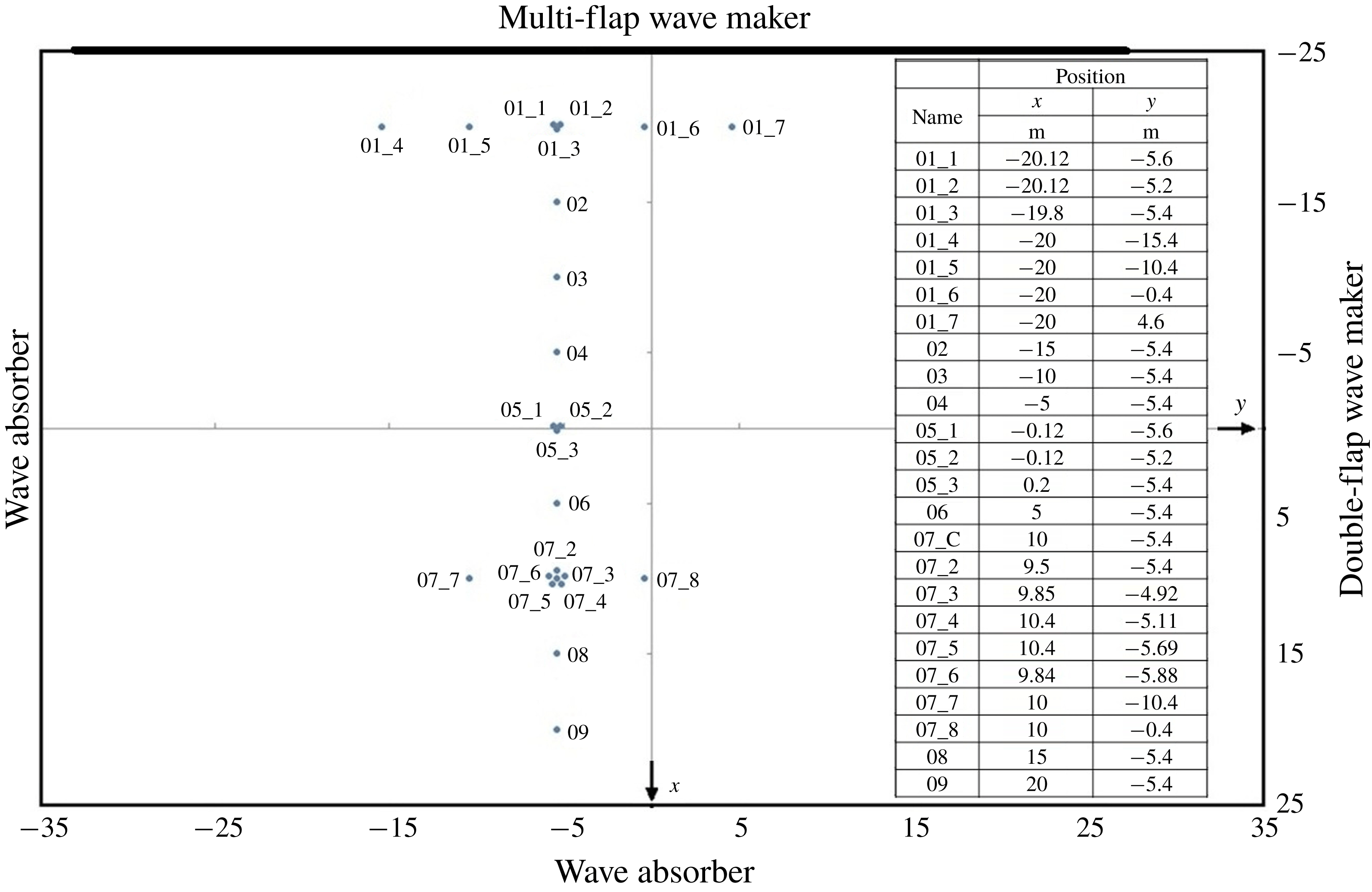
Positions and naming convention for the wave gauges in the Marintek Ocean Basin in Trondheim, Norway.

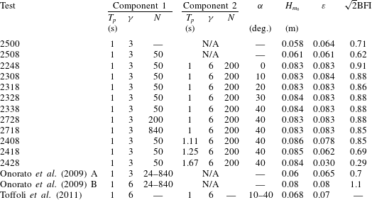
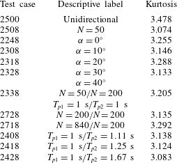
Selected irregular wave tests at Marintek Ocean Basin. All tests use a JONSWAP spectrum. All data are input (requested) values except
 $H_{m_{0}}$
which is measured at wave gauge
 $01_{3}$
. Also shown are details of two previous experiments at Marintek.

2 Method
2.1 Experimental methodology
The experimental tests were carried out at the Marintek Ocean Basin Laboratory in Trondheim, Norway. The Ocean Basin has a water surface area of 50 m by 80 m including the side wave absorber, with the full depth of 3 m extending over an area of 50 m by 70 m as shown in figure 1. The waves were created by a multi-flap wave maker on one of the long sides with 144 individually controlled hinged-type paddles. The far end and right-hand side have wave absorption systems, while the left-hand side has a double-flap wave maker which was switched off during the tests.
The Ocean Basin was instrumented with 24 twin-wire resistance-type wave gauges measuring surface elevation at 100 Hz. The positions of the gauges are shown in figure 1. The gauges are offset from the centreline of the tank by 5.4 m to reduce the presence of reflections from the double-flap wave maker in the measurements. There are three arrays of probes designed to measure directionality in the wave field: probes
 $01_{1}$
,
 $01_{2}$
and
 $01_{3}$
and probes
 $05_{1}$
,
 $05_{2}$
and
 $05_{3}$
are laid out in two equilateral triangles with edges of 0.4 m. Probes
 $07_{2}$
to
 $07_{6}$
are arranged in a pentagon with a diameter of 1 m with probe
 $07_{C}$
in the centre. The rightmost nine paddles (
 $x\approx 30{-}35~\text{m}$
) on the multi-flap wave maker were switched off to reduce reflections from the double-flap wave maker. To reduce the buildup of reflected waves and to reduce any cross-tank seiching the tests were limited to 23 min long with at least 15 min settling time between tests. Frequency spectrum analysis showed that there was some limited seiching detectable. Directional analysis showed that the spectral energy contained in the reflections is below 5 % of the total energy. In general the results presented in this paper use data from nine probes directly down the centreline of the tank (
 $y=-5.4~\text{m}$
) using
 $7_{C}$
at position 7 rather than
 $7_{2}$
. The only exception to this is the directional analysis which uses the five probes in the pentagon array and probe
 $7_{C}$
.
The test conditions considered in this paper are listed in table 1. The experimental design follows on from two previous experiments at the Marintek Ocean Basin: firstly that of Onorato et al. (Reference Onorato2009) examining the statistics of directionally spread unimodal seas and secondly that of Toffoli et al. (Reference Toffoli, Bitner-Gregersen, Osborne, Serio, Monbaliu and Onorato2011) examining kurtosis with two crossing unidirectional wave trains. In table 1 the BFI is multiplied by
 $\sqrt{2}$
to allow easy comparison to Onorato et al. (Reference Onorato2009). The requested input significant wave height
 $H_{m_{0}}$
for each component was 0.058 m, which resulted in a measured significant wave height of around 0.08 m for two-component tests and close to 0.058 m for single-component tests. Throughout this paper
 $H_{m_{0}}$
is measured at wave gauge
 $01_{3}$
and is calculated from the zeroth-order moment of the variance density spectrum
 $m_{0}$
as
 $H_{m_{0}}=4\sqrt{m_{0}}$
. Parameter
 $H_{m_{0}}$
is referred to as the significant wave height although the original definition of significant wave height is based on the mean of the highest
 $1/3$
of waves in a wave record
 $H_{1/3}$
. For the present tests the difference between
 $H_{m_{0}}$
and
 $H_{1/3}$
is up to 4 %. Previous studies (Toffoli et al.
Reference Toffoli, Onorato, Bitner-Gregersen and Monbaliu2010b
; Sabatino & Serio Reference Sabatino and Serio2015) have found that rogue wave activity is increased around
 $40^{\circ }$
crossing angle, so tests of the effects of component frequency and directional spread are performed at this crossing angle.
All tests except test number 2500 were repeated four times to give long enough time series for robust statistical analysis. The first three minutes of each test were removed prior to analysis giving around 80 min of data at each condition, or roughly 4800 waves. The analysis reported in this paper is all conducted on the full combined 80 min tests, again with the exception of test 2500, so the roughly 4800 waves used in the present experiments should give a stable value. An analysis of the kurtosis showed that above 3000 waves the kurtosis approaches a stable value – above 3000 waves the standard deviation is below 0.3 % of the mean value for all tests at all nine locations down the tank.
For all the tests listed except tests 2500 and 2508 there were two spectral wave components requested. Both components use a JONSWAP spectrum, component 1 with
 $\unicode[STIX]{x1D6FE}=3$
and component 2 with
 $\unicode[STIX]{x1D6FE}=6$
. For component 2 the spreading factor is set to
 $N=200$
for all cases, while for component 1,
 $N$
is varied between 50 and 840. The directional spreading is characterised by the factor
 $N$
, where
 $N$
is equal to
 $2S$
in a
 $\cos ^{2S}(\unicode[STIX]{x1D703}-\unicode[STIX]{x1D703}_{m})$
type of directional distribution (Longuet-Higgins, Cartwright & Smith Reference Longuet-Higgins, Cartwright and Smith1963), in which
 $\unicode[STIX]{x1D703}_{m}$
is the mean direction. The effect of varying the peak period of component 2 was studied in tests 2408, 2418 and 2428. The peak period was set to 1 s for all other tests which corresponds to a peak wavelength
 $\unicode[STIX]{x1D706}_{p}=1.56~\text{m}$
. The only other variable was the direction of the two components, hereafter referred to as the crossing angle
 $\unicode[STIX]{x1D6FC}$
. The mean direction of the two components was always straight down the tank away from the multi-flap wave maker and the crossing angle was varied between
 $0^{\circ }$
and
 $40^{\circ }$
.
The directional spectra are calculated using the iterative maximum likelihood method (IMLM) (Isobe, Kondo & Horikawa Reference Isobe, Kondo and Horikawa1984), implemented in DIWASP (Johnson Reference Johnson2012), a general public license toolbox for MATLAB®, with a directional resolution of
 $1^{\circ }$
and a frequency resolution of 0.049 Hz. The directional spreading
 $\unicode[STIX]{x1D70E}_{\unicode[STIX]{x1D703}}$
is calculated as the overall mean directional spreading following the method outlined in IAHR guidance for multi-directional waves (Frigaard et al.
Reference Frigaard, Helm-Pettersen, Klopman, Stansberg, Benoit, Briggs, Miles, Santas, Schäffer and Hawkes1997). Note that here
 $\unicode[STIX]{x1D70E}_{\unicode[STIX]{x1D703}}$
is equal to
 $\unicode[STIX]{x1D6FF}_{\unicode[STIX]{x1D703}}$
in (1.2). First, the directional width
 $\unicode[STIX]{x1D70E}_{\unicode[STIX]{x1D703}_{w}}$
is calculated as
 $$\begin{eqnarray}\unicode[STIX]{x1D70E}_{\unicode[STIX]{x1D703}_{w}}^{2}=\int D(f,\unicode[STIX]{x1D703})(\unicode[STIX]{x1D703}-\unicode[STIX]{x1D703}_{m})^{2}\,\text{d}\unicode[STIX]{x1D703},\end{eqnarray}$$
where
 $D(f,\unicode[STIX]{x1D703})$
is the normalised directional distribution (from the IMLM analysis). The overall mean directional spreading is calculated as
 $$\begin{eqnarray}\unicode[STIX]{x1D70E}_{\unicode[STIX]{x1D703}}=\int _{f_{1}}^{f_{n}}\frac{S(f)\unicode[STIX]{x1D70E}_{\unicode[STIX]{x1D703}_{w}}(f)}{m_{0}}\,\text{d}f,\end{eqnarray}$$
where
 $S(f)$
is the spectral energy density.
2.2 Wave height and wave crest exceedance probability
The exceedance probabilities of both the wave heights and wave crests were calculated from the sorted wave and crest height data; wave heights less than
 $0.4\unicode[STIX]{x1D70E}$
(where
 $\unicode[STIX]{x1D70E}$
is the standard deviation of the surface elevation) were ignored and wave crests less than
 $0.2\unicode[STIX]{x1D70E}$
were also ignored. Wave heights were normalised by
 $\unicode[STIX]{x1D702}_{rms}=\sqrt{m_{0}}$
while wave crests were normalised by
 $H_{m_{0}}$
. Wave height probability was calculated using 101 classes for
 $H/\unicode[STIX]{x1D702}_{rms}$
from 0 : 0.1 : 10 (rogue waves are expected for
 $H/\unicode[STIX]{x1D702}_{rms}\geqslant 8$
assuming
 $H_{m_{0}}=4\unicode[STIX]{x1D702}_{rms}$
). Wave crest probability was calculated using 91 classes for
 $\unicode[STIX]{x1D702}_{c}/H_{m_{0}}$
from 0 : 0.02 : 1.8 (rogue waves are expected for
 $\unicode[STIX]{x1D702}_{c}/H_{m_{0}}\geqslant 1.25$
).
Several theoretical and semi-empirical estimates of the exceedance probability distributions exist; those used in the present analysis are summarised here. For the wave heights (where
 $\boldsymbol{H}$
is the wave height normalised by
 $\unicode[STIX]{x1D702}_{rms}$
throughout) the Rayleigh distribution is
 $$\begin{eqnarray}P_{\boldsymbol{H}}(\boldsymbol{H})=\exp (-\boldsymbol{H}^{2}/8).\end{eqnarray}$$
The Forristall distribution (Forristall Reference Forristall1978) is
 $$\begin{eqnarray}P_{\boldsymbol{H}}(\boldsymbol{H})=\exp (-\boldsymbol{H}^{2.126}/8.42).\end{eqnarray}$$
The MER distribution (Mori & Janssen Reference Mori and Janssen2006) is
 $$\begin{eqnarray}P_{\boldsymbol{H}}(\boldsymbol{H})=\text{e}^{-(1/8)\boldsymbol{H}^{2}}[1+\unicode[STIX]{x1D705}_{40}B_{\boldsymbol{H}}(\boldsymbol{H})],\end{eqnarray}$$
where
 $\unicode[STIX]{x1D705}_{40}$
was taken as the maximum measured excess kurtosis for the relevant combined time series at the centre of the tank and
 $B_{H}(H)$
is defined as
 $$\begin{eqnarray}B_{\boldsymbol{H}}(\boldsymbol{H})={\textstyle \frac{1}{384}}\boldsymbol{H}^{2}(\boldsymbol{H}^{2}-16).\end{eqnarray}$$
The probability density function
 $p_{m}$
and the exceedance probability
 $P_{m}$
of the maximum wave height
 $\boldsymbol{H}_{max}$
(where
 $\boldsymbol{H}_{max}$
is the maximum wave height normalised by
 $\unicode[STIX]{x1D702}_{rms}$
throughout) in a wave train can be calculated as a function of the fourth cumulant of the surface elevation
 $\unicode[STIX]{x1D705}_{40}$
(sometimes called the excess kurtosis,
 $\unicode[STIX]{x1D705}_{40}=\unicode[STIX]{x1D707}_{4}-3$
) and the number of waves
 $N_{w}$
in the wave train (Mori & Janssen Reference Mori and Janssen2006). Assuming an MER distribution these become
 $$\begin{eqnarray}\displaystyle & \displaystyle p_{m}(\boldsymbol{H}_{max})=\frac{N_{w}}{4}\boldsymbol{H}_{max}\text{e}^{(\boldsymbol{H}_{max}^{2}/8)}[1+\unicode[STIX]{x1D705}_{40}A_{\boldsymbol{H}}(\boldsymbol{H}_{max})]\exp \left\{-N_{w}\text{e}^{(\boldsymbol{H}_{max}^{2}/8)}[1+\unicode[STIX]{x1D705}_{40}B_{H}(\boldsymbol{H}_{max})]\right\}, & \displaystyle \nonumber\\ \displaystyle & & \displaystyle\end{eqnarray}$$
 $$\begin{eqnarray}\displaystyle & \displaystyle P_{m}(\boldsymbol{H}_{max})=1-\exp \left\{-N_{w}\text{e}^{(\boldsymbol{H}_{max}^{2}/8)}[1+\unicode[STIX]{x1D705}_{40}B_{\boldsymbol{H}}(\boldsymbol{H}_{max})]\right\}, & \displaystyle\end{eqnarray}$$
where
 $B_{\boldsymbol{H}}(\boldsymbol{H})$
is defined in (2.6) and
 $A_{\boldsymbol{H}}(\boldsymbol{H})$
is defined as
 $$\begin{eqnarray}A_{\boldsymbol{H}}(\boldsymbol{H})={\textstyle \frac{1}{384}}(\boldsymbol{H}^{4}-32\boldsymbol{H}^{2}+128).\end{eqnarray}$$
A first-order representation of the water surface elevation can be simply Gaussian noise (with a reasonably narrow frequency band); the wave crest heights then have the same distribution as the envelope of noise (Forristall Reference Forristall2000) which is the Rayleigh distribution:
 $$\begin{eqnarray}P(\unicode[STIX]{x1D702}_{c}>\unicode[STIX]{x1D702})=\exp \left[-8\frac{\unicode[STIX]{x1D702}^{2}}{H_{m_{0}}^{2}}\right].\end{eqnarray}$$
The second-order Tayfun distribution (Tayfun Reference Tayfun1980) is
 $$\begin{eqnarray}P(\unicode[STIX]{x1D702}_{c}>\unicode[STIX]{x1D702})=\exp \left[-\frac{8}{H_{s}^{2}k_{p}^{2}}(\sqrt{1+2k_{p}\unicode[STIX]{x1D702}}-1)^{2}\right],\end{eqnarray}$$
where
 $H_{s}$
is taken as
 $H_{m_{0}}$
measured at wave gauge
 $01_{3}$
for each combined test and
 $k_{p}$
is the peak wave period at wave gauge
 $01_{3}$
for each full (combined) test. The second-order Forristall crest height distribution (Forristall Reference Forristall2000) is
 $$\begin{eqnarray}P(\unicode[STIX]{x1D702}_{c}>\unicode[STIX]{x1D702})=\exp \left[-\left(\frac{\unicode[STIX]{x1D702}}{\unicode[STIX]{x1D6FC}_{1}H_{s}}\right)^{\unicode[STIX]{x1D6FD}}\right],\end{eqnarray}$$
where
 $$\begin{eqnarray}\unicode[STIX]{x1D6FC}_{1}=\sqrt{{\textstyle \frac{1}{8}}}+0.2568S_{1}+0.08U_{r}\end{eqnarray}$$
and
 $$\begin{eqnarray}\unicode[STIX]{x1D6FD}=2-1.7912S_{1}-0.5302U_{r}+0.2824U_{r}^{2}.\end{eqnarray}$$
The steepness
 $S_{1}=(2\unicode[STIX]{x03C0}/g)(H_{s}/T_{01}^{2})$
, where
 $T_{01}$
is the mean wave period defined by
 $m_{0}/m_{1}$
measured at gauge
 $01_{3}$
for each test and
 $H_{m_{0}}$
again measured at gauge
 $01_{3}$
for each test is used for
 $H_{s}$
. The Ursell number is
 $U_{r}=H_{m_{0}}/(k_{1}^{2}d^{3})$
, where
 $d$
is the depth and
 $k_{1}$
is the wavenumber for a frequency of
 $1/T_{01}$
.
3 Results
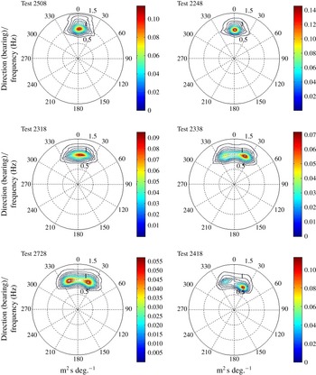
Measured directional spectra for several cases at position 7 (pentagon wave gauge array). All calculated using the IMLM.

The directional analysis (figure 2) shows that there is a slight directional offset for all tests of around
 $2^{\circ }$
caused by a small misalignment of the pentagon array relative to the wave maker. Tests with a crossing angle less than
 $20^{\circ }$
show as a unimodal spectrum with directional spread mainly dependent on crossing angle – effectively the two components appear to merge into one component with a wider directional spread. Tests with wider crossing angles show two clear directional components with features largely consistent with the requested direction and frequency. Similar features were observed at positions 1 and 5, but the two-component spectra with similar peak frequencies are not so well resolved using the IMLM at the three gauge arrays, so these are not shown.
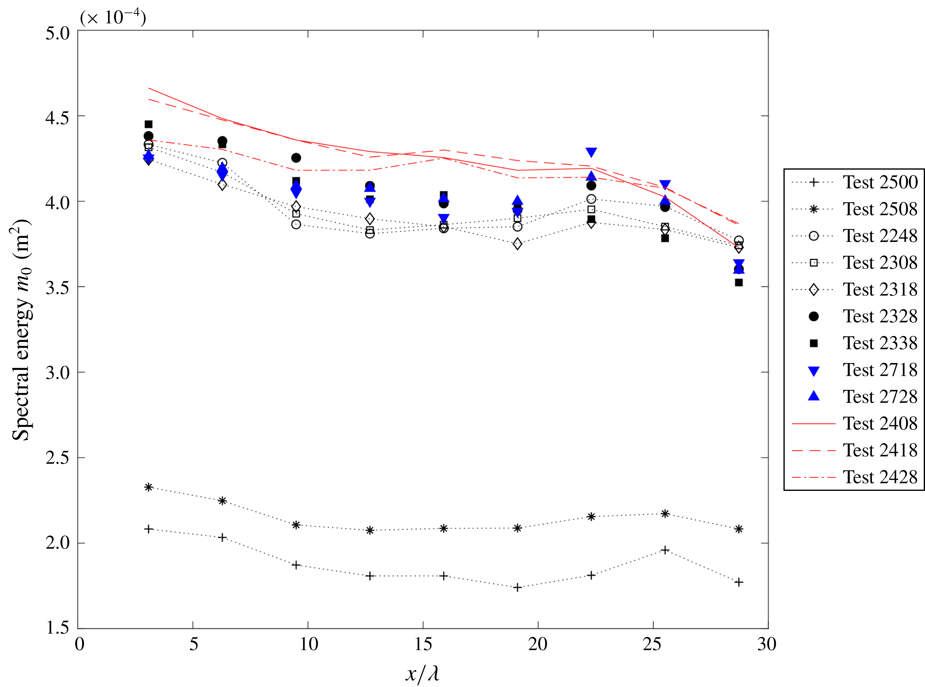
Change of spectral energy with non-dimensional distance down the centre of the tank for all test cases.

Plotting the zeroth-order moment of the variance density spectrum
 $m_{0}$
down the tank (figure 3) gives an indication of the total energy loss at the centre of the tank. The spectral energy
 $m_{0}$
drops off down the tank as is consistent with some form of energy dissipation. The rate of drop-off is not steady (indeed at some locations there is a slight increase) but there is some consistency between tests. A small number of breaking wave crests were observed in all bi-modal tests, but there was almost none in the unidirectional test (2500) which shows similar energy dissipation, so wave breaking is unlikely to be significant. The primary cause of the energy loss is almost certainly diffraction. The multi-flap wave maker does not cover the entire side of the tank and so energy loss to the edges must occur. One edge contains a wave absorber which will prevent most reflections, while on the other edge the end wave paddles were intentionally turned off to reduce reflections. There is also a wave absorber at the far end of the tank and reflections from this are likely to account for the small increases in energy seen at some locations near the end of the tank.
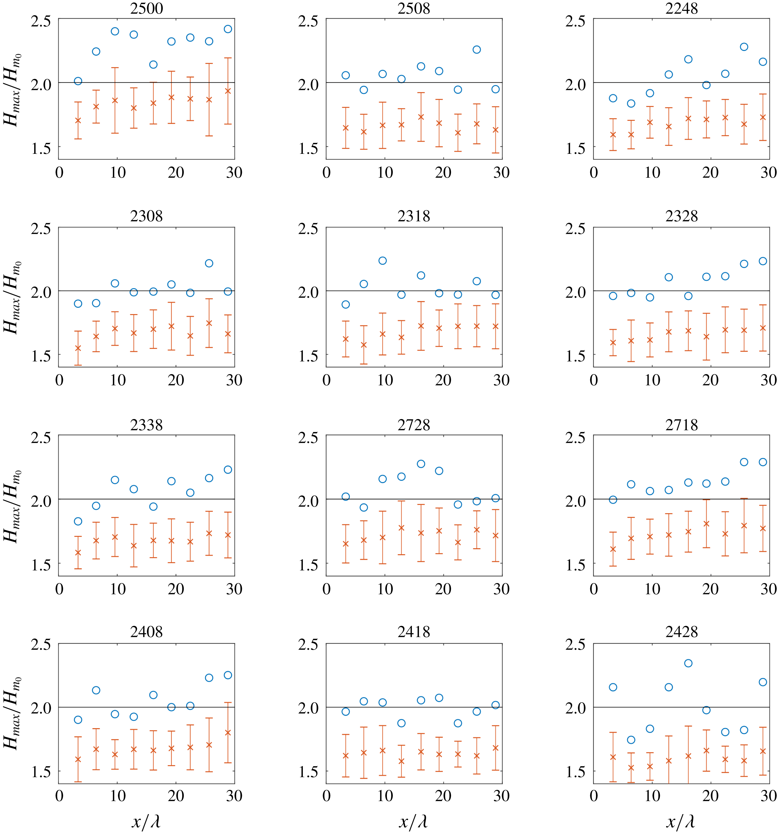
Evolution of
 $H_{max}/H_{m_{0}}$
down the basin for all tests. Circles show
 $H_{max}/H_{m_{0}}$
for the whole time series. The crosses are the mean value of
 $H_{max}/H_{m_{0}}$
over all segments when the time series is split into segments of 200 waves. The error bars represent the standard deviation from the mean over all segments. The line is at
 $H_{max}/H_{m_{0}}=2.0$
.

Figure 4 shows the evolution of
 $H_{max}/H_{m_{0}}$
down the designated centre of the tank, for the 12 selected test cases (for all cases the peak wavelength
 $\unicode[STIX]{x1D706}_{p}=1.56~\text{m}$
). Also shown are the mean and standard deviation of
 $H_{max}/H_{m_{0}}$
for each segment when the time series are split into segments of 200 waves. In the field, wave measurements are often taken for around 20 min every few hours, so with a peak period of 6 s, 20 min of data would be roughly 200 waves. The unidirectional case shows generally the highest values of
 $H_{max}/H_{m_{0}}$
, despite being the shortest test by a factor of 4. High maximum wave heights are observed for all tests (
 $H_{max}/H_{m_{0}}>2$
), but the maximum wave height gives no indication of the probability of occurrence. The mean maximum wave height for the 200 wave segments generally increases down the tank. The mean is highest for the unidirectional case 2500, and of the directionally spread test cases, case 2718 with two narrow components (
 $N=840$
and 200) crossing at
 $40^{\circ }$
shows the highest mean
 $H_{max}/H_{m_{0}}$
.
3.1 Exceedance probabilities
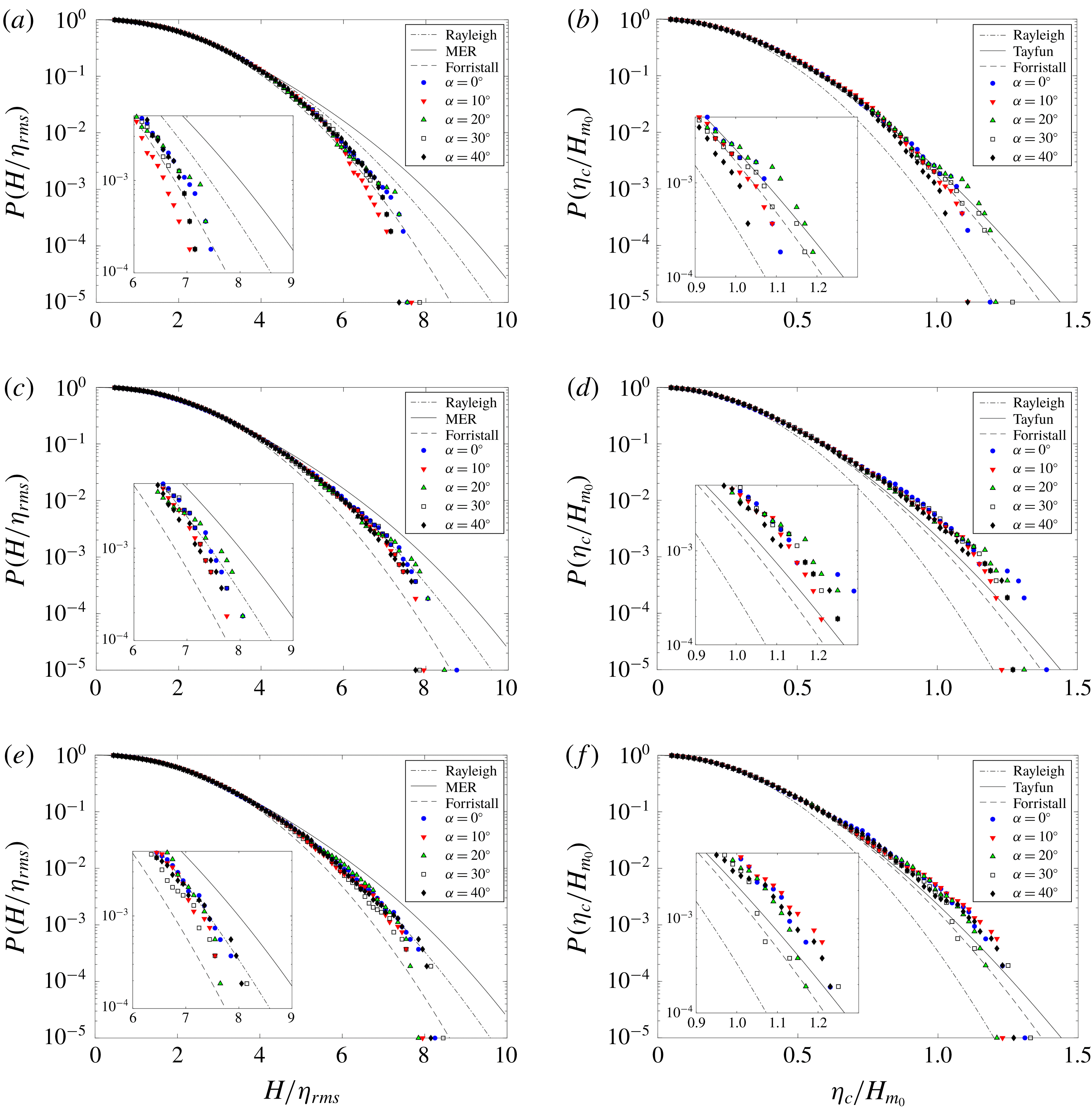
Exceedance probability distributions at different crossing angles for wave height
 $H/\unicode[STIX]{x1D702}_{rms}$
(a,c,e) and crest height
 $\unicode[STIX]{x1D702}_{c}/H_{m_{0}}$
(b,d,f) at position 1 (
 $x/\unicode[STIX]{x1D706}_{p}=3.2$
) (a,b), position 5 (
 $x/\unicode[STIX]{x1D706}_{p}=16.1$
) (c,d) and position 7 (
 $x/\unicode[STIX]{x1D706}_{p}=22.4$
) (e,f). Shapes show the experimental data. For (a,c,e) (wave height), the dotted line shows the Rayleigh distribution (2.3), the solid line shows the MER distribution (2.5) and the dashed line shows the Forristall distribution (2.4). For (b,d,f) (crest height), the dotted line shows the Rayleigh distribution (2.10), the solid line shows the Tayfun distribution (2.11) and the dashed line shows the Forristall distribution (2.12).

Figure 5 shows the exceedance probabilities for wave heights and wave crests at positions 1, 5 and 7 – the results show the effect of changing the crossing angle between the two components, but constant directional spreading of
 $N=50/N=200$
(note that the
 $/$
symbol here is for separation to show the different properties of the two components not a fraction). Taking the results for the wave heights first: for figure 5(a,c,e) the experimental results are closest to the Forristall distribution at position 1, but by position 5 the results are much closer to the Rayleigh distribution and remain the same at position 7. For the wave crest heights in figure 5(b,d,f) the experimental results are around the Tayfun and Forristall distributions at position 1 but by positions 5 and 7 they are generally well above the Tayfun distribution with some variations between the crossing angles, but no clear trends.
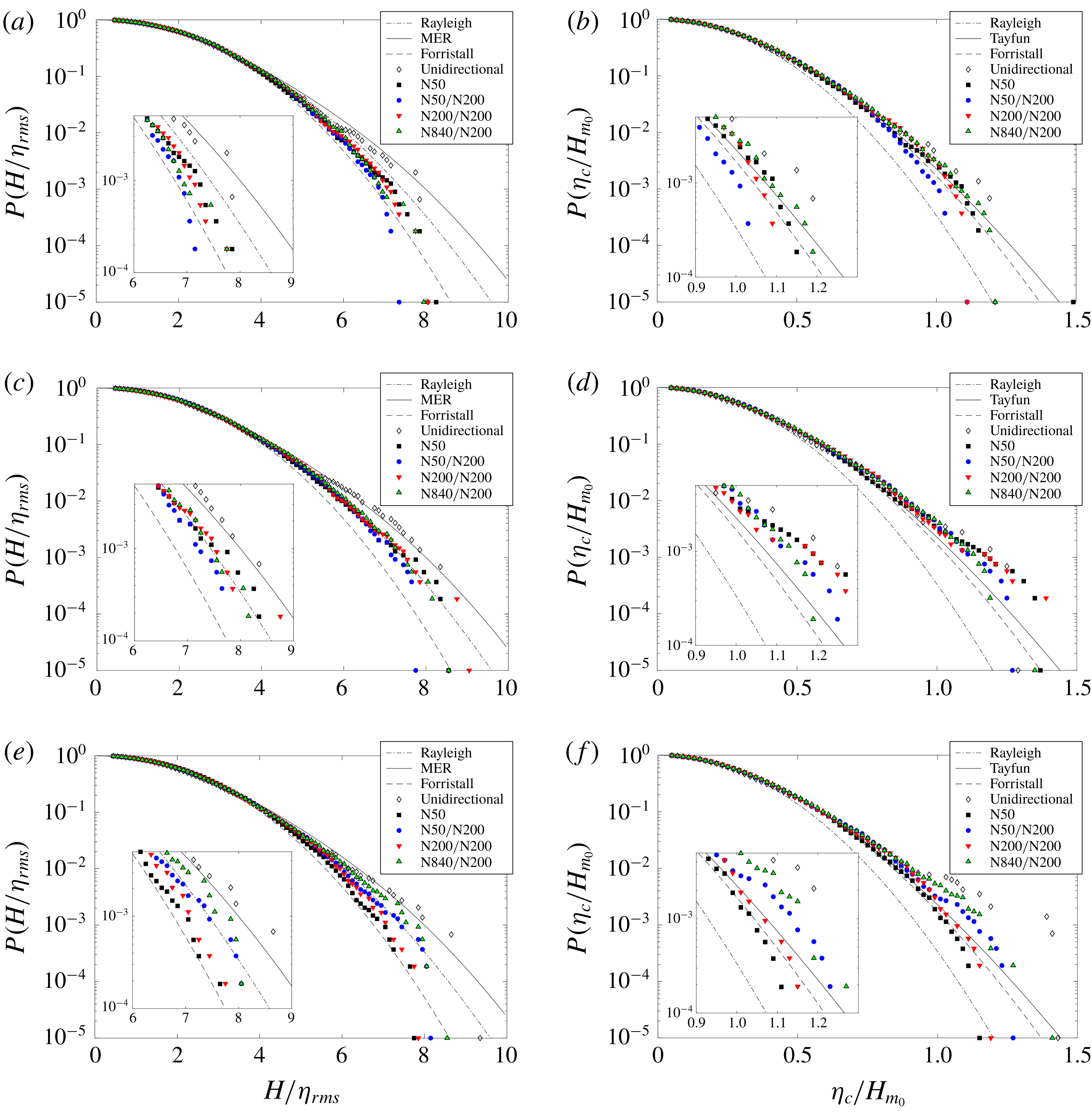
Exceedance probability distributions at different component directional spreads for wave height
 $H/\unicode[STIX]{x1D702}_{rms}$
(a,c,e) and crest height
 $\unicode[STIX]{x1D702}_{c}/H_{m_{0}}$
(b,d,f) at position 1 (
 $x/\unicode[STIX]{x1D706}_{p}=3.2$
) (a,b), position 5 (
 $x/\unicode[STIX]{x1D706}_{p}=16.1$
) (c,d) and position 7 (
 $x/\unicode[STIX]{x1D706}_{p}=22.4$
) (e,f). Shapes show the experimental data. Also shown are the unidirectional (test 2500) and single-component directionally spread (test 2508) cases. For (a,c,e) (wave height), the dotted line shows the Rayleigh distribution (2.3), the solid line shows the MER distribution (2.5) and the dashed line shows the Forristall distribution (2.4). For (b,d,f) (crest height), the dotted line shows the Rayleigh distribution (2.10), the solid line shows the Tayfun distribution (2.11) and the dashed line shows the Forristall distribution (2.12).

Figure 6 shows the exceedance probabilities for wave heights and wave crests at positions 1, 5 and 7 – the results show the effect of directional spread of the individual components with constant crossing angle. For the wave heights shown in figure 6(a,c,e) the experimental results are between the Forristall and Rayleigh distributions at position 1 and are close to the Rayleigh distribution by position 5. At position 7 the experimental results for a slightly narrower first component directional spreading (
 $N=200/N=200$
) are slightly below the Rayleigh distribution towards the Forristall distribution, while for a much narrower first component (
 $N=840/N=200$
) the experimental results are above the Rayleigh distribution towards the MER distribution. It is interesting to note that the case at
 $N=50/N=200$
is higher than that at
 $N=200/N=200$
but lower than that at
 $N=840/N=200$
. The unidirectional results are quite well described by the MER distribution at all positions and the results with a single directionally spread component are between the Forristall and Rayleigh distributions at position 1, close to the Rayleigh distribution at position 5 and close to the Forristall distribution by position 7.
The results for the wave crest heights shown in figure 6(b) show that the results with two narrow spectra are close to the Tayfun distribution at position 1, while the results with a broader component (
 $N=50/N=200$
) are between the Rayleigh and Forristall distributions at position 1. The unidirectional results are above the Tayfun distribution and the results with a single directionally spread component are quite well described by the Forristall distribution at position 1. By position 5 shown in figure 6(d) the experimental results are above the Tayfun distribution. At position 7 shown in figure 6(f), the test with the narrowest first component (
 $N=840/N=200$
) is the furthest above the Tayfun distribution, while the case at
 $N=200/N=200$
is on or just below the Tayfun distribution. Once again the case at
 $N=50/N=200$
is between the other two-component cases. The unidirectional results are well above the Tayfun distribution and the results with a single directionally spread component remain quite well described by the Forristall distribution at position 7.
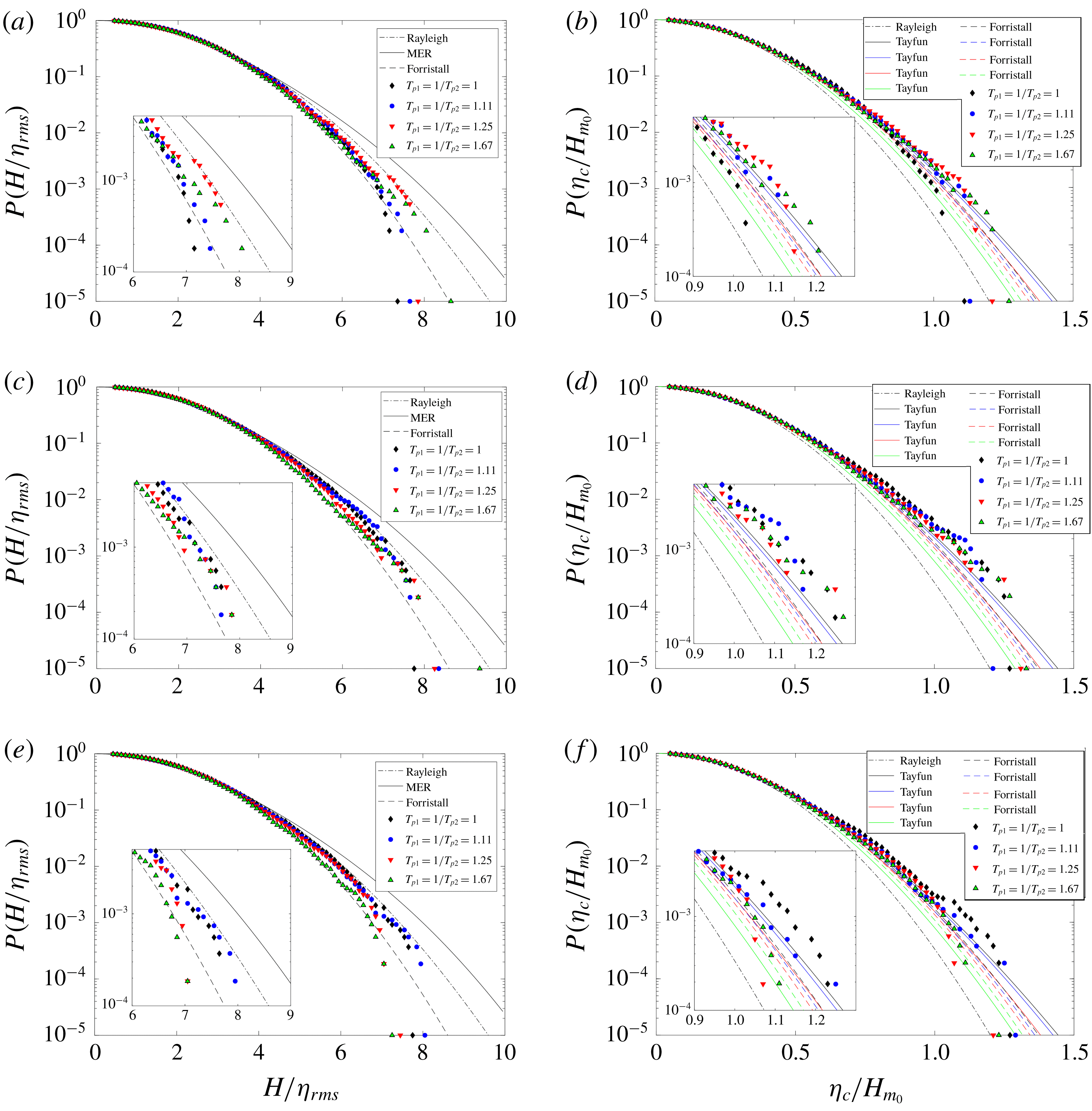
Exceedance probability distributions at different component peak frequencies for wave height
 $H/\unicode[STIX]{x1D702}_{rms}$
(a,c,e) and crest height
 $\unicode[STIX]{x1D702}_{c}/H_{m_{0}}$
(b,d,f) at position 1 (
 $x/\unicode[STIX]{x1D706}_{p}=3.2$
) (a,b), position 5 (
 $x/\unicode[STIX]{x1D706}_{p}=16.1$
) (c,d) and position 7 (
 $x/\unicode[STIX]{x1D706}_{p}=22.4$
) (e,f). Shapes show the experimental data. For (a,c,e) (wave height), the dotted line shows the Rayleigh distribution (2.3), the solid line shows the MER distribution (2.5) and the dashed line shows the Forristall distribution (2.4). For (b,d,f) (crest height), the dotted line shows the Rayleigh distribution (2.10), the solid lines show the Tayfun distribution (2.11) and the dashed lines show the Forristall distribution (2.12); the Tayfun and Forristall distributions are frequency dependent through
 $k_{p}$
and
 $S_{1}$
respectively so are coloured to indicate to which results they apply.

Figure 7 shows the exceedance probabilities for wave heights and wave crests at positions 1, 5 and 7 – the results show the effect of varying component peak frequency at a constant crossing angle of
 $40^{\circ }$
. For figure 7(a) the wave height results are between the Forristall and Rayleigh distributions at position 1. Further down the tank at positions 5 and 7, figure 7(c,e) shows the results are still slightly below the Rayleigh distribution towards the Forristall distribution except for the case at
 $T_{p_{1}}=1~\text{s}/T_{p_{2}}=1.67~\text{s}$
when the experimental results are clearly closer to the Forristall distribution.
For the crest heights at position 1 shown in figure 7(b), the experimental results are all close to the Tayfun distribution apart from the case at
 $T_{p_{1}}=1~\text{s}/T_{p_{2}}=1~\text{s}$
where the results are closer to the Forristall distribution. For figure 7(d,f) at positions 5 and 7 the experimental results are all above the Tayfun distribution, noting that for the case at
 $T_{p_{1}}=1~\text{s}/T_{p_{2}}=1.67~\text{s}$
the Forristall distribution is in fact above the Tayfun distribution, so in this case the experimental results are closest to the Forristall distribution.


Comparing the tails of the distributions between figures 5 and 6 shows clearly that changing the directional spreading of the individual components has more effect on the tails of the distributions than changing the crossing angles. Changing the crossing angles has relatively little clear effect on either the wave height distributions or the wave crest distributions, while changing the directional spreading of component 1 at a fixed crossing angle has quite a large effect. The kurtosis (shown in table 2) seems to correlate quite well with the above-noted features for figures 6 and 7 – the tests with higher overall mean kurtosis show higher exceedance probabilities. For the tests with different crossing angles in figure 5 the kurtosis varies from 3.133 to 3.255 but the exceedance distributions are all closely grouped.
Overall, for the experimental results for spectra that have developed down the tank (at position 7), the wave heights are reasonably well described by the Rayleigh distribution with the exception of the unidirectional case (long-crested) and the case with a single directionally spread component where the results are closer to the MER and Forristall distributions respectively. The results at position 7 for the wave crest heights are generally either slightly above or close to the second-order Tayfun distribution, again with the exception of the unidirectional (long-crested) results which are far above the Tayfun distribution and the single directionally spread component results which are well described by the Forristall distribution.
3.2 Kurtosis
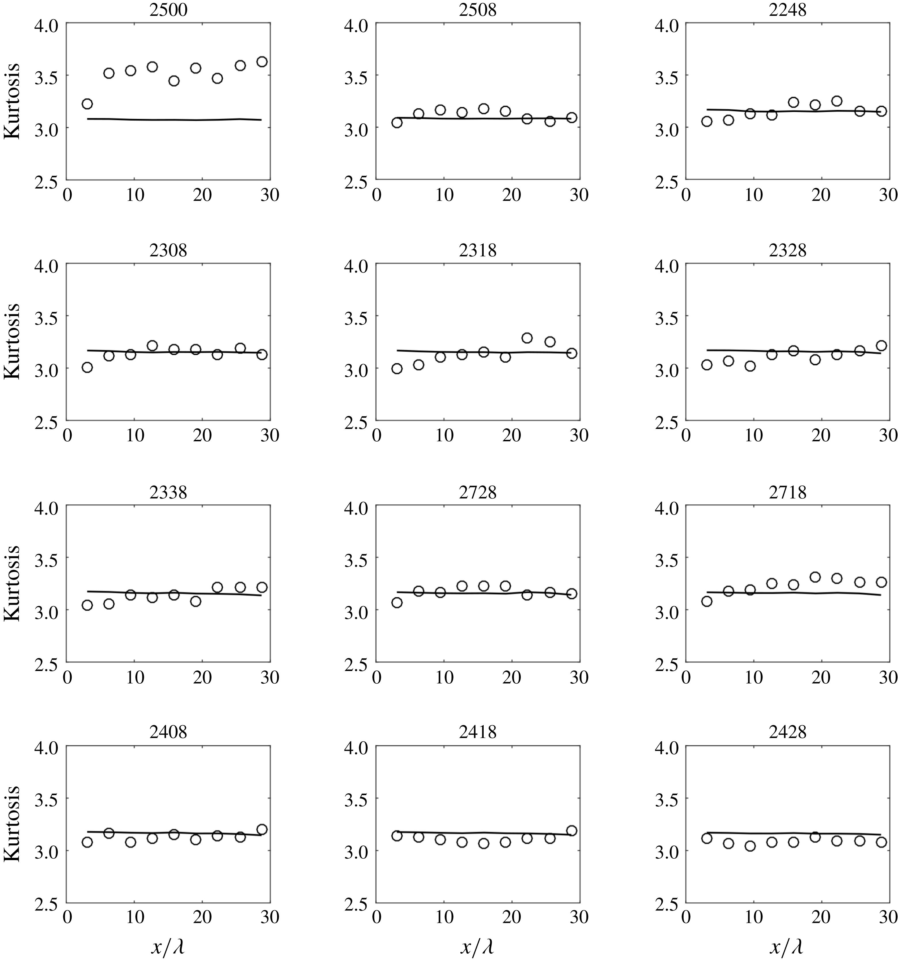
Evolution of kurtosis down the centre of the basin for all tests. The circles show the kurtosis
 $\unicode[STIX]{x1D707}_{4}$
(1.4) and the line shows a narrow-banded approximation of the second-order theoretical kurtosis distribution (1.5), both calculated from measured values at the centreline probes.

Previous studies have shown that increasing kurtosis is related to increasing rogue wave activity (Mori & Janssen Reference Mori and Janssen2006; Mori et al.
Reference Mori, Onorato and Janssen2011). Figure 8 shows the evolution of the kurtosis down the centre of the tank for the 12 selected test cases. The kurtosis is calculated from the whole combined file (80 min time series or 20 min for test 2500) for all kurtosis figures except for figure 10. For all the multi-directional cases, the kurtosis is considerably lower than the unidirectional case (test 2500). For all the multi-directional cases the kurtosis is close to the second-order theory and generally increases down the tank. There is no clear effect of changing the crossing angle between the two components for the angles tested. Using a narrower spreading factor for component 1 seems to increase the kurtosis to slightly above the second-order theory (test 2718 in particular). The conditions for cases 2718 and 2728 are more similar to the long-crested crossing seas used by Toffoli et al. (Reference Toffoli, Bitner-Gregersen, Osborne, Serio, Monbaliu and Onorato2011), who found increased kurtosis at around
 $40^{\circ }$
, and both cases show several points well above the second-order theoretical distribution. Note however that comparison between two crossing long-crested wave trains and crossing directional seas should be treated with caution. The measured excess kurtosis (
 $\unicode[STIX]{x1D707}_{4}-3$
) is up to 190 % of the second-order theoretical excess kurtosis for case 2718. The cases with a lower frequency for component 2 (tests 2408, 2418 and 2428) show slightly lower kurtosis than the cases with
 $T_{p}=1~\text{s}$
for both components.
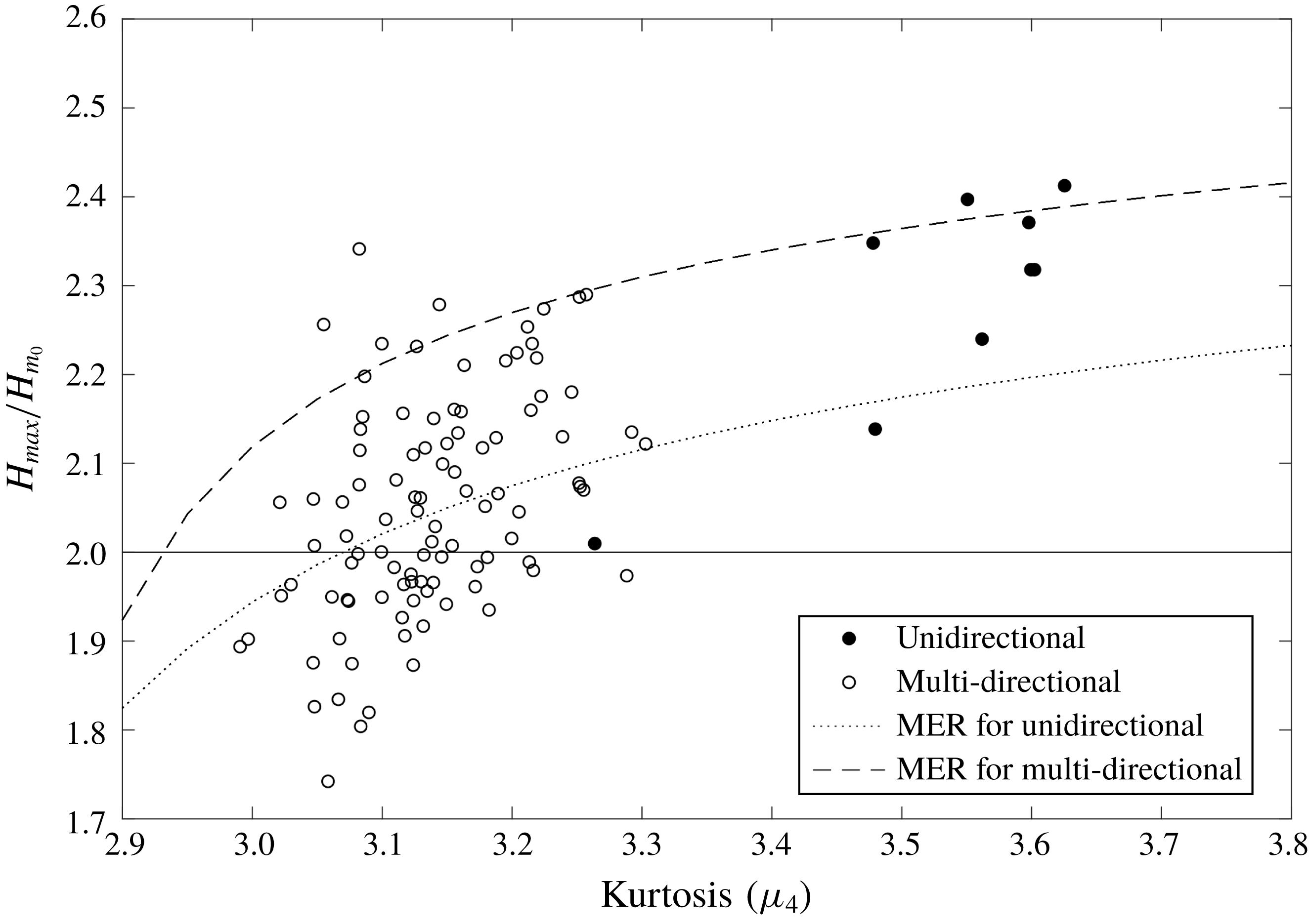
Plot of
 $H_{max}/H_{m_{0}}$
against kurtosis for all tests at nine positions down the tank. The unidirectional case (test 2500) is marked with filled circles. The lines show the theoretical relationship from integration of the MER probability density function (2.7) with 4800 waves for multi-directional cases and 1200 waves for the unidirectional case.

Figure 9 shows
 $H_{max}/H_{m_{0}}$
plotted against kurtosis for the same test cases and wave gauge positions presented in figure 8. Excepting the unidirectional case, the results are quite closely grouped with a mean kurtosis of around 3.14 and a mean
 $H_{max}/H_{m_{0}}$
of 2.05. The solid line shows the most commonly used definition of a rogue wave (
 $H_{max}/H_{m_{0}}>2$
). The results generally agree with the hypothesis that increasing kurtosis is related to increasing extreme wave activity as the trend is generally bottom left to top right across the figure (with some notable outliers). In addition to measured data, expected values calculated by numerical integration of the MER equation (2.7) are also given. Theoretical predictions of
 $H_{max}/H_{m_{0}}$
on the basis of number of waves and kurtosis
 $\unicode[STIX]{x1D707}_{4}$
are overestimated in comparison to the measured data. This agrees with the observation that the wave heights are quite well described by the Rayleigh distribution and hence below the MER distribution. The unidirectional results are grouped around the MER relationship as observed with the wave height exceedance plots.
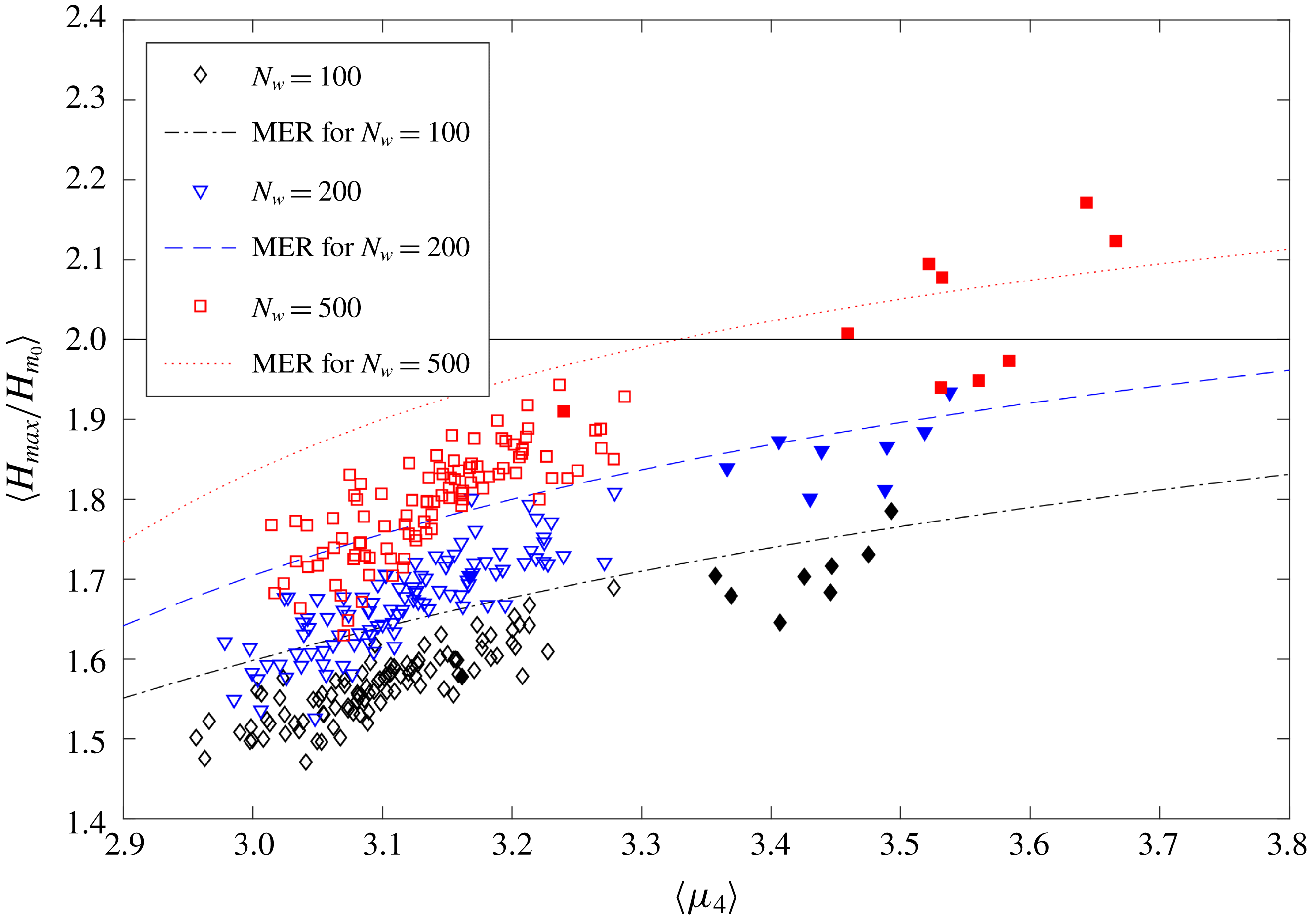
Averaged
 $H_{max}/H_{m_{0}}$
plotted against averaged kurtosis for all tests at nine positions down the tank, for three sample sizes. See associated text for a description of how these are calculated. The unidirectional case (test 2500) is marked with filled shapes. The lines show the theoretical relationship from integration of the MER probability density function (2.7) with the given number of waves.

Figure 10 shows the effect of sample size on the relationship between wave height and kurtosis. The surface elevation data were split into segments of 100, 200 and 500 waves and for each of these segments a value of
 $H_{max}/H_{m_{0}}$
and
 $\unicode[STIX]{x1D707}_{4}$
was calculated then averaged over the whole dataset at each of the nine locations down the tank. The averaged peak wave height ratio
 $\langle H_{max}/H_{m_{0}}\rangle$
increases with increasing averaged kurtosis
 $\langle \unicode[STIX]{x1D707}_{4}\rangle$
and with increasing sample size. The averaged peak wave height ratio is generally below the theoretical prediction except for the unidirectional case which is close to the model.
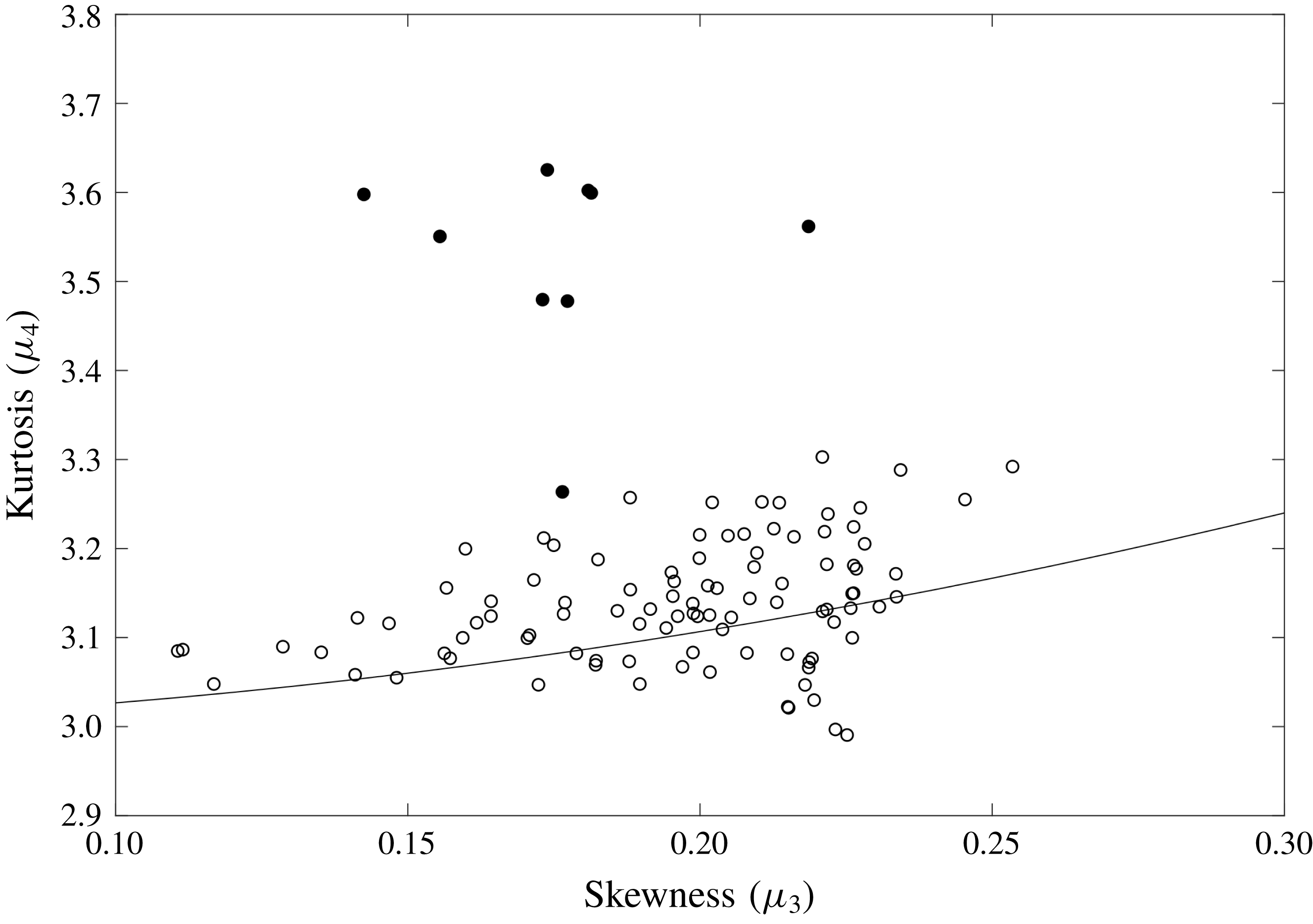
Kurtosis plotted against skewness for all tests. The unidirectional case (test 2500) is marked with filled circles. The line is the contribution to the kurtosis due to bound waves (3.1).

Figure 11 shows the kurtosis plotted against skewness, for the same test cases as above. With the exception of the unidirectional case, the values generally lie on or slightly above the theoretical second-order relationship describing the contribution to the kurtosis by bound waves represented by the solid line. The contribution to the kurtosis by bound waves is from
 $\unicode[STIX]{x1D707}_{4}=3+24(k_{p}\unicode[STIX]{x1D70E})^{2}$
and skewness
 $\unicode[STIX]{x1D707}_{3}=3k_{p}\unicode[STIX]{x1D70E}$
(Srokosz & Longuet-Higgins Reference Srokosz and Longuet-Higgins1986) giving
 $$\begin{eqnarray}\unicode[STIX]{x1D707}_{4}=3+{\textstyle \frac{8}{3}}\unicode[STIX]{x1D707}_{3}^{2}.\end{eqnarray}$$
Mori et al. (Reference Mori, Onorato and Janssen2011) present theoretical and empirical formulae for the relationship between directional spreading and kurtosis (
 $\unicode[STIX]{x1D707}_{4}$
). In the unidirectional case, a theoretical estimate of the kurtosis can be derived from the BFI (defined in (1.1))
 $$\begin{eqnarray}\unicode[STIX]{x1D707}_{4}=\frac{\unicode[STIX]{x03C0}}{\sqrt{3}}\text{BFI}^{2}+3.\end{eqnarray}$$
In the directionally spread case, an empirical estimate of the kurtosis can be derived from the empirical two-dimensional BFI (Mori et al. Reference Mori, Onorato and Janssen2011)
 $$\begin{eqnarray}\unicode[STIX]{x1D707}_{4}=\frac{\unicode[STIX]{x03C0}}{\sqrt{3}}\text{BFI}_{2D}^{2}+3,\end{eqnarray}$$
where
 $\text{BFI}_{2D}$
is given in (1.3). The two-dimensional BFI was not designed for bi-modal sea states and includes an empirical parameter specifically derived for unimodal short-crested waves. It is therefore of interest to test if the
 $\text{BFI}_{2D}$
can usefully be employed in bi-modal seas. There are several possible ways to define the degree of directional spreading
 $\unicode[STIX]{x1D70E}_{\unicode[STIX]{x1D703}}$
for a two-component directionally spread sea state and this is an area which would benefit from future study. The method used here is designed for unimodal multi-directional seas and calculates the overall mean directional spreading of the whole spectrum as described in § 2.1. Including the effects of bound waves gives (Mori & Janssen Reference Mori and Janssen2006)
 $$\begin{eqnarray}\unicode[STIX]{x1D707}_{4}=\frac{\unicode[STIX]{x03C0}}{\sqrt{3}}\text{BFI}_{2D}^{2}+24\unicode[STIX]{x1D700}^{2}+3.\end{eqnarray}$$
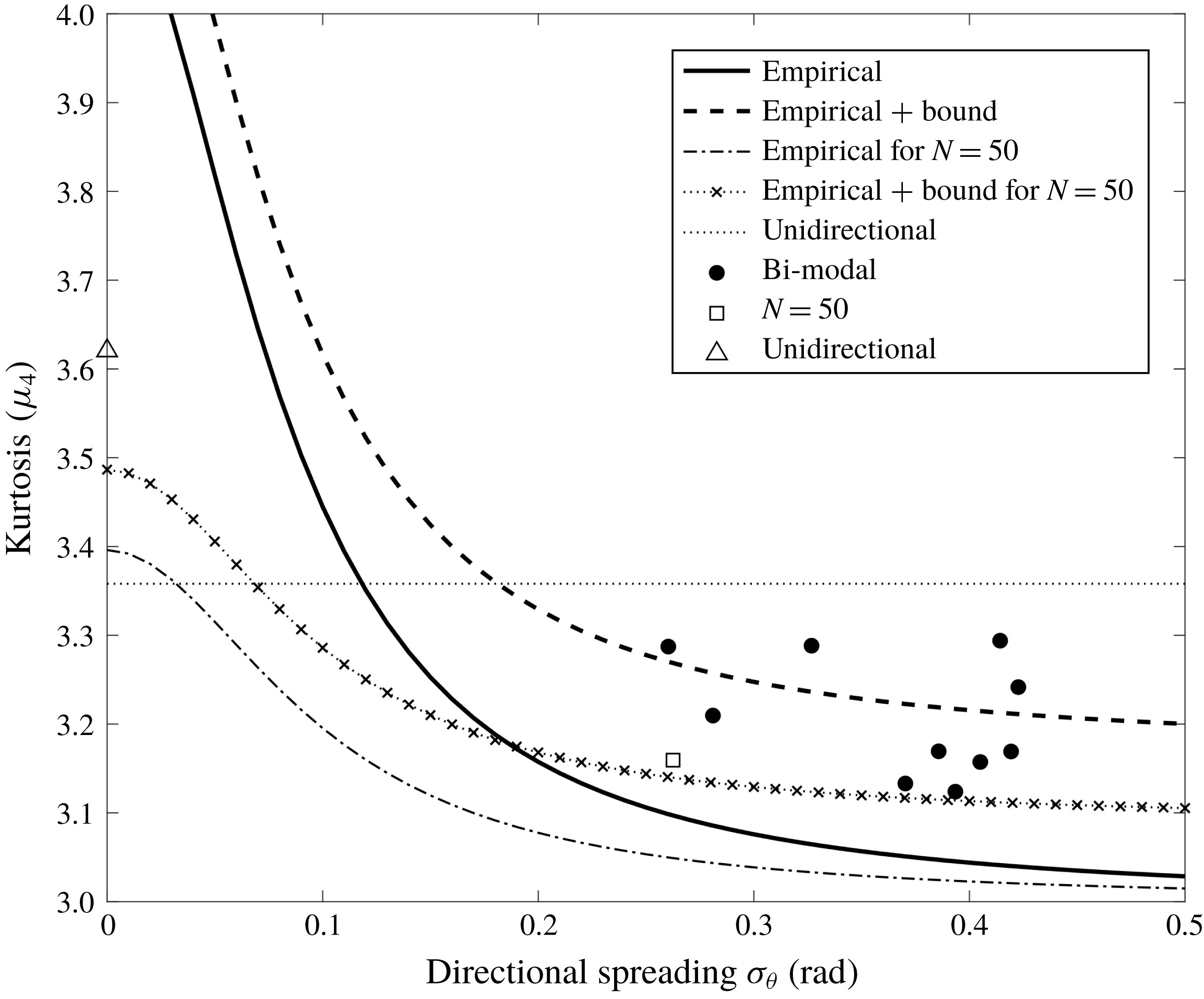
Figure 12 shows the three theoretical/empirical relationships as well as the experimental results for all test cases. The experimental kurtosis values are the maximum observed kurtosis at the pentagon wave gauge array and the spreading is calculated at the same position. The experimental results are distributed around the empirical relationship including bound mode effects, which agrees well with the conclusions of Mori et al. (Reference Mori, Onorato and Janssen2011), who found that for short-crested waves in the region
 $\unicode[STIX]{x1D70E}_{\unicode[STIX]{x1D703}}<0.2~\text{rad}$
the empirical solution including bound mode effects fitted the observed kurtosis well. The experimental value of kurtosis for the unidirectional case is well above the theoretical value.
Plot of maximum kurtosis down the tank against mean directional spreading
 $\unicode[STIX]{x1D70E}_{\unicode[STIX]{x1D703}}$
measured at position 7. Lines are for (3.3) (empirical), (3.4) (
 $\text{empirical}+\text{bound}$
) and (3.2) (unidirectional). The theoretical lines for
 $N=50$
are lower as
 $H_{m_{0}}$
is lower for the single-component cases.

4 Discussion
Rogue waves defined as
 $H/H_{s}>2$
(or
 $\unicode[STIX]{x1D702}_{c}/H_{s}>1.25$
) were detected in all tests. However, the probability of rogue waves is very small, of the order of 0.1 %–0.2 %, confirming that these events are rare in the sea states tested. Unlike studies with two unidirectional crossing components (Onorato, Proment & Toffoli Reference Onorato, Proment and Toffoli2010; Sabatino & Serio Reference Sabatino and Serio2015), the results here with two multi-directional crossing components do not show significantly different exceedance probabilities or kurtosis values for different crossing angles. Observing just the results with changing crossing angle, the wave height exceedance probabilities develop down the tank from a Forristall distribution at position 1 (
 $\unicode[STIX]{x1D706}/L=3.2$
) to a Rayleigh distribution at position 7 (
 $\unicode[STIX]{x1D706}/L=22.4$
). The crest height exceedance probabilities develop from a grouping around the Tayfun and Forristall distributions at position 1 to above the Tayfun distribution at position 7. For both wave heights and crest heights there is little difference among the crossing angles investigated. The kurtosis increases slightly down the tank to at or just above the second-order theoretical value, but in agreement with the exceedance probabilities there is no clear difference among the crossing angles.
In the case of the bi-modal crossing multi-directional waves investigated here, the directional dispersion of the spectrum poses a limit for the growth of kurtosis (Onorato, Osborne & Serio Reference Onorato, Osborne and Serio2002; Gramstad & Trulsen Reference Gramstad and Trulsen2007). The reduction of the quasi-resonant effects due to directionality is significant, resulting in only a slight increase in the kurtosis across the basin. For most of the multi-directional wave tests, the kurtosis value increases towards the middle of the basin but it does not significantly exceed the second-order prediction. A slight departure above the second-order estimation is only observed for two of the two-component test cases. Test 2318 with a crossing angle of
 $\unicode[STIX]{x1D6FC}=20^{\circ }$
showed an increase in the kurtosis towards the end of the basin reaching a value of 3.29 where the second-order theoretical value is 3.15. Test case 2718 with a directional spreading of
 $N=840/N=200$
and crossing angle of
 $40^{\circ }$
reached a slightly higher value of kurtosis at 3.30 against a second-order expectation of 3.17. This is also the only two-component test for which the wave height exceedance probability clearly exceeds the Rayleigh distribution at position 7 and the crest height exceedance probability is the furthest above the Tayfun distribution, implying that for these tests the directionality in the component spectra has more of an effect on rogue wave probability than the crossing angle.
The lowest values of kurtosis were recorded for the crossing sea states with different peak frequencies, which could be due to the basin being too short to allow for nonlinear interactions to take place when the peak frequencies are separated. Despite the unidirectional case having a lower wave steepness than the two-component cases, there is a clear departure in kurtosis values from the Gaussian statistics. This agrees quite well with the results of Onorato et al. (Reference Onorato2009) who found that for single-component directionally spread seas the wave heights were well described by the Rayleigh distribution and that for the wave crest heights the deviation above the Tayfun distribution reduced as the directionality in the wave field increased.
The
 $\text{BFI}_{2D}$
was formulated by Mori et al. (Reference Mori, Onorato and Janssen2011) using empirical data from unimodal directionally spread seas; here it is applied to bi-modal seas. Plotting kurtosis against directional spreading shows that the empirical formula with the bound modes effect included gives a reasonably good match to the data. Mori et al. (Reference Mori, Onorato and Janssen2011) found that for directional spreading
 ${>}0.2~\text{rad}$
, the bound mode effect contributes most to the kurtosis change, while the four-wave interactions are more significant with small directional spreading. For the two cases with the highest values of kurtosis (2718 and 2318), the empirical model slightly under-predicts the measured kurtosis even including the bound mode effects. The empirical relationships developed by Mori et al. (Reference Mori, Onorato and Janssen2011) give a reasonable approximation of the kurtosis of a crossing bi-modal directionally spread surface wave distribution when the directional spreading is calculated for the whole spectrum. The parametrisation by Mori et al. (Reference Mori, Onorato and Janssen2011) is based on the nonlinear Schrödinger equation to weak nonlinearity and narrow-banded spectra. Despite this, the results shown here clearly demonstrate a relationship between the kurtosis and the directional spreading, which is weakly affected by the crossing angle between sea-state components.
There are several limitations to this study. Only relatively steep wave conditions were studied and the values of directional spreading were below those typical of ocean wind waves. For the tests with two different peak frequencies it is likely that a longer basin would be needed to observe the full spectral development. Directional analysis at the far end of the tank showed that the requested input spectra were generally well reproduced in the tank, but differences between the measured and requested spectra noted were: a slight reduction in the crossing angle for the larger crossing angles and merging of the two components when the crossing angle was smaller. Reliably estimating the directional spreading of complex seas is difficult with point-measurement wave gauges even at the pentagon array. New measurement techniques need to be developed to capture the development across the whole basin, in particular the directional spectra need to be measured at multiple locations to improve the estimate of directional spreading.
Overall the results presented here indicate that the kurtosis and maximum wave height and crest height are more dependent on the component directional spreading than the crossing angle for crossing directionally spread seas. Bitner-Gregersen & Toffoli (Reference Bitner-Gregersen and Toffoli2014) on the basis of numerical studies emphasise the role of energy (steepness) and frequency in rogue wave probability and find that the maximum kurtosis occurs for
 $40^{\circ }$
independent of directional spreading. This suggests that further work is required to find when the kurtosis becomes less dependent on crossing angle and more dependent on directional spreading and to investigate the effect of steepness experimentally.
5 Conclusions
Laboratory experiments of two-component, directionally spread irregular waves were performed in one of the largest wave basins in the world. The effects of directional spreading, crossing angle and peak frequency on the development of the statistical properties of surface waves down the tank were investigated.
Overall, the directional spreading of the individual components appears to have more effect on the kurtosis and the exceedance probabilities than the crossing angle between the components. In particular, for one test condition with narrower directional spreading of both components the kurtosis and wave height exceedance probabilities were significantly increased compared to conditions with broader component directional spreading with the same crossing angle.
The kurtosis rarely exceeds the second-order theoretical value for the two-component crossing seas investigated here. The number of rogue waves in these experiments was relatively low, in agreement with previous experiments involving single-component directionally spread waves. The directionally spread test cases are found to be quite well grouped around a second-order correlation between kurtosis and skewness describing the effect of bound waves.
The wave height distribution is generally grouped around the Rayleigh distribution while the wave crest heights generally slightly exceed the second-order Tayfun distribution. For the test condition with narrower directional spreading of both components, the wave height distribution developed from well below the Rayleigh distribution at
 $x/\unicode[STIX]{x1D706}_{p}=3.2$
to close to the MER distribution at
 $x/\unicode[STIX]{x1D706}_{p}=22.4$
which was also the test and location with the highest kurtosis measured in all two-component tests. This suggests that linear and nonlinear processes take place down the tank and change the statistical wave properties. The MER distribution appears more appropriate for conditions with high kurtosis.
To our knowledge, we are the first to apply the empirical relationship between kurtosis and directional spreading derived by Mori et al. (Reference Mori, Onorato and Janssen2011) to two-component directionally spread crossing seas. The results showed that the kurtosis can be estimated reasonably well from the overall mean directional spreading using the empirical relationship including bound mode effects. This result opens the prospect of predicting the kurtosis from the directional spectrum, which can be then used in the estimation of the probability of extreme waves, but this will require further laboratory and field investigations.
Acknowledgements
The work described in this publication was supported by the European Community Seventh Framework Programme through a grant to the budget of the Integrating Activity HYDRALAB IV, contract no. 261520. This work was also partially supported by MEXT/JSPS KAKENHI grant no. 19H00782 in Japan and through the EPSRC SUPERGEN Wind Phase 2 (reference EP/H018662/1) programme in the UK. We would like to thank the staff of the Marintek facility Dr C. Pakodzi, Dr C. Trygve Stansberg and Dr I. Nygaard and also Dr V. Efimov from the Institute of Solid State Physics RAS, Chernogolovka, for important contributions to the experiments and for useful discussions.