1. Introduction

During winter, sea-ice deformation, including horizontal opening, closing and shearing, occurs at leads and ridges. These are linear features, tens of kilometers long, which can organize into lead systems (linear kinematic features (LKFs)) that run hundreds of kilometers across the Arctic (Reference Schulson and HiblerSchulson and Hibler, 1991; Reference KwokKwok, 2003). the ice pack is highly fractured. In synthetic aperture radar analysis (Reference KwokKwok, 2003) it is observed to undergo continuous deformation at 10 km scales, and the most energetic deformation is confined to narrow LKFs, and is an order of magnitude larger than the deformation outside LKFs. the spacing between leads varies depending on the confining stress on the ice pack and icepack strength (Reference Hutchings, Heil and HiblerHutchings and others, 2005), and also displays multiple scales of organization. Reference Overland, Walter, Curtin and TuretOverland and others (1995) demonstrate that the ice pack in the Beaufort Sea has ~10 km spacing between leads, and LKF spacing can be considered to be an order of magnitude larger. It can be argued that this behaviour either demonstrates an inherent scaling law for sea-ice deformation (such as discussed by Reference Schulson and HiblerSchulson and Hibler, 1991; Reference Weiss and MarsanWeiss and Marsan, 2004), or demonstrates differing mechanisms controlling ice dynamics at large and small scales (Reference Overland, Walter, Curtin and TuretOverland and others, 1995; Reference McNutt and OverlandMcNutt and Overland, 2003).

Analysis of strain-rate products from RADARSAT analyses and ice-drifting buoys by the team of Marsan, Weiss, Rampal, Stern and Lindsay (Reference Marsan, Stern, Lindsay and WeissMarsan and others, 2004; Reference Rampal, Weiss, Lindsay and SternRampal and others, 2008; Reference Stern and LindsayStern and Lindsay, 2009) demonstrates that sea-ice deformation is a fractal process in space and time. Reference Marsan, Stern, Lindsay and WeissMarsan and others (2004) identify that sea-ice deformation is localized, as deformation is concentrated at linear features. These results follow observations that leads and floe sizes follow a fractal distribution, and suggest that the mechanism controlling sea-ice failure is scale-invariant. the results, however, do not demonstrate why Reference Overland, Walter, Curtin and TuretOverland and others (1995) identified a hierarchy in the organization of leads in the Beaufort Sea. Determining the correct distribution for sea-ice deformation (active leads and ridges) is critical for quantifying surface heat fluxes and new ice formation (Reference Geiger and DrinkwaterGeiger and Drinkwater, 2005).

In this paper, we reproduce the Reference Marsan, Stern, Lindsay and WeissMarsan and others (2004) and Reference Rampal, Weiss, Lindsay and SternRampal and others (2008) results with an array of ice-drifting buoys that was designed to measure sea-ice deformation over cascading scales and relate the observed scaling relationships to changing weather. This unique, nested buoy array operated from late winter until early summer 2007.We investigate how deformation of the ice pack within the buoy array varies over length scales from 10 to 140km and timescales of hours to days. the impact of ice-drift sampling resolution, in space and time, on estimates of first-year ice growth is investigated. This applies the results of Marsan, Weiss, Rampal, Stern and Lindsay to test a deformation monitoring capturing sea-ice properties such as ice growth and open-water fraction. Recommendations for the design of sea-ice deformation monitoring systems are provided. We investigate if pack-ice deformation has a decorrelation length scale, and show how changing weather patterns impact the distances over which coherent deformation is experienced. Wavelet cross-coherence analysis of divergence on two spatial scales within the same region provides insight into emergent patterns in ice deformation. This sheds light on why leads appear to be organized on >100km scales. Our findings are summarized with suggestions on how to improve modelling and observation of sea-ice deformation.

2. Field Campaign

The Sea Ice Experiment: Dynamic Nature of the Arctic (SEDNA) field campaign utilized the Applied Physics Laboratory Ice Station (APLIS) in the Beaufort Sea in spring 2007. Two arrays of GPS ice drifters were deployed on 24 March in nested hexagons, of width 20 and 140 km, around APLIS (Fig. 1). All 12 buoys drifted with the ice pack and transmitted data until 22 June. These arrays formed the backbone of SEDNA (described in detail by Reference HutchingsHutchings and others, 2008; Reference HutchingsHutchings, 2009).

Fig. 1.

Map of GPS buoy positions on 25 March at 00:00Z. Buoy arrays are outlined in colour, referring to the spatial scale set to which the array belongs. the largest array, 140km scale, is outlined in black. Six 70 km scale arrays are red. There is one green 20 km scale array and four blue 10km scale arrays. the camp location is marked with a black square.

The GPS buoy positions are used to calculate strain-rate components, divergence and maximum shear rates (Fig. 2) of the ice pack within the array. the method we use, and error analysis, is outlined by Reference HutchingsHutchings and Hibler (2008). the SEDNA GPS buoys had a position error less than 10 m. Propagation of error analysis throughout strain-rate calculations indicates that strain-rate error is an inverse function of area enclosed by the buoy array and ice velocity. Errors are largest for small arrays moving slowly, and the signal-to-noise ratio becomes unacceptably small for arrays smaller than 3 km² moving at <0.002ms^–1. We flag, and do not include in our analysis, estimated strain rates that do not meet these two requirements, and estimate our strain-rate error as <1×10^–8 s^–1. the two arrays provide time series of ice-pack divergence and shear over four spatial scales that vary between 10 and 140 km. This is a unique dataset with which we can investigate the spatial scales of sea-ice deformation coherency. It is also useful for identifying if there is a scaling relationship linking the statistical properties of sea-ice deformation and the scale over which the deformation is observed.

Fig. 2.

Time series of (a) divergence rate, ε _I, and (b) maximum shear rate, ε _II, for the 140km scale array (black) and 20 km scale array (green). Total deformation rate is calculated as

As buoys provide time series of sea-ice deformation we can investigate the temporal evolution of the coherence of the ice-pack deformation, over different scales, during the spring transition from a relatively strong, connected, concentrated ice pack to a disconnected summer pack. As the data were collected in late winter and spring, we cannot resolve the full seasonal variability in scaling properties of sea-ice deformation, which has been identified by Reference Rampal, Weiss, Lindsay and SternRampal and others (2008) and Reference Stern and LindsayStern and Lindsay (2009). However, our analysis does provide independent verification of the deformation scaling properties of a compact ice pack, previously identified by Reference Marsan, Stern, Lindsay and WeissMarsan and others (2004).

The SEDNA deformation dataset has some features that are perhaps unusual and should be taken into consideration in following our analysis. At the start of the SEDNA campaign, a lead system opened in the 10km region around the ice camp. These leads were visually observed to be up to 1 km wide at times, and froze into areas of thin level ice (<50cm thick by mid-April) that subsequently ridged. We estimate that all level ice that grew in the inner buoy array during the SEDNA experiment was ridged by mid-June. This is not the case in the larger array, which sampled several lead systems including the system that ran through the inner array. This event was unusual in that we were able to sample the impact of a single, relatively large, deformation event on the ice pack over a range of spatial scales using drifting buoys.

3. Spatial Scaling of Strain Rate

SEDNA included nested buoy arrays (Fig. 1) that resolve icepack strain rate over a set of four spatial scales. For each buoy array we estimate strain-rate components and total deformation rate as described by Reference HutchingsHutchings and Hibler (2008). the time series of total deformation are plotted as a function of the square root of array area (length) in Figure 3. Data are clustered into sets of different length scales: around 10km (blue), 20 km (green), 70 km (red) and 140km (black). For each length scale set, we calculated the statistical moments of the distribution of total deformation. In Figure 3 a least-squares fit to the means of each length scale set is shown. Mean deformation rate, D, scales logarithmically

Fig. 3.

All realizations of deformation rate and length scale (square root of area), for each sub-array in all sets, are plotted in the colours defined in Figure 1. Mean sub-array length scale and mean deformation is plotted (black stars) for each buoy sub-array set defined in Figure 1. the least-squares fit to these values is shown as a solid line. the variance of deformation for each sub-array is plotted (black crosses), and the dashed line is least-squares fit to these points.

with length scale, L, such that

(1)

where H = -0:19. Reference Marsan, Stern, Lindsay and WeissMarsan and others (2004) found a similar relationship with an exponent of H = -0:2, for ice that covered the western Arctic during winter. Our result is an independent verification of the Reference Marsan, Stern, Lindsay and WeissMarsan and others (2004) results. It can be argued these results show that the fractal nature of sea-ice deformation is experienced by a region of ice as it evolves in time, as well as having a similar fractal distribution in space (Reference Marsan, Stern, Lindsay and WeissMarsan and others, 2004). We also find that other statistical moments of deformation (standard deviation, skewness and kurtosis) show scaling properties, increasing as the spatial scale decreases. Like Reference Marsan, Stern, Lindsay and WeissMarsan and others (2004), we find that sea-ice deformation displays multi-fractal properties (Fig. 4).

Fig. 4.

Moments, q, between 0.5 and 4, of deformation rate, ( D^q ), plotted against length scale. the colour of the mean value, plotted as crosses, corresponds to buoy array shown in Figure 1.

Our analysis supports the hypothesis of Reference Marsan, Stern, Lindsay and WeissMarsan and others (2004) that sea-ice strain rate is localized. Like Reference Marsan, Stern, Lindsay and WeissMarsan and others (2004), we find that as spatial scale decreases, larger strain rates become apparent, indicating the largest strain rates are accommodated by a small portion of the buoy array area. Another signature of this localization is that the variance of sea-ice deformation increases as spatial scale reduces, which we find in agreement with Reference Marsan, Stern, Lindsay and WeissMarsan and others (2004). Reference Stern and LindsayStern and Lindsay (2009) found that this localization is a property of the spatial structure of the deformation field.

4. Temporal Scaling

For each buoy position time series, we can subsample the time series, to calculate deformation time series with varying temporal resolution. the highest resolution available is 10 min. the lowest resolution we subsample at is 10 days. This provides three orders of magnitude in temporal resolution for which we can search for the existence of a temporal scaling relationship. Similar scaling relationships (Fig. 5) are found for all sub-arrays, which have spatial scales varying from 6 to 140 km.

Fig. 5.

Least-square fit to the means of deformation rate at each timescale sampled for all SEDNA sub-arrays. the colour corresponds to the spatial scale family the sub-array belongs to: 10 km (blue), 20 km (green), 70 km (red) and 140 km (black). the gradients of the smallest arrays are close to –1.

The first observation we can make from Figure 5 is that there is a log–log linear scaling relationship between deformation and timescale, T, where D ∝ 1/T, such that the evolution of deformation in time can be thought of as a pink noise process. Sea-ice deformation at spatial scales between 6 and 140 km displays non-equilibrium critical behaviour. This is an important observation for those wishing to model sea-ice deformation.

At the highest and lowest resolutions the scaling behaviour falls away from linear. This is more apparent in section 4.1, but we comment on this here as it does affect our interpretation of the data. At high temporal resolutions, from 10 min to <1 hour, the GPS position error propagated through our calculations becomes similar in magnitude to the size of the deformation, so at these higher resolutions the scaling relationship represents GPS noise. There is a lower timescale limit over which deformation can be reliably calculated with GPS, and this limit varies from 30 min to 1 hour across the spatial scales resolved in SEDNA. Smaller spatial scales have a larger lower temporal sampling limit.

For the lower temporal resolutions, above daily sampling, we find the scatter in mean deformation displays large variability. the gradient of the scaling relationship appears to increase, becoming more of a red-noise process, and for some sub-arrays the magnitude of deformation increases. This excursion from the scaling relationship experienced at timescales between 1 hour and 1 day appears small (<10% of mean deformation rate). However, in section 4.1 it is demonstrated that these small deviations have a dramatic impact on estimation of ice growth in leads.

Spectra of total deformation rate, for sub-arrays of varying spatial scale, are plotted in Figure 6. These spectra indicate, like Figure 5, that deformation is a pink noise process. Unlike Figure 5, Figure 6 encompasses all information about the deformation statistical distribution (Figure 5 only provides information about the statistical mean). Comparison of Figures 5 and 6 suggests that the quantity investigated in Figure 5, mean deformation, does not represent the full scaling behaviour of sea-ice deformation time series (sea-ice deformation has a non-Gaussian distribution, with statistical moments that vary with space- and timescales). This suggests that spectral analysis techniques may be more appropriate for investigating the scaling properties of sea-ice deformation than simply considering the scaling properties of the mean.

Fig. 6.

Spectral density of deformation, estimated with a fast Fourier transform method (Jenkins and Watts, 1969). Spectra are calculated from each sub-array, and mean log–log linear fit to spectra with spatial scales of 10 km (blue), 20 km (green), 70 km (red) and 140 km (black) are plotted. At the largest spatial scale, 140 km, the spectra can be approximated by red noise. the other spectra are pink, becoming whiter as spatial scale decreases. At the largest spatial scale, 140 km, the spectra have a slope of –2, and this slope decreases with reducing spatial scale: –1.8 (70 km), –1.4 (20 km) and –1.3 (10 km).

The degree of whitening of the spectra increases as length scale reduces. There is no apparent universal scaling parameter for sea-ice deformation that applies across spatial scales from 10 to 70 km. To understand this, we need to consider the following point: if ice rheology is not significant in the force balance on the ice pack, we expect sea-ice velocity and deformation time series to follow atmospheric and oceanic forcing on the ice pack. Hence we would expect the time series of deformation to possess red spectral character. Ice interaction acts to dissipate energy, whitening the spectra of deformation. This suggests we are seeing the greatest energy dissipation at the smallest length scales, which resolve only one or two leads. As length increases, more lead systems are encompassed in the buoy array. We know that these lead systems develop in patterns that are, to first order, determined by the wind forcing on the entire Beaufort Sea ice pack (Reference Walter and OverlandWalter and Overland, 1993) or at least to the 1000 km (synoptic) scale of atmospheric synoptic systems (Reference Geiger, Zhao and LiuGeiger and others, 2000); and that these lead patterns have fractal characteristics (Reference Weiss and MarsanWeiss and Marsan, 2004). It follows that if we sample the ice-pack deformation below the synoptic spatial scale, ice deformation might show self-organized critical behaviour (as shown in Fig. 5 and 6) and that organization increases as the length scale increases and lead patterns, associated with particular storms, become apparent. Figure 6 indicates that organization of the sea-ice deformation field reflects atmospheric variability over length scales of 140 km. At smaller resolutions, there is an increasing randomness in the deformation field sampled, and our results suggest that individual lead deformation may be close to white noise.

4.1. Impact of spatio-temporal resolution on mass-balance estimates

The buoy array area or divergence time series can be used to estimate new ice growth in leads and redistribution of this new ice to ridges. To do this we use a model of thermodynamic ice growth and redistribution that is driven by the observed buoy array divergence. This model uses climatological ice-growth/-melt rates from Reference Maykut and UntersteinerMaykut and Untersteiner (1971) and the assumption that thinnest ice is ridged preferentially. Figure 7 shows a time series of new level ice and ridged ice volume estimated for the large 140 km scale array, with hourly temporal resolution.

Fig. 7.

Divergence of the largest SEDNA array, between 26 March and 22 June (a), is used to calculate open-water fraction (b) and ridged ice area. A model of ice growth, using Reference Maykut and UntersteinerMaykut and Untersteiner (1971) growth rates, tracks the thickness of ice grown in leads, in 20 0.5 m thickness categories. on closing, thin ice is ridge preferentially, and subsequently tracked as ridged ice thickness. Time series of modelled level ice volume (c) and ridged ice volume (d) are shown, and the sum of these (the total volume of new ice) is shown (e).

The localization and fractal character of ice-pack strain rate is a result of the ice-pack deformation occurring at leads and ridges. Divergence of arctic sea ice increases in mean magnitude and variance as the spatial scale of estimated divergence reduces. This means that measurements taken over smaller scales will result in larger estimates of lead opening and closing rates. It affects estimation of new ice growth. In Figure 8, we plot the area-averaged mean thickness of ice grown between 26 March and 22 June as a function of array length scale.

Fig. 8.

Area-averaged mean thickness of ice grown between 26 March and 22 June, as a function of array length scale (the square root of mean array area). Mean values for the 10 and 70 km arrays are plotted as stars. the least-squares fit has a gradient of –0.7 (m)/log (km).

Figure 8 indicates that our calculation of new ice growth has fractal properties, like lead area and divergence. the smaller the length scale over which divergence and growth is estimated, the larger the estimated new ice thickness. Clearly, large-scale deformation measurements underestimate the open-water fraction, closing rate and hence new ice growth. To prevent this problem, either individual leads must be resolved in the measured deformation field (requiring observations at better than 10km spatial scales), or some distribution of lead divergence, perhaps a fractal distribution, must be assumed over the region.

Temporal resolution also has an impact on ice growth calculations. In Figure 9 we show the relationship between new ice growth and time resolution for all SEDNA sub-arrays. Over the timescales which we have identified to be not affected by GPS noise and low-resolution sampling issues (1 hour to 1 day), we see a scaling relationship that is similar for all spatial scales.

Fig. 9.

Area-averaged mean thickness of ice grown between 26 March and 22 June 2007 (G), as a function of timescale (T) resolved. Mean values for all arrays are plotted as crosses. Each solid line is a least-square fit to the mean ice growth in each sub-array. These lines follow the relationship G ∝ T^β , β = 0:30 with standard deviation 0.03. the colours correspond to the spatial scale set to which the array belongs: 10 km (blue), 20 km (green), 70 km (red) and 140 km (black).

Sub-hourly resolutions introduce increasing errors into the deformation calculation, through GPS noise, so ice growth is not correctly estimated. Note that other measurement methods for ice position and deformation have larger errors than GPS (Advanced Research and Global Observation Satellite (ARGOS) position error is ~300m and the RADARSAT Geophysical Processing System position error is 320m (Lindsay and Stern, 2003)), so they cannot resolve sea-ice deformation below 3 hours (Hutchings and others, unpublished information). the calculation of new ice growth in leads, and scales that can be resolved, is impacted by the divergence measurement error such that measurements with lower accuracy have a large temporal sampling cut-off and will tend to overestimate ice growth.

At lower resolutions the changing ice growth rate due to thickening in the Reference Maykut and UntersteinerMaykut and Untersteiner (1971) model is insufficiently resolved, resulting in overestimation of ice thickness in an opening pack. Between hourly and daily resolutions, where our calculations are reliable, we see smaller ice growth rates at higher resolutions because the greater fluctuation in ice-pack divergence resolved at these scales retards ice growth. Figure 9 indicates the importance of resolving the temporal evolution of leads in sea-ice mass-balance estimation.

Basal ice growth during our experiment period was ~0.2 m. New ice growth varied between half and five times the basal growth rate, depending on the spatial and temporal scale over which new ice growth was estimated. This new ice is a significant part of the winter ice growth in the Beaufort Sea. Correct representation of it in models and accurate observations of new ice growth are important for correctly representing the sea-ice mass balance.

4.2. Are spatial and temporal scaling relations independent?

A natural question following from our separate investigation of spatial and temporal sampling is: ‘is the spatial scaling relationship robust to temporal sampling?’. We find that it is not, as did Reference Rampal, Weiss, Lindsay and SternRampal and others (2008) and Reference Geiger, Drinkwater, Dempsey and ShenGeiger and Drinkwater (2001). Figure 10 shows H, from Expression (1), estimated for deformation that has been calculated with different temporal resolutions. We find a trend where the magnitude of H decreases as timescale increases, as did Reference Rampal, Weiss, Lindsay and SternRampal and others (2008). This suggests a whitening of the spatial scaling character of sea-ice deformation as temporal resolution decreases, suggesting that greater random noise is introduced into the scaling estimate as the number of buoy positions used to calculate the deformation time series is reduced. Reference Geiger, Zhao and LiuGeiger and others (2000), Reference Geiger and DrinkwaterGeiger and Drinkwater (2005) and Reference Rampal, Weiss, Lindsay and SternRampal and others (2008) point out similar coupling between spatial and temporal scaling relations for sea-ice deformation across the Arctic, in both summer and winter. the observation that there is a relationship between temporal and spatial scaling means that we can relate measurements of sea-ice deformation over different scales, as has been done by Reference Geiger, Zhao and LiuGeiger and others (2000) and Reference Geiger and DrinkwaterGeiger and Drinkwater (2005) using a different approach to the one we take in section 4.3. It also means we can investigate the length scales over which ice-pack deformation is coherent given a time series of sea-ice deformation measured at a variety of spatial scales.

Fig. 10.

Gradients calculated as in Figure 3, for time sampling that varies between 10 min and 10 days. A least-square fit to values of H and log T is shown. the gradient of this fit is 0.5 (log day) and only varies by ±0.1 (log day) if the least-square fit is confined to less time-sampling spread.

4.3. Spatio-temporal scaling of coherence of divergence

Ice velocity and strain rate do not behave as stationary processes. Their statistical properties, including mean and standard deviation, evolve over synoptic and seasonal timescales. We also know that divergence between buoy arrays that are closely spaced, of magnitude 10 km, has correlation that exhibits large spatial variation, varying from weakly anticorrelated, to uncorrelated to strongly correlated over short distances, <70km (Hutchings and Roberts, in press). the degree to which the two hexagonal SEDNA buoy-array divergence time series are correlated varies by up to 50% depending on the time period over which the correlation analysis is performed. This suggests a classic decorrelation length scale is not appropriate for sea-ice deformation.

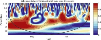
Figure 11 provides the wavelet cross-coherence between large (140 km) and small (20 km) scale divergence. This has been calculated following the methods of Reference Grinsted, Moore and JevrejevaGrinsted and others (2004) using a sixth-order derivative of Gaussian wavelet (DOG6) with 0.25 octaves per scale. This analysis reveals that there is significant coherence over synoptic weather-scale periods. There are specific features in Figure 11 that are insightful for understanding the changing coherence length scale for sea-ice deformation, and we discuss the four main points here.

Fig. 11.

The coherence between wavelet spectra of divergence time series for small (20 km), and large (140 km) buoy arrays. 95% significance levels are encircled by solid lines, and the cone of influence is shown with a bold solid line. 00:00Z on 1 May 1 and 1 June are indicated by their month.

1. 1. Significant power in both divergence and ice velocity is experienced for the semi-diurnal time period, driven by inertial motion of the ice and ocean. During late winter the magnitude of this semi-diurnal power is low (Hutchings and Roberts, unpublished information), but there are times when a semi-diurnal oscillation in divergence is present. During some of these times, there is coherence between divergence for small and large SEDNA arrays. Our main finding is that the times over which divergence is responding with a semi-diurnal period are sporadic and last for <2 days. This suggests that, in the Beaufort Sea in winter, inertial motion has a secondary impact on sea-ice deformation, and winds are more important in the force balance on the ice pack.

2. 2. Coherence in ice divergence is experienced across the 140 km SEDNA region over synoptic time periods (3–8 days), for the majority of the time series. There are, however, three times when divergence becomes incoherent: 30 April–2 May, 5–10 May and 10–15 June.

3. 3. During the first part of the time series, divergence is coherent across the 140 km SEDNA region for time periods longer than the synoptic timescale. This suggests a degree of connectivity of the ice pack, whereby ice is responding in a coherent fashion to longer-range forcing than local synoptic events. During the 16 day period during which coherence is experienced, several different weather systems impacted ice dynamics in the Beaufort Sea. We can infer the length scale of influence for storms impacting ice in this region during late winter is much larger than the scale of the actual storm.

4. 4. Around mid-May, coherence is lost over time periods longer than the synoptic period. This indicates a transition between winter and spring pack, with the connectivity of the pack reducing in spring. This transition occurs during one synoptic event, when the ice pack was observed to open. A high-pressure ridge system sat over the Beaufort Sea around 15 May, leading to a diverging ice pack, probably under clear skies. This was the first event, after the return of sunlight, that allowed substantial solar heating of the upper ocean through leads, and probably heralded the start of spring in the southern Beaufort Sea. It is interesting that after this single event, coherence was never regained over long time periods; connectivity of the ice pack had broken down during the high-pressure event, such that storms at a distance no longer impacted sea-ice deformation at the SEDNA site.

We find ice-pack divergence is coherent over synoptic timescales, over distances of 140 km. In winter, fortnightly coherence timescales are observed, suggesting a coherence length scale of order 1000 km. This large-scale coherence breaks down rapidly in spring during one synoptic event. Coherence is small over periods less than the synoptic timescale. We also see an increase in deformation variability and whitening of the deformation spectra at smaller scales less than 140 km. This indicates that the deformation of a smaller-scale, <140km scale region embedded in a larger region cannot be predicted from deformation observations at the larger scale.

In winter, a connected ice pack will be consolidated and allow transmission of internal ice stress over large (regional-scale) distances, leading to coherent behaviour of the icepack strain-rate components over these distances. We estimate that this coherence distance is of the order 1000 km during late winter, but coherence breaks down below the synoptic scale. After the transition (around 15 May) the coherent length scale is similar to the synoptic length scale in the atmosphere (hundreds of kilometres). However, there were times when the small buoy-array divergence was not coherent to the large array divergence over synoptic periods. Our analysis indicates the notion of a decorrelation length scale for ice-pack divergence does not explain all spatial variability in divergence fields. Divergence is incoherent and hence uncorrelated between temporal scales smaller than the atmospheric synoptic scale and between spatial scales less than 100 km, but displays coherence across larger scales.

5. Discussion and Concluding Remarks

In this paper, we produce findings in agreement with Reference Marsan, Stern, Lindsay and WeissMarsan and others (2004) and Reference Rampal, Weiss, Lindsay and SternRampal and others (2008) using a set of ice-drifting buoys that were deployed in an array, designed for investigating temporal and spatial scaling in sea-ice deformation. the array design allows deformation scaling behaviour, and changes in coherence of deformation events between large and small spatial scales, to be related to weather. We find similar scaling relationships to Reference Marsan, Stern, Lindsay and WeissMarsan and others (2004), Reference Rampal, Weiss, Lindsay and SternRampal and others (2008) and Reference Stern and LindsayStern and Lindsay (2009) with these data, and we identify the length-and timescales over which the error characteristics of our deformation analysis allow representation of the scaling relationship. We highlight that the multi-fractal nature (demonstrated by Reference Marsan, Stern, Lindsay and WeissMarsan and others, 2004) of deformation is important in characterizing its statistical properties. Time series of deformation is a pink-noise process, which indicates it is controlled by a balance between external forcing and internal dissipation. We suggest spectral and wavelet methods may be more appropriate for scaling analysis of sea-ice deformation, compared to the methods of Reference Marsan, Stern, Lindsay and WeissMarsan and others (2004), Reference Rampal, Weiss, Lindsay and SternRampal and others (2008) and Reference Stern and LindsayStern and Lindsay (2009), and find that dissipative processes become more apparent as the region over which divergence is estimated decreases.

We investigated how position measurement resolution (sampling interval in space and time) can impact estimates of ice growth over winter, and find that, to correctly simulate ice growth, deformation must be resolved at the lead scale with at least hourly time sampling. However, the fact that deformation scales with spatial and temporal sampling rate, in a well-behaved way, suggests the statistical properties of deformation at small scales can be modelled given larger-scale measurements. This would allow estimation of integral properties of the deformation field (e.g. end-of winter first-year ice thickness) to be improved.

It is intuitive that the scaling properties of deformation should be related to the coherence length scale experienced by the ice pack. Hutchings and others (unpublished information) found that the correlation in deformation time series between 10 km² areas of ice reduces in variance as the distance between ice areas increases. the data were collected in early summer, and suggested that deformation correlation was lost at distances greater than the synoptic scale. In our experiment, we use cross-wavelet coherence analysis to investigate how coherence length scale is related to weather. an opening ice pack, with predominately anticyclonic forcing, displays lower coherence length scale than a closing ice pack, under predominately cyclonic forcing. Classic decorrelation length-scale analysis is an inappropriate metric for sea-ice deformation. the randomness, or degree of whiteness, of deformation time series increases as spatial scale decreases. At sub-synoptic scales, deformation does not display coherence across regions of the ice pack. Coherence is apparent over synoptic scales and over longer periods when the ice pack is predominately closing.

Reference Rampal, Weiss, Lindsay and SternRampal and others (2008) show scaling properties of deformation are different in summer and winter. Reference Stern and LindsayStern and Lindsay (2009) find an annual cycle in the fractal dimension of deformation, and find differences between perennial and seasonal ice packs. These two papers led us to postulate that these changes in fractal dimension could be related to changes in coherence length scale of deformation. However, when we tested this assumption by performing our scaling analysis over two separate periods (before and after 15 May) we did not find significant changes in fractal dimension between the two periods, though there is some indication the spectra may be whitened in the later period. This whitening follows the results of Reference Rampal, Weiss, Lindsay and SternRampal and others (2008) who found whitening in summer compared to winter, which indicates a loss of coherence in deformation, and a more homogeneous deformation field. Our results suggest that coherent behaviour of the ice pack, over synoptic to regional scales, is controlled by weather during the winter-to-spring transition. At sub-synoptic scales, where coherence is not an emergent property of the deformation field, deformation displays localization and fractal spatio-temporal scaling. the fact that deformation scales log–log linearly with spatial scale (Fig. 3) suggests that the mechanism of fracture for ice pack, from 100 to 20 000 km² in size, is consistent (Reference WeissWeiss, 2001) (following the theory of Reference BažantBažant (1995) that demonstrates under quasi-brittle fracture the energy dissipated at cracks follows a fractal distribution). We find that Overland and others’ (1995) observation that there is a hierarchy of scales for the arctic sea-ice deformation can be explained by the coherence in deformation over synoptic to regional scales, which results from wind stress being the primary driver in the sea-ice momentum balance.

Our results are consistent with an ice pack that deforms in response to changing synoptic forcing. Over the regional scale of the Beaufort Sea, fractures (leads and ridges) are organized into coherent patterns that are controlled by the confining stress of the pack which is related to wind stress and coastline geometry (see, e.g., Reference Hutchings, Heil and HiblerHutchings and others, 2005). During a particular storm, the ice pack fractures, and the active leads demonstrate a fractal distribution in space (Reference Weiss and MarsanWeiss and Marsan, 2004). These leads have a fractal distribution of deformation rates in time and space, and coherence in deformation across many leads only becomes apparent at synoptic scales. It is of note that the temporal scaling of deformation suggests non-equilibrium self-organized critically. the distribution of lead and ridge deformation magnitudes is an emergent property, related to the internal dynamics of the pack-ice momentum balance. Below the synoptic scale, sea-ice deformation is important in the ice mass balance, yet cannot be described as coherent with wind forcing and the larger-scale, >100 km, deformation field.

This has implications for the design of sea-ice deformation monitoring systems. If one is interested in integral properties, such as the magnitude of moisture and heat released from the ocean to atmosphere or the mass of first-year ice grown over winter, it should be possible to estimate these given an array of drifting buoys scattered across the Arctic to resolve synoptic scales. Process studies that need time series of these fluxes to be resolved require a different strategy. For these studies, one must monitor sea-ice deformation over the spatial scales that impact local measurements, resolving leads with at least hourly temporal resolution.

There are also implications for sea-ice modelling. Low-resolution models currently consider coherent deformation below the grid resolution through a viscous assumption (Reference HiblerHibler, 1977). This is clearly incorrect, and a new parameterization for sub-gridscale deformation is required if these models are to simulate ice growth and ocean–ice– atmosphere fluxes sufficiently. Eddy-resolving Arctic ice– ocean models are being developed at high resolution (~2 km), and these could simulate individual leads. Such models will have to pay close attention to the distribution of leads, which can be controlled through tuning of the ice-strength parameterization (Reference Hutchings, Heil and HiblerHutchings and others, 2005). For coarser-resolution circulation models including sea ice it is important the sea-ice component represents lead to synoptic-scale deformation as described in this paper, and that coupling between ocean, ice and atmosphere is performed at least hourly.

It is difficult to estimate small-resolution strain rate at a particular location based on larger-scale measurements, because sea ice does not exhibit a classic decorrelation length scale and the statistical properties of ice-pack divergence are not stationary in time and space. Models that reproduced observed spatial scaling of divergence and leads, observed timescales of deformation variability, and the seasonally changing spatial scales over which deformation is coherent, may lead to improvements in representation of the sea-ice thickness distribution and ocean– atmosphere fluxes. the dataset presented in this paper could be used to validate such a model (available at http:// dw.sfos.uaf.edu/sedna/).