

Introduction
Precision farming is developing from big scale to small scale. Instead of considering the entire field, single plants and their status are getting into focus. With the continuing automation of processes, it could in future be possible to treat every plant individually, by measuring their behavior and needs. This requires an accurate sensing system for plant shape and position and the possibility to localize for every crossing the plants. Tasks like navigation, weeding, spraying, or estimating plant health status would benefit from this gained information. During sowing it is possible to map the position of every seed with real time kinematic global navigation satellite system receivers. This information would be precise enough for guidance of autonomous vehicles, but not sufficient for individual plant care (Griepentrog et al., Reference Griepentrog, Norremark, Nielsen and Blackmore2005). However, when using this information in combination with sensor data, the precise position of the plant and the vehicle could be recalibrated.
Plants are elastic and shape changing objects, which are located in alternating environments. This makes perception with common sensors and algorithms a challenging task (Zhang et al., Reference Zhang, Teng, Shimizu, Hosoi and Omasa2016). Sunlight or shade strongly affects the sensor outputs (Bechar and Vigneault Reference Bechar and Vigneault2016). Light detection and ranging (LiDAR) laser scanners are in general robust against sunlight and are not dependent on external light sources like passive sensor types (i.e. cameras, stereo cameras), what making it reasonable to use them for outdoor robotics (Vázquez-Arellano et al., Reference Vázquez-Arellano, Griepentrog, Reiser and Paraforos2016). LiDAR sensors measure the time of flight of a laser beam, reflected by an object. Every sensor output could be described as a perception point, defining the distance between sensor and object.
Using 3D instead of 2D data is recommended if the whole plant should be described with sensor data (Vázquez-Arellano et al., Reference Vázquez-Arellano, Griepentrog, Reiser and Paraforos2016). 3D-LiDARS are expensive, making them until now, unrealistic to provide affordable autonomous system solutions. Another method to gain 3D Data is to use a 2D laser and assemble 3D point clouds with the exact knowledge of the sensor position. This method could help to keep autonomous systems affordable (Escolà et al., 2017; Garrido et al., Reference Garrido, Paraforos, Reiser, Vázquez Arellano, Griepentrog and Valero2015). The most economical way would be to use the same sensor for navigation and plant phenotyping. This means that the sensor must look ahead of the machine, to navigate the robotic system. Using 3D point clouds of a 3D LiDAR for single plant detection, was already applied by Weiss and Biber (Reference Weiss and Biber2011) using machine learning and nearest neighbor classification methods. Also stem detection in point clouds was performed with different sensor types like stereo cameras, light curtains and LiDAR data (Bac et al., Reference Bac, Hemming and Henten2014; Garrido et al., Reference Garrido, Perez-Ruiz, Valero, Gliever, Hanson and Slaughter2014; Reitberger et al., Reference Reitberger, Krzystek and Stilla2007). Analyzing the plant height with 3D sensor data is a well-known research topic for plant phenotyping, performed with a large variety of sensors (Zhang et al., Reference Zhang, Teng, Shimizu, Hosoi and Omasa2016). Today’s variable-rate applications are performed using map-based or sensor based approaches. Nevertheless, if both methods are combined, enormous benefits could be brought together by reaching high accuracy (sensor-based approach) and high consistency (map-based approach) over long periods of time.
In the following work a graph-cut based method for the clustering of the remaining perception points of the plants is presented (Golovinskiy and Funkhouser Reference Golovinskiy and Funkhouser2009). This algorithm uses the knowledge of the object position as a reference to cluster a 3D point cloud with the use of weighted graphs and a min-cut method. As reference parameters for the achieved precision and accuracy, the ground truth of the stem position and the maximal plant height were evaluated.
Materials and Methods
Hardware and Sensors
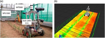
A small 4-wheel autonomous robot with differential steering was used as the carrier vehicle to move the sensors through the crop rows (see Figure 1, a) (Reiser et al., Reference Reiser, Izard, Arellano, Griepentrog and Paraforos2016). A LMS111 2D-LiDAR laser scanner (SICK, Waldkirch, Germany) was used, mounted at a height of 0.58 m, above the ground, pointing downwards at an angle of 30 degrees. The sensor data was assembled with 25 Hz and an angle resolution of 0.5 degrees. This position was selected to allow 3D point cloud generation and at the same time to be able to navigate the robot system with the sensors through the rows. To measure the robot orientation, a VN-100 Inertial Measurement Unit (IMU) (VectorNav, Dallas, USA) was included in the sensor setup. The robot position was obtained through the use of a SPS930 Universal Total Station (Trimble, Sunnyvale, USA). The total station tracked a Trimble MT900 Machine Target Prism, which was mounted on top of the robot at a height of 1.07 m (see Figure 1, a).
The robot platform for the data acquisition (a) and the visualization of the robot in the Robot Operating System (ROS) with one assembled point cloud and the ground truth of the plants as green sticks (b).

Software
The robot computer runs on Ubuntu 14.04 and uses the Robot Operating System (ROS-Indigo) middleware for sensor control and data recording. The system could be used for live monitoring of the sensor data and provided the necessary visualization tools (see Figure 1, b). All the software components were programmed in a combination of C++ and Python programming languages. For fast calibration, point measurement and importing the total station data into ROS, the Trimble SCS900 Site Controller (Software Version 3.4.0) graphical interface was used. The prism position data was time stamped and helped to refer the transforms to the global frame and to interpolate the data.
For the plant detection, a ROS node (executable-program) was developed, reading in the assembled point cloud and giving out the results of the algorithm. This implementation could be used directly on a real-time operating robot system. For the specific point cloud algorithms the PCL implementation (Rusu and Cousins Reference Rusu and Cousins2011) was used and optimized for ROS.
Data Acquisition and Point Cloud Assembling
For referencing to the same Cartesian coordinate frame in every test, 5 fixed points were defined nearby the test area (Garrido et al., Reference Garrido, Paraforos, Reiser, Vázquez Arellano, Griepentrog and Valero2015; Reiser et al., Reference Reiser, Izard, Arellano, Griepentrog and Paraforos2016). To relocate these points for every test, a greenhouse with a solid concrete wall was selected for the data acquisition. The precise position of these 5 points could be located by just screwing a prism of the total station on fixed positions on the concrete wall. With these positions, the positioning system of the total station could be calibrated to one fixed coordinate frame. The inaccuracy in the static measurement could be estimated by reassessing each of these fixed points with the first measurement. The shift between the first reference points and the actual measurements was in all tests below 4 mm for all three dimensions. For the robot rigid body frame, carrying the sensors, a static transformation between the prism and the sensor position was assumed. First the roll, pitch and yaw angle of the IMU was fused together with the prism position and was used to create a coordinate frame for the prism position. After that, a static transformation to the robot geometric center and to the sensor position was performed. This procedure allowed to track down the precise sensor position and orientation in the same reference frame in every test (Garrido et al., Reference Garrido, Paraforos, Reiser, Vázquez Arellano, Griepentrog and Valero2015; Reiser et al., Reference Reiser, Izard, Arellano, Griepentrog and Paraforos2016).
The spacing between the plants was defined by different Gaussian distributions for every crop row, to emulate diverse real scenarios. The rows used in this paper had a Gaussian distribution and a standard deviation of 0.02 m and 0.03 m for the spacing. In total 41 plants were planted per row. The ground truth positions of the plants were measured using the total station just after emergence with the help of a tripod.
In total six different growth stages were assessed in this paper, the first test 28 days and the last test 47 days after seeding. The average height of the plants changed in this time between 12.03 cm and 41.76 cm. The absolute plant height was varying between 5.7 and 45 cm. The real height of the plants was measured manually after every test day right after the data acquisition. The plants were between V1 and V6 stage, varying at every test day (Ritchie et al., Reference Ritchie, Hanway and Benson1993).
For the data acquisition the robot drove through the row always from the same side with an average speed of 0.02–0.04 m/s. All six tests were performed in the same row, in the same driving direction, towards the total station. The laser scanner was always at the front of the driving direction.
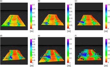
Before assembling the data of the LiDAR into a 3D point cloud, the single scans were filtered with a range filter, so that reflections of the vehicle and the greenhouse wall were removed from the sensor data. The limits of the points were set to a defined distance, so that just one row to the left and one to the right of the robot could be observed. Only the points in the range of 0.75 m to the left and 0.75 m to the right of the sensor position were considered. This filtered scans were transformed together with the fusion of the robot position, gained by the total station and the IMU orientation, into one coordinate system. With this new reference, all points could be transferred to one 3D point cloud, in one global world coordinate system. In Figure 2 the 3D assembled point cloud representations in six different grow stages are depicted. The colors represent the height value of the points.
Assembled point clouds used for the algorithm with the six different assessed growth stages: (a) 26, (b) 28, (c) 32, (d) 35, (e) 40 and (f) 47 days after seeding.

Plant detection algorithm
To speed up the detection algorithm and get more precise results, the area of interest (AOI) was defined around the single particular plant, just taking one square meter around the plant into account. To test the limits of the algorithm, no noise reduction was applied. Limiting the AOI around the single particular plant, allowed to create a more precise estimation of the data points representing the soil. As the shape of the ground was roughly planar in the data set, a random sample consensus (RANSAC) based plane fitting algorithm was used to remove the points of the ground (Fischler and Bolles Reference Fischler and Bolles1981) and separate them from the plant points.
The plant points in the AOI were afterwards clustered to define point cloud groups of every single plant with the use of the ground truth of the plant position. A graph-cut based algorithm was used to cluster the plant points (Boykov and Funka-Lea Reference Boykov and Funka-Lea2006). This method fits perfect to the described problem, as it allows to separate foreground and background objects by using the known position of the object of interest. Compared to the use in 2D image analysis, the graph-cut based algorithm in point clouds cannot use color information to define the nodes and edges of the graph. The only possible organizing methods for the graph are distances and densities between the points. Therefore, the point cloud was organized in a k-nearest neighbor graph, using the row direction as separator (Bentley Reference Bentley1975), correlating with the X-Axis in the point cloud reference frame (Reiser et al., Reference Reiser, Izard, Arellano, Griepentrog and Paraforos2016). Every point of the point cloud was defined as a node of the graph. This defined graph was then clustered with a min-cut in foreground and background points (Golovinskiy and Funkhouser Reference Golovinskiy and Funkhouser2009). For that, it is necessary to define sink and source points to set the edges, linking the nodes (points) of the graph. The source points define the assumed center of the object of interest. The sink points define background points. The edge value defines the weight that is used for the min-cut clustering. This weight decreases with the distance to the source point. The weight w i of edge i is defined with the distance d i to the source point and the additional fixed parameter σ.
 $$w_{i} =e^{{{\minus}\left( {{{d_{i} } \over \sigma }} \right)^{2} }} $$
In this case, the real plant position was used as source point with a predefined source weight as starting weight value. As sink points, all points with a distance radius area around 0.5 m around the real plant position were defined. The final segmentation was done by minimizing the cut cost of the nearest neighbor graph and the background penalty (Golovinskiy and Funkhouser Reference Golovinskiy and Funkhouser2009).
To assess the clustering, first the minima and maxima points of the gained point cloud were assessed. When the ground plane is shown with the point-normal form, the minimal distance h i between a point P i (x i , y i , z i ) to a plane can be defined as:
 $$h_{i} =ax_{i} {\plus}by_{i} {\plus}cz_{i} {\plus}d$$
with a,b,c,d defining the plane equation parameters. As the parameters a and b converged to zero and parameter c converged to one, the estimated height was approximated with h=z+d. The stem position was approximately estimated with the 3D centroid of all resulting points. The centroid c is correlated to the number of n points p in one point cloud cluster in equation 3.
 $$c={1 \over 3}\mathop{\sum}\limits_{i=1}^n {p_{i} } $$
Just the x and y coordinates of the plants were considered for ground truth. The results of the algorithm for plant positions were compared to the measured positions by the total station to define the achieved precision. The height was compared with the manual measurements taken after every data acquisition. For assessing the accuracy of the plant pose and the height, the mean value
 $$\bar{d}$$
, the standard deviation std
dev
and the Root Mean Square Error (RMSE) were used:
 $$\bar{d}={1 \over N}\sqrt {(x_{r} {\minus}x_{a} )^{2} {\plus}(y_{r} {\minus}ya)^{2} } $$
 $$std_{{dev}} =\sqrt {{1 \over N}{\asterisk}\mathop{\sum}\limits_{i=1}^N {(d_{a} {\minus}\bar{d})^{2} } } $$
 $$RMSE=\sqrt {{1 \over N}\mathop{\sum}\limits_{i=1}^N {\left( {\sqrt {(x_{r} {\minus}x_{a} )^{2} {\plus}(y_{r} {\minus}ya)^{2} } } \right)} } $$
with d r (x r ,y r ) as ideal plant position measured by the total station and d a (x a ,y a ) as the resolved algorithm plant position in 2D and N as the number of assessed datasets.
Results and discussion
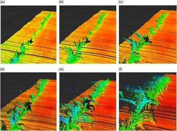
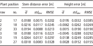
The algorithm was applied to six selected plants. Each was assessed in six different growth stages. For each row three plants were assessed. All plants were grouped in the row with highly overlapping leaves in the later growth stages (see Figure 2). For applying the algorithm, the settings of the adjustable parameters were fixed in all data sets. The only change between each assessment was the definition of the ideal plant position as source point. The used settings were σ=0.5, radius=0.5, source weight=0.25 and the minimal neighbors acceptable with 5 points. The results of the plant 17 in row 2 are shown in the following Figure 3. The results of the stem detection and height estimation of the evaluated six plants with standard deviation and RMSE could be found in Table 1.
Clustered points for plant 17 of row 2 in all six growth stages, black points are the clustered plant points: (a) 26, (b) 28, (c) 32, (d) 35, (e) 40 and (f) 47 days after seeding (V1-V6 (Ritchie et al. Reference Ritchie, Hanway and Benson1993)).

Results of the plant-clustering algorithm combined over all six growth stages

The achieved precision was accurate, so showed the mean value the best deviation of the stem position of 1.88 cm for all six growth stages and reached in some of the measurements even the position accuracy of 0.21 cm. The worst positioning error was 5.19 cm at plant 19 in row 3 what was caused by a partial covering of the plant of one big maize plant just 10 cm away from the examined plant. This caused the much higher RMSE for the stem distance. The poorly results for the plant 27 of row 3 are caused by a general offset to the ground truth, what could be caused by an error while measuring the plant position, or a special shape of the plant, what caused that the center of the plant did not fit with the stem position. Using a more complex model for the stem pose estimation in the point clouds and denser point clouds would bring improvements to the results. The RMSE height estimation ranged for the examined plants between 1.55 and 3.85 cm. The best estimations for single growth stages reached an accuracy of 1.1 mm for plant 33 in row 2 and plant 27 in row 3. The worst detection had an accuracy of 6 cm for one test in row 2 for plant 17. This was caused by not perfectly clustered point clouds, cutting off leaves at the top.
From visual feedback, the ground truth does not match completely with the 3D point cloud plant poses. This could be caused by the inaccuracy of the used LMS111 laser scanner depth information. In the manual the systematic error was described with +/−30 mm with a maximum of +/−50 mm (Sick AG Waldkirch 2016). When visually comparing the algorithm stem positions with the laser scanning data, the results seemed quite accurate. This inaccuracy in the sensor data showed, that the algorithm would be quite robust against not precise plant pose estimations. The algorithm results matched with the sensor data and not with the ground truth points. The algorithm worked well for detecting accurately the stem position of small plants, but it had the tendency to cut off small leaves and not clustering them, when they were too far apart from the assumed center of the object.
Future work should evaluate how precise the plant estimation must be in order to detect precisely the plants and how a known plant spacing could help to perform better results. In addition, the evaluation of all plants in the row should be done to evaluate the robustness of the suggested algorithm with more data. To evaluate the quality of the point clouds and the clustering, the spatial correlation between the clustered point clouds and the leaf area and biomass change could be investigated.
Conclusions
In this work, a mobile robot was used for assembling 2D laser scanner data in six different growth stages of maize plants. The data was assembled to a 3D point cloud and clustered with a graph-cut based algorithm. In total, 6 different plants at 6 different growth stages with a varying height between 5.7 and 45 cm were assessed. It was shown that all plants could be clustered correctly, with the same algorithm settings, when using the previous known plant position. The results were better than the LiDAR sensor accuracy specifications, with accuracies for stem position of 2.02 cm and plant height estimation of 1.55 cm.
Acknowledgments
The project was conducted at the Max-Eyth Endowed Chair (Instrumentation & Test Engineering) at Hohenheim University (Stuttgart, Germany), which is partly grant funded by the Deutsche Landwirtschafts-Gesellschaft e.V. (DLG).