
1. Introduction
Marangoni spreading driven by a surface tension gradient at an interface is ubiquitous in nature, e.g. it explains the dynamics of oil spreading on the sea (Hoult Reference Hoult1972), some living organisms profit from it to achieve self-propulsion (Burton et al. Reference Burton, Cheng, Vega, Andrés and Bush2013) and so on. It is also relevant to industrial processes, e.g. coating (Kim et al. Reference Kim, Boulogne, Um, Jacobi, Button and Stone2016), encapsulation (Koldeweij et al. Reference Koldeweij, van Capelleveen, Lohse and Visser2019) and drying (Matar & Craster Reference Matar and Craster2001). The spreading can be initiated by introducing amphiphilic molecules (Roché et al. Reference Roché, Li, Griffiths, Le Roux, Cantat, Saint-Jalmes and Stone2014) and by evaporation (Dussaud & Troian Reference Dussaud and Troian1998). The latter coupled with de-wetting of a substrate (Zhao et al. 2015; Keiser et al. Reference Keiser, Bense, Colinet, Bico and Reyssat2017; Mouat et al. Reference Mouat, Wood, Pye and Burton2020) provides a methodology for creating spatially ordered patterns and droplets (Yamamoto et al. Reference Yamamoto, Nakajima, Shioi, Krafft and Yoshikawa2015; Wodlei et al. Reference Wodlei, Sebilleau, Magnaudet and Pimienta2018) which are relevant to biomedical applications such as high-throughput screening. The spreading can also occur during deposition of an evaporating droplet on a miscible substrate, facilitating transport while avoiding contamination of immiscible chemicals (Kim et al. Reference Kim, Muller, Shardt, Afkhami and Stone2017). Surfactant-assisted Marangoni spreading has implications for surfactant replacement therapy for newborns suffering from respiratory distress syndrome (Grotberg Reference Grotberg2001). Marangoni spreading also plays a role in airway delivery of antibiotics via inhalation of atomized droplets (Iasella et al. Reference Iasella, Stetten, Corcoran, Garoff, Przybycien and Tilton2018); this is viewed as a potentially low-cost, high-efficiency and low-side-effect drug delivery method for treatment of airway diseases. These applications necessitate determination of the basic mechanisms responsible for the transport of solutes (Iasella et al. Reference Iasella, Sun, Zhang, Corcoran, Garoff, Przybycien and Tilton2019) and particles (Wang et al. Reference Wang, Bonaccurso, Venzmer and Garoff2015; Dunér et al. Reference Dunér, Garoff, Przybycien and Tilton2016) using the deposition of droplets containing either surfactant molecules or lipid dispersions (Stetten et al. Reference Stetten, Moraca, Corcoran, Tristram-Nagle, Garoff, Przybycien and Tilton2016).
The above applications motivated numerous studies of the dynamics of surfactant- assisted spreading, which determined the spreading rate, the shape of the liquid–air interface with a distribution of amphiphilic molecules on it and the onset of the fingering instability developed at the periphery (Afsar-Siddiqui et al. Reference Afsar-Siddiqui, Luckham and Matar2003a,Reference Afsar-Siddiqui, Luckham and Matarb; Matar & Craster Reference Matar and Craster2009). Jensen & Grotberg (Reference Jensen and Grotberg1992) predicted theoretically, by considering the mass conservation of the surfactant molecules, that the radius of a spreading droplet with an insoluble surfactant increases with time t proportionally to  ${t^{1/4}}$; this exponent increases to 1/2 when a continuous supply of surfactants is available (Borgas & Grotberg Reference Borgas and Grotberg1988). The spreading rate can be adjusted by changing the thickness (Troian, Wu & Safran Reference Troian, Wu and Safran1989) and viscosity (Bacri, Debrégeas & Brochard-Wyart Reference Bacri, Debrégeas and Brochard-Wyart1996) of the substrate, and by the adsorption of molecules at a liquid–solid interface (Nikolov et al. Reference Nikolov, Waan, Chengara, Koczo, Policello and Kolossvary2002).
Marangoni spreading leads to large interface deformations including the formation of a Marangoni ridge whose position corresponds to the location of the leading edge of the spreading surfactant, as well as the formation of a severely thinned region upstream of the ridge (Troian, Herbolzheimer & Safran Reference Troian, Herbolzheimer and Safran1990). The quantitative description of the spreading process involves a system of coupled partial differential equations describing the liquid depth and the concentration distribution of surfactants at the interface (Gaver & Grotberg Reference Gaver and Grotberg1990). Solutions accounting for a multitude of effects such as surface diffusion and capillarity (Matar & Troian Reference Matar and Troian1997; Warner et al. Reference Warner, Craster and Matar2004a), solubility (Warner et al. Reference Warner, Craster and Matar2004b) and intermolecular forces (Matar & Troian Reference Matar and Troian1999) reveal a fingering instability at the severely thinned region. The occurrence of this instability was confirmed by numerous experiments (Troian et al. Reference Troian, Wu and Safran1989; Cachile & Cazabat Reference Cachile and Cazabat1999; Cachile et al. Reference Cachile, Schneemilch, Hamraoui and Cazabat2002) which also demonstrated a correlation between the disturbance wavelength and the film thickness (Afsar-Siddiqui et al. Reference Afsar-Siddiqui, Luckham and Matar2003b; Keiser et al. Reference Keiser, Bense, Colinet, Bico and Reyssat2017). The body (Pearson Reference Pearson1958) and surface (Czechowski & Floryan Reference Czechowski and Floryan2001) modes of Marangoni instability, i.e. convective rolls established in the liquid layer due to a surface tension gradient at the interface, are not expected to play a role due to the rapidity of the spreading process. The interface rupture is yet to be investigated in detail (Floryan & Chen Reference Floryan and Chen1994).
The understanding of Marangoni spreading on Newtonian substrates may not be sufficient for explaining the airway drug delivery process as the substrate has high viscosity and complex rheology. The airway surface consists of a layer of mucin on top of a layer of cilia and tethered macromolecules, whose properties can be described using a viscoelastic model (Stetten et al. Reference Stetten, Iasella, Corcoran, Garoff, Przybycien and Tilton2018a). The first experimental investigations in this area are due to Koch et al. (Reference Koch, Dew, Corcoran, Przybycien, Tilton and Garoff2011) and Stetten et al. (Reference Stetten, Treece, Corcoran, Garoff, Przybycien and Tilton2018b). Theoretical investigations revealed that the presence of mucus affects the interface shape and the surfactant distribution during spreading, as well as rupture of the film if van der Waals forces are present (Matar, Craster & Warner Reference Matar, Craster and Warner2002). Theoretical analysis of the spreading dynamics on a weakly viscoelastic substrate film modelled as an Oldroyd-B fluid suggested the importance of streamwise normal stress as well as the shear stress in the spreading process (Zhang et al. Reference Zhang, Matar and Craster2002).
The above studies were focused on axisymmetric spreading. Some experiments involving films with stronger viscoelastic properties reported the formation of finger-like, non-axisymmetric modulations at the contact line between the droplet, substrate and air (Motaghian et al. Reference Motaghian, van Esbroeck, van der Linden and Habibi2022; Ma et al. Reference Ma, Zhong, He, Liu and Li2020). These observations suggested the existence of a new class of interfacial elastic instability similar to the one observed by Grillet, Lee & Shaqfeh (Reference Grillet, Lee and Shaqfeh1999) in their experiments with viscoelastic fluids confined between eccentric cylinders displacing the less viscous fluid (the air). A thorough study is required to determine the onset conditions and the character of the amplified disturbances during spreading on films made of viscoelastic liquids.
It is known that viscoelasticity plays an important role in the interface dynamics. Viscous fingering results from an instability developed at the interface between two immiscible fluids confined in a Hele–Shaw cell with the less viscous fluid displacing the more viscous fluid if the capillary number exceeds a critical value (Saffman & Taylor Reference Saffman and Taylor1958; Homsy Reference Homsy1987). Viscoelasticity was shown to affect the finger width through the first normal stress difference  ${N_1}$ caused by the high shear rate in the liquid film (Lindner et al. Reference Lindner, Bonn, Poiré, Amar and Meunier2002). Fingers were replaced by a ribbing instability when unconfined geometries were of interest as observed in the case of the air–liquid interface during the roll-coating process (Sullivan & Middleman Reference Sullivan and Middleman1979; Bauman, Sullivan & Middleman Reference Bauman, Sullivan and Middleman1982); it is known that the elastic effect at curved streamlines was responsible for the destabilization (Grillet et al. Reference Grillet, Lee and Shaqfeh1999). A theoretical study (Graham Reference Graham2003) revealed the mechanism of the ribbing caused by hoop stresses at a curved interface. A height perturbation of the free surface led to a local accumulation of normal stress, which further amplified the perturbations. The disturbance wavelength was found to be of the order of the film thickness, both for Newtonian and viscoelastic fluids. However, the instability growth rate of the viscoelastic fluid was much higher than that for Newtonian fluids, leading to the formation of easily observable ribs in the case of viscoelastic fluids. Viscoelasticity also affects the contact line dynamics. In a dip-coating and withdrawing experiment, viscoelasticity was found to alter the way the dynamic contact angle depends on the capillary number Ca (Kim & Rothstein Reference Kim and Rothstein2015). Viscoelasticity was shown to play a stabilizing role for advancing contact lines with a fixed contact angle. In the experiments of droplet spin-coating, viscoelasticity delayed the onset and decreased the wavenumber of the contact line instability (Spaid & Homsy Reference Spaid and Homsy1997). Viscoelasticity was shown to play a destabilizing role in the receding contact line dynamics, such as for fluid confined between eccentric cylinders exposed to shear flow (Grillet et al. Reference Grillet, Lee and Shaqfeh1999); in this case, fingers can be produced at the fluid–air interface for both the Newtonian and viscoelastic fluids. However, if viscoelastic effects are present, a further increase of Ca leads to the appearance of hoop stresses at the round fingers, which causes the fingers to evolve into cusp-like configurations, a phenomenon not observed in Newtonian fluids. In the blade-coating experiment of Deblais et al. (Reference Deblais, Harich, Colin and Kellay2015), a cusp-like pattern formed at the receding contact line in a certain range of Ca. Although cusps were observed in Newtonian fluids, e.g. droplets running down along an inclined surface (Podgorski, Flesselles & Limat Reference Podgorski, Flesselles and Limat2001; Limat & Stone Reference Limat and Stone2004), cusps can also evolve into filament-like patterns for viscoelastic fluids whose shape is similar to the recently observed patterns during Marangoni spreading on viscoelastic fluids (Motaghian et al. Reference Motaghian, van Esbroeck, van der Linden and Habibi2022; Ma et al. Reference Ma, Zhong, He, Liu and Li2020). Shearing and curved streamlines, which are known to be important for the creation of the elastic instability, can be found in Marangoni spreading, and may lead to instability phenomena which do not occur in Newtonian fluids. To the best of our knowledge, there are very few experimental studies dealing with the flow dynamics and instability of Marangoni spreading on a viscoelastic substrate.
We report in this paper results of experimental investigations of Marangoni spreading of surfactant-laden droplets made of a Newtonian liquid deposited on more viscous Newtonian and viscoelastic thin films. We study the dynamics of spreading, with a focus on the effect of liquid elasticity. The elasticity creates an instability at the contact line which correlates with the pattern of interface deformation which is different from what is observed for Newtonian fluids. Particle tracking velocimetry (PTV) is used to investigate the flow field in the liquid film during spreading. PTV and the transmission-speckle method are used to determine the three-dimensional morphology of the film–droplet interface.
2. Experiments
2.1. Solutions used in the experiments and rheology
The aqueous solutions of polyethylene glycol (PEG) 8 kDa and polyethylene oxide (PEO) 8 MDa (from Sigma-Aldrich) were made by dissolving polymer powders in deionized water (from Shanghai Titan Scientific Co.). The container was prewetted with deionized water, then powders were dispersed on the side walls while the container was rotated manually to provide their uniform distribution. A fixed volume of deionized water was added into the container and homogeneous solutions were obtained through magnetic stirring at 100 rpm at room temperature for 7 days. Two viscoelastic Boger fluids (Dontula, Macosko & Scriven Reference Dontula, Macosko and Scriven1998) were made by mixing 33.4 weight ratio (wt%) of PEG solution with 0.16 wt% of PEO solution, and by mixing 16.7 wt% of PEG solution with 0.08 wt% of PEO solution. The viscoelastic properties of both fluids were characterized using a rheometer (Anton Paar MCR302) with 15° cone-plate rotor (CP50-1) at shear rate varying from 0.1 s−1 to 1000 s−1 at 25 °C. The measured viscosity shown in figure 1 demonstrates that the shear thinning was not significant in the range of shear rates used in the experiment. The viscoelastic relaxation times  $\tau $ of Boger fluids were determined using the Oldroyd-B model (Lindner et al. Reference Lindner, Bonn, Poiré, Amar and Meunier2002) in the form
 ${N_1} = {\varphi _1}\; {\dot{\gamma }^2}$, where
 $\dot{\gamma }$ stands for the shear rate and
 $\varphi$1 denotes the first normal stress difference coefficient defined as
 $\varphi$1 =
 $2N{k_B}T{\tau ^2}$. Here, N is the number density of the polymer (number of PEO molecules per unit volume of the solution),
 ${k_B}T$ is the thermal energy,
 ${k_B}$ is the Boltzmann constant and T stands for the temperature. Values of
 $\varphi$1 were determined from the dependence between
 ${N_1}$ and
 $\dot{\gamma }$ measured experimentally (see figure 1). We shall use symbol
 ${\tau _\phi }$ to identify the relaxation time determined in this manner. The relaxation time can also be determined from the known viscosity using the relation
 $\eta = {\eta _s} + N{k_B}T\tau $, where
 $\eta $ is the viscosity obtained from figure 1 and
 ${\eta _s}$ is the viscosity of the PEG solvent;
 ${\tau _\eta }$ is determined as
 $(\eta - {\eta _s})/N{k_B}T$, where symbol
 ${\tau _\eta }$ is used to denote relaxation time determined in this manner. We have also carried out experiments using PEG solutions to provide a reference case of spreading on Newtonian fluids for comparisons with spreading on Boger fluids; PEG solutions have the same monomers as Boger fluids, except the molecular length. We used sucrose (from Rhawn Co.) solutions at different concentrations to study the onset condition for formation of patterns during spreading on Newtonian fluids. The viscosities of these solutions and the calculated viscoelastic relaxation times are given in table 1. Surfactant solution was made by diluting the non-ionic surfactant Triton X-100 (from Beijing Solarbio Science & Technology Co. Ltd) to avoid reactions of ionic surfactants with the polymers (Smitter et al. Reference Smitter, Guédez, Muller and Saez2001). The critical micelle concentration (cmc) of Triton X-100 is 0.01229 wt%. Droplets with 40 cmc Triton solution, corresponding to a surface tension of 31.4 mN/m, were used in all experiments. The refractive index of Boger fluids is 1.358 and that of the surfactant-laden droplets is 1.33, measured by a refractometer (Atago DR-A1).
Variations of viscosity  $(\eta )$ and the first normal stress difference
 $({N_1})$ of the substrate fluid as functions of the shear rate
 $\dot{\gamma }$. Symbols represent experimental points and continuous lines represent correlations determined using the least squares method and constrained to represent a parabola. Blue and red colours represent different Boger fluids and black colour represents PEG solution (Newtonian fluid).

Viscosity  $\eta $ and viscoelastic relaxation times
 $(\tau )$ of solutions used in this study. Here,
 ${\tau _\phi }$ was obtained from the Oldroyd-B model (Lindner et al. Reference Lindner, Bonn, Poiré, Amar and Meunier2002) (see text for details) and
 ${\tau _\eta }$ was determined from measured viscosity
 $\; \eta $ (see text for details). Symbol ‘Suc’ indicates sucrose solution with the number next to it denoting concentration. All measurements were carried out at 25 °C.

2.2. Creation of films and droplet deposition
The process of creation of a thin film made of either a Newtonian or a Boger liquid started by rinsing the glass base with ethanol (from Shanghai Titan Scientific Co.), drying it using Kim wipes and then cleaning it with plasma cleaner (Harrick Plasma PDC-32G-2) for 35 seconds resulting in a hydrophilic surface. Since the high hydrophilicity can be sustained in air only for a short period, the liquid (0.15 ml) was placed on the glass base within 20 seconds of completion of plasma treatment and its spreading was assisted by tilting the base in all directions producing a thin film with an area of approximately 10 cm2. The excess liquid (of the order of 0.1 ml) was removed using a micropipette (Eppendorf 100–1000 μl) leaving approximately 0.05 ml of the liquid on the glass. The film will begin to retract if the spreading parameter  $S = {\gamma _{sv}} - {\gamma _{sl}} - \gamma$ is negative (de Gennes, Brochard-Wyart & Quéré Reference de Gennes, Brochard-Wyart and Quéré2002), which was the case in our experiment. Here,
 ${\gamma _{sv}}$ denotes the surface tension between the solid and the vapour,
 ${\gamma _{sl}}$ stands for the surface tension between the solid and the liquid, and
 $\gamma $ denotes the surface tension between the liquid and the vapour. The retraction velocity V of the contact line for viscous fluid is
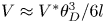 $V \approx {V^\mathrm{\ast }}\theta _D^3/6l$ (de Gennes et al. Reference de Gennes, Brochard-Wyart and Quéré2002), where
 ${V^\mathrm{\ast }}$ scales with
 $\gamma /\eta $ signifying competition between the surface tension which drives the retraction and the viscous dissipation which opposes the retraction,
 $l \approx 20$ is a dimensionless coefficient, and
 ${\theta _D}$ is the dynamic contact angle at the receding contact line. We estimated the retraction velocity in our experiments to be of the order of
 $0.01\;\textrm{mm}\;{\textrm{s}^{ - 1}}$ for viscous solution with
 $\eta \; = 22\;\textrm{mPa}\ \textrm{s}^{-1}$ and
 $\gamma \approx 31.4\;\textrm{mN}\;{\textrm{m}^{ - 1}}$. To account for the retraction (de-wetting) effect, the experiment (droplet deposition) started within 30 sec of formation of the film and the area covered by the film and the film thickness was measured at the time of droplet deposition.
During experiments, the time was counted from the moment of surfactant deposition onto the film. Droplets with a volume of  $13\;\mathrm{\mu }\textrm{l}$ were used and were deposited using a syringe pump (LonggerPump Co.) with its nozzle placed 4 mm above the film; no splashing was observed.
2.3. Light transmission method and PTV
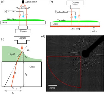
The light transmission method was used to observe the droplet spreading with a viewing zone of approximately 20 mm diameter, with illumination from above provided by a xenon light (HDL-II 470VA, Suzhou Beitejia Photoelectric Technology Co.), and with the spreading recorded from below at 250 frames per second (fps) for spreading on PEG films and 125 fps for spreading on Boger films using a fast camera (Photron SA5); see figure 2(a) for a typical setup and figure 3(a) for typical results. Variations of grey intensity are related to deformation of the film–droplet and the droplet–air interfaces with the image analysis unable to distinguish between them. Other measuring techniques were required to make this distinction; these issues are discussed later in this presentation. The transmission method provides a means for a qualitative observation of morphology of the interfaces and for identification of differences between spreading on the Boger and Newtonian films; it also provides means for quantification of these effects when combined with other measuring techniques.
Experimental setup used for observation of droplet spreading. (a) Schematic diagram of the light transmission method. (b) Schematic diagram of the transmission-speckle method; a plastic sheet with a regular pattern (i.e. lattice) is placed under the liquid container with the red layer indicating the LED illumination. (c) Sketch of the LED light path for the transmission-speckle method; light is refracted at the glass–liquid boundary, and then refracted again at the liquid-air interface. (d) Speckles’ virtual deformation pattern observed during spreading; the red line identifies the quarter-circular zone used in the analysis.

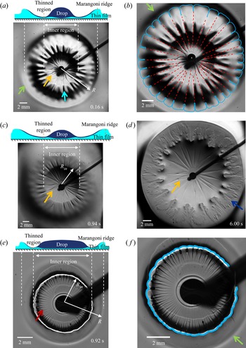
Images of spreading of surfactant-laden droplet with  $\eta = 1\;\textrm{mPa}\ \textrm{s}^{-1}$. (a) Droplet position during spreading on the Boger 2 (see table 1 for its properties) liquid film with thickness
 ${h_0} = 85\;\mathrm{\mu }\textrm{m}$ at time t = 0.16 s; orange arrow points to the rib-like patterns; blue arrow points to the interface corrugation patterns; green arrow points to the position of the spreading front (Marangoni ridge), the position of the outer edge of the wide fingers very close to the Marangoni ridge is identified using the spreading radius R. (b) Copy of panel (a) with a blue line marking the contact line and showing the formation of wide fingers, and a red dashed line identifying the rib-like patterns with the same wavenumber as the fingers. (c) and (d) Droplet's positions at times t = 0.94 s and t = 6 s, respectively; the rib-like patterns can be observed; blue arrow points to the highly stratified fingers in the thinned zones upstream of the Marangoni ridge. (e) Spreading of an identical droplet on a Newtonian PEG fluid (see table 1) with viscosity similar to the viscosity of the ‘Boger 2’ fluid and with the film thickness
 ${h_0} = 89\;\mathrm{\mu }\textrm{m}$ – position of the droplet at time t = 20 ms; red arrow points to the radial patterns. ( f) Copy of panel (e) with a blue line marking the position of the wavy contact line without any fingers. See text for other details.

Detailed observation of the same phenomenon with a viewing zone of approximately 4 mm in diameter and recording rate of 7000 fps were carried out using a reversed transmission microscope (Nikon Ti2-U), which was used to track particle movements in the film seeded with 10 μm diameter polystyrene particles (DaE Tianjin Technology Co.) and to provide data for the PTV. The ‘nearest neighbour’ method was used to determine position of particles in two successive images (Li et al. Reference Li, D'eramo, Lee, Monti, Yonger, Tabeling, Chollet, Bresson and Tran2015) to determine particle velocities.
2.4. Transmission-speckle method
The principle of the transmission-speckle method can be explained using geometric optics. Speckles are placed under the fluid container. An LED panel (OPT-DPA, 48 W) provides illumination from the bottom with light rays penetrating through the glass base and through the liquid film, as shown in figure 2(b). Light is refracted at the glass–film boundary, then at the film–droplet interface and again at the droplet–air interface. Since the refractive indices of the Boger film  $({n_B} = 1.358)$ and the spreading droplet
 $({n_d} = 1.33)$ are very similar, we neglect the light refraction at the film–droplet interface, and only account for the refraction at the glass–film boundary and the droplet–air interface (see figure 2c). The resulting bias in the measurements of deformation of the droplet–air interface is discussed in § 3.5. The refraction pattern was captured by a camera placed above the liquid. When a deep layer and thin base were used, the virtual displacement induced by refraction at the solid–liquid boundary was negligible compared to the refraction at the droplet–air interface. The method is well established for such conditions and was used to measure the profile and evolution of surface waves with an accuracy of approximately 1 μm (Shi, Huang & Liu Reference Shi, Huang and Liu2014). A similar method was applied to measure the shape of the interface during droplet spreading on a deep liquid layer and to capture azimuthal variations of the interface near the contact line resulting from the fingering instability (Ma et al. Reference Ma, Zhong, He, Liu and Li2020). Speckles were created by printing regular lattices on plastic sheets; black lines orthogonal to each other and spaced 0.1 mm apart were printed, creating a pattern of transparent spots. The speckle virtual displacement was analysed using digital image correlation (DIC) (Helm Reference Helm2008; Wang et al. Reference Wang, Wu, Kang, Wang, Li, Hou, Riaz, Li and Li2019). The principle of the DIC method is to find matching regions with precise locations between the reference image and the target image using a correlation function resulting in determination of the speckles displacement field. A multi-directional Newton iteration algorithm was used to determine the relation between the speckle virtual displacement and the liquid height (Shi et al. Reference Shi, Huang and Liu2014). A known height at an unaffected region, given as a sum of the glass base thickness and the initial film thickness, was used to initiate computations.
In this work, we investigate the deformation of the droplet–air interface during droplet spreading on very thin films; the typical film thickness was less than 100 μm, i.e. it was much smaller than the thickness of the glass base (1.85 mm). The physical situation is different from those reported in the literature as refraction at both the droplet–air interface and the solid–liquid interface must be considered. In our experiment, we take advantage of the small incident angle  $\beta $ and small refractive angle
 $\alpha $ at the solid–liquid boundary, as shown in figure 2(c); we neglect possible refraction at the film–droplet interface as discussed previously. According to Snell's law,
 ${n_l}\sin (\alpha ) = {n_s}\sin (\beta )$, where
 ${n_l}$ denotes the refractive index of liquid and
 ${n_s}$ stands for the refractive index of glass. The actual speckle in-plane virtual displacement S is expressed as
 $S = {h_1}\tan (\alpha ) + {h_2}\tan (\beta )$. The apparent displacement with refraction at the solid–liquid boundary omitted is
 ${S_l} = ({h_1} + {h_2})\tan (\alpha )$. Use of the small-angle approximation leads to
 $\tan (\alpha ) \approx \alpha $,
 $\tan (\beta ) \approx \beta $,
 ${S_l} \approx \textrm{(}{h_1} + {h_2}\textrm{)}\alpha$ and
 $S \approx {h_1}\alpha + {h_2}\beta \approx \textrm{(}{h_1} + {n_l}{h_2}/{n_s}\textrm{)}\alpha $. When the liquid film is much thinner than the glass base, i.e.
 ${h_1} \ll {h_2}$, further simplification leads to
 ${S_l} \approx S{n_s}/{n_l}$. In other words, the observed displacement S can be converted to an apparent displacement
 ${S_l}$ by assuming that the glass has the same optical properties as the liquid. Determination of the interface height based on
 ${S_l}$ relies on a multi-directional Newton iteration algorithm (Shi et al. Reference Shi, Huang and Liu2014). The accuracy of this method is approximately 0.1 μm; it depends on the speckle image scale (10 μm pixel−1) and the resolution of the DIC which is better than 0.1 pixels. The camera must be placed facing the liquid surface to have the light reflected perpendicularly into it; misalignment of the camera may result in a systematic error in the height measurements but, nevertheless, the resulting image still captures the main features of the interface shape.
The transmission-speckle method properly captures the interface shape as we were able to identify radial shape variations including the formation of a Marangoni ridge and thinning of the liquid layer behind the ridge similar to those reported in the literature on droplet spreading on viscoelastic films (Zhang, Matar & Craster Reference Zhang, Matar and Craster2002). We are also able to observe the shape variations in the azimuthal direction which was not reported previously; these results will be discussed in § 3.5.
3. Results and discussion
3.1. Patterns formed on the interface during Marangoni spreading
Marangoni spreading driven by surface tension difference occurs immediately after contact between the droplet and the film. The main body of the droplet remains near the contact point with a small amount being spread along the interface; see sketch in figure 3(a) showing the position and approximate shape of the spreading droplet and the film. The characteristic quantities are: (i) the radius of Marangoni ridge  ${R_M}$ giving position of the top of the ridge; (ii) the spreading radius
 $R$, which gives position of the outer edge of wide fingers (see figure 3a;
 $R < {R_M}$); and (iii) the radius of the inner region
 ${R_{in}}$, which is defined as the location where a combination of the liquid film and the spreading droplet has the smallest thickness, and this occurs slightly downstream from the edge of the main body of the droplet (see figures 3c and 3e). In what follows, the inner region corresponds to
 $r < {R_{in}}$, while the outer region corresponds to
 $r > {R_{in}}$. The reader may note that
 $R = {R_M}$ when fingers are not present. The spreading parameter in the experiment was
 $S = {\gamma _B} - {\gamma _d} = 29.2\;\textrm{mN}\;{\textrm{m}^{ - 1}}$, where
 ${\gamma _B}$ and
 ${\gamma _d}$ stand for surface tensions of the Boger fluid and the droplet, respectively. Results displayed in figure 3(a) and in the supplementary movie S1 available at https://doi.org/10.1017/jfm.2023.108 demonstrate that the interface deformation has a form of a wave propagating radially outwards, like the Marangoni ridge observed in spreading on Newtonian films, leaving a severely thinned region for r slightly larger than
 ${R_{in}}$ (Jensen & Grotberg Reference Jensen and Grotberg1992).
Finger formation (see figure 3a), like that previously reported for Marangoni spreading on thick layers of viscoelastic and shear thinning polymer solutions (Ma et al. Reference Ma, Zhong, He, Liu and Li2020), was observed. These fingers were formed by the normal stress which was created by the strong shear resulting from the Marangoni effect at the interface. The fingers’ wavelength selection process was dominated by an elastic deformation near the contact line, with the normal stress difference  ${N_1}$ driving this deformation and the shear elastic modulus
 $G = \eta /\tau $ opposing it. The wavelength was found to increase with an increase of the length scale
 ${({N_1}/G)^{1/2}}$. Similar fingers were found in thin layers of polymer solution during blade coating on a solid surface in the vicinity of the receding contact lines (Deblais et al. Reference Deblais, Harich, Colin and Kellay2015) with their wavelength
 $\lambda $ increasing with an increase of the blade velocity V, e.g.
 $\lambda \sim {V^{3/4}}$, and this is different from the Saffman–Taylor instability where wavelength decreases with an increasing velocity.
In the blade-coating problem (Deblais et al. Reference Deblais, Harich, Colin and Kellay2015), a drop of polymer on a solid surface was sheared by a blade in one direction. The receding contact line developed an instability, which was amplified by the elastic extensional property to form patterns, and the onset of the patterns occurred for capillary number  $Ca = \eta V/\gamma $ ranging from
 ${10^{ - 3}}$ to
 ${10^{ - 1}}$, with
 $\eta $ and
 $\gamma $ being the viscosity and the surface tension of the polymer solution, respectively, and V standing for the blade-coating velocity. In our work, the polymer thin film was sheared by the droplet spreading on top of this film playing the same role as the blade in the blade-coating problem. A significant amount of polymer in the film was expelled radially outwards by the spreading droplet. The wide fingers (see figure 3b) are likely a result of an instability at the film–droplet–air contact line amplified by the elastic property of the Boger fluid.
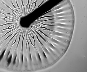
During the initial stages of spreading, when the spreading velocity is large and the shear effects are strong, abrupt azimuthal variations of the interface height were observed in the inner region forming rib-like patterns identified by the dark and light grey zones (see figures 3a and 3c). A typical rib is indicated by the orange arrow and their pattern is marked in figure 3(b) using red dashed lines. As the spreading progresses, gentle wavy azimuthal corrugations form in the outer region (see figures 3a and 3c) leading to the formation of wide fingers at the contact line. A typical corrugation is indicated by a blue arrow in figure 3(a) and the finger pattern is marked in figure 3(b) using a blue line. The ribs form after approximately 10 ms from the moment of deposition which suggests that the Marangoni time scale governs their evolution. The ribs remain visible for up to 10 sec. The rib-like structures were not observed during spreading on thick polymer layers as the interface height perturbations were suppressed by circulation beneath the interface convecting the liquid from the interior of the layer to the interface (Kim et al. Reference Kim, Muller, Shardt, Afkhami and Stone2017). Height perturbations in a thin film cannot be suppressed since there is no recirculation in the interior of the film. Our observations of spreading on a thin film of Boger fluid demonstrate that the appearance of the rib-like patterns is correlated with the instability of the film–droplet–air contact line and is sustained by the small film thickness.
The formation of ribs and wide fingers requires discussion. These structures form because of the elastic properties of liquid activated by shear. In the absence of shear, polymer chains form coils suspended in water. Shear stretches these coils in the shear direction resulting in the formation of an opposing recoiling force within the polymer coil (Oswald Reference Oswald2009). When the viscoelastic liquid film is sheared by the spreading droplet, the recoiling force generates normal stresses acting in the direction of shear (radial direction) and this leads to both the azimuthal variations of the spreading velocity and the azimuthal variations of the contact line (contact line instability). The normal-stresses-driven liquid slowdown in certain azimuthal positions results in the formation of radial ribs. The contact line instability is not a necessary condition for the rib formation as it is known that ribs can be formed just by streamline curvature (Graham Reference Graham2003). The contact line instability does not need the rib formation as a necessary condition either as the contact line instability was found to occur on a deep layer of polymer solution without ribs (Ma et al. Reference Ma, Zhong, He, Liu and Li2020).
The rib-like patterns need to be distinguished from the previously reported fingering instabilities caused by the Marangoni spreading on thin films (Troian et al. Reference Troian, Wu and Safran1989) – these patterns are characterized by formation of multiple very short fingers like those identified by blue arrow in figure 3(d) – we shall refer to such configurations of a short thin finger as stratified fingers. The stratified fingers undergo a transient growth which can be enhanced by Van der Waals forces (Matar & Troian 1999). Such stratified fingers can be observed in our experiments with viscoelastic film if we deposit a second droplet of surfactant solution immediately following deposition of the first droplet. The stratified fingers are different from the radial ribs. They can be observed after approximately 5 s from the droplet deposition; this time scale is more than one order of magnitude longer than the time scale governing rib formation.
To illustrate the role of viscoelasticity in the formation of the rib-like patterns, we carried out a similar experiment with the Boger fluid replaced by a Newtonian fluid (PEG solution) with a similar viscosity (21.5 mPa s‒1; see table 1) and similar film thickness (89 μm). Wide fingers were not observed, as shown in figure 3(e); the contact line marked in blue in figure 3( f) has a wavy shape but without fingers like those observed in the Boger fluid (compare figures 3b and 3f). Radially aligned patterns are clearly visible in the inner region; a typical structure is identified by a red arrow in figure 3(e). These structures are characterized by wavenumbers larger than the wavenumbers for the rib-like patterns on a viscoelastic film (see figure 3a) which suggests different physical origins of both patterns. In the case of Newtonian fluids and a less viscous surfactant solution  $(\eta = 1\;\textrm{mPa}\ \textrm{s}^{-1})$ spreading on a more viscous film, we observed that the radially aligned patterns (such as those displayed in figure 3e) form if the liquids have a sufficiently large viscosity difference and the films are sufficiently thin. This is like the Saffman–Taylor instability in a confined Hele–Shaw channel where a fingering instability occurs when a less viscous fluid pushes against a more viscous fluid. In the next paragraph, we shall discuss the critical conditions required for formation of the radially aligned height perturbations during spreading on Newtonian films with a sufficiently large viscosity difference. This will provide a reference point for identification of differences in spreading caused by viscoelastic effects.
3.2. Spreading on a Newtonian thin film with a large viscosity difference between the droplet and the film
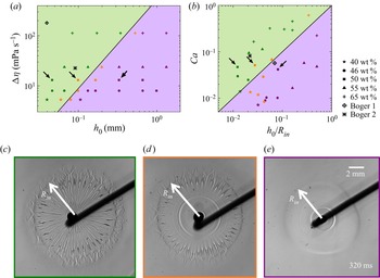
We have carried out a set of experiments on Marangoni spreading of surfactant-laden droplets on thin films made of sucrose solution (Newtonian fluid) with various viscosities and thicknesses. We recorded conditions leading to the formation of the radially aligned patterns, such as those indicated by a red arrow in figure 3(e); the droplet viscosity used to create this image was 1 mPa s‒1 and the viscosity of the film was 21.5 mPa s‒1.
Figure 4(a) displays a phase diagram in the  $(\mathrm{\Delta }\eta ,{h_0})$ plane, where
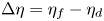 $\mathrm{\Delta }\eta = {\eta _f} - {\eta _d}$ is the viscosity difference with
 ${\eta _f}$ and
 ${\eta _d}$ standing for the viscosity of the film and the viscosity of the droplet, respectively, and
 ${h_0}$ denotes the initial film thickness. For the same
 ${h_0}$, the radially aligned patterns appear if the viscosity difference is larger than critical. When the viscosity difference is constant, the film thickness needs to be smaller than the critical for formation of these patterns. Figure 4(c) displays a typical image when the interface is unstable with the radially aligned patterns being clearly visible, figure 4(d) displays a typical image from the intermediate case when part of the interface is unstable with the radially aligned patterns visible only away from the central point (point of droplet deposition), and figure 4(e) displays a typical image when the interface is stable and no radially aligned patterns exist.
Phase diagrams identifying conditions leading to the formation of stable and unstable interfaces during Marangoni spreading of a less viscous droplet on a more viscous Newtonian thin film. (a) Phase diagram in the  $(\mathrm{\Delta }\eta = {\eta _f} - {\eta _d},{h_0})$-plane; green colour identifies conditions leading to an unstable interface with radially aligned patterns; purple colour identifies conditions leading to a stable interface; orange colour identifies conditions corresponding to the partially unstable cases. Data for the Boger 1 and Boger 2 fluids are included; the rib-like patterns were observed for both fluids. Black arrows identify conditions corresponding to experiments displayed in figure 4(c) (unstable region), figure 4(d) (partially unstable region) and figure 4(e) (stable region). Data used in panels (a) and (b) were collected at 10 ms, whereas data used in panels (c–e) were collected at 320 ms to have instability features more pronounced for better identification of stability regimes. (b) Phase diagram in the
 $(Ca,{h_0}/{R_{in}})$-plane; colours have the same meaning as in panel (a). (c) A typical image of an unstable interface. (d) A typical image of a partially unstable interface. (e) A typical image of a stable interface.
 ${R_{in}}$ stands for the diameter of the inner region.

The same experimental data were re-plotted in figure 4(b) in the  $(Ca = \mathrm{\Delta }\eta \; U/\gamma ,\;{h_0}/{R_{in}})$-plane. Here,
 $\gamma ( = 31.4\;\textrm{mN}\;{\textrm{m}^{ - 1}})$ is the surface tension of the surfactant-laden droplet and U is the velocity characterizing the growth of
 ${R_{in}}$. Since the spreading velocity decreases with time, the data displayed in figure 4(b) was taken at time equal to the characteristic spreading time, which was 10 ms for the conditions used in this experiment. Here, U was approximated by measuring
 ${R_{in}}$ at 10 ms and 30 ms, and dividing the difference by the time step (finite-difference approximation). The critical conditions separating the unstable (green) and stable (purple) regions form a straight line in figure 4(b). The reader may note that the droplet spreading is analogous to the Saffman–Taylor instability in a Hele–Shaw cell (Saffman & Taylor Reference Saffman and Taylor1958) when a less viscous fluid pushes into the more viscous fluid, creating fingering instability. At a fixed
 $Ca$, the critical wavelengths
 ${\lambda _c}$ of the fingering instability is
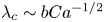 ${\lambda _c}\sim bC{a^{ - 1/2}}$, where b is the height of the Hele–Shaw cell. Presence of
 $Ca$ demonstrates that viscosity difference
 $\mathrm{\Delta }\eta $ promotes the instability as an increase of
 $\mathrm{\Delta }\eta $ decreases the instability wavelength, while surface tension
 $\gamma $ inhibits the instability as an increase of the
 $\gamma $ increases the instability wavelength. There exists a critical capillary number
 $C{a_c}$ which leads to the fingering instability with wavelength
 $\lambda $, i.e.
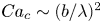 $C{a_c}\sim {(b/\lambda )^2}$. Pitts & Greiller (Reference Pitts and Greiller1961) studied coating of surfaces of counter-rotating half-submerged cylinders parallel to each other and observed formation of patterns at the film free surface with wavelength
 $\lambda $ proportional to
 ${(rb)^{1/2}}$. Here, r is the radius of the cylinders and b is the film thickness. Combination of these two scalings leads to a critical capillary number of the form
 $C{a_c} \sim b/r$ which may define the onset of viscous instability at an interface with radius r (Grillet et al. Reference Grillet, Lee and Shaqfeh1999). This is equivalent to stating that the height alterations formed at a curved free surface can be caused by the Saffman–Taylor instability. In our work, the Marangoni effect leads to shear in a thin film while the spreading creates a curved interface. The radius of curvature can be approximated as
 ${R_{in}}$, which is also the radius of the inner region (see figure 4c–e), i.e. the characteristic curvature length scale is of the same order of magnitude as the stream-wise length scale. We can conclude that the experimentally measured onset conditions leading to formation of the radially aligned patterns on Newtonian film (figure 4e) are caused by the Saffman–Taylor instability with the onset capillary number expressed as
 \begin{equation}C{a_c} \sim \frac{{{h_0}}}{{{R_{in}}}}.\end{equation}
The radially aligned rib-like patterns were also observed in viscoelastic liquids (figure 3a–d) but the wavenumbers were smaller than those observed in Newtonian liquids, even for similar film viscosities. Information about the rib-like patterns formed in the Boger 1 and Boger 2 liquids was added to the phase diagrams in figures 4(a) and 4(b) for reference. The mechanism driving this instability is likely different from the Saffman–Taylor instability as the fluid elastic properties play a significant role; the discussion presented in § 3.1 documented that the rib-like patterns were correlated with the contact line instability.
3.3. Spreading radius on viscoelastic film
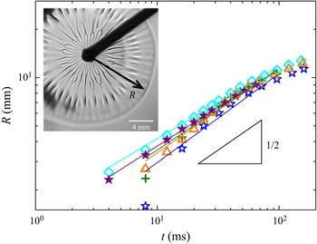
Time variations of the spreading radius R are illustrated in figure 5. Experiments were repeated several times for the same nominal conditions to illustrate reproducibility as well as to estimate the experimental errors. These results demonstrate that R increases proportionally to  ${t^n}$, with
 $n = 0.505 \pm 0.04$, which is close to 0.5, indicating that the spreading process results from an interplay between the Marangoni stress
 $S/R$ (the reservoir supply of surfactant is large enough to guarantee a constant
 $S$) and the viscous stress
 $\eta \dot{\gamma } = \eta (R/t)/{h_0}$ (Matar & Craster Reference Matar and Craster2009), with
 $\eta $ the viscosity of the film, and
 $\dot{\gamma }$ being the shear rate defined as ratio of the characteristic spreading velocity and the film thickness. The spreading parameter in this experiment was
 $S = {\gamma _B} - {\gamma _d} = 29.2\;\textrm{mN}\;{\textrm{m}^{ - 1}}$, t stands for characteristic time and
 ${h_0}$ is the fluid film thickness, and their combination leads to
 ${R^2} \sim {h_0}St/\eta$. This scaling law is also valid in spreading on a Newtonian film which suggests that the elastic effects do not play a significant role, at least during the observation time used in the experiments. This contrasts with the previous studies which demonstrated that elasticity was affecting system dynamics at short times such as observed in a falling film (Gaillard et al. Reference Gaillard, Roché, Lerouge, Gay, Lebon and Limat2019) as well as in the droplet spreading on a thick layer (Ma et al. Reference Ma, Zhong, He, Liu and Li2020). We shall discuss in the following subsections the interface shapes formed during spreading on both Newtonian and Boger liquid films. We shall use PTV to analyse the flow fields and to extract information about the film thickness. We shall also use the transmission-speckle method to extract information about the interface shape.
Temporal variations of the spreading radius R for thin films of Boger 2 fluid. Experiments were repeated five times to demonstrate their reproducibility. Each experimental dataset is identified using different symbols and colours.

3.4. Film height and flow field measurements
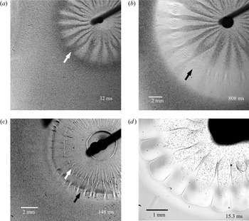
To study variations of film thickness caused by Marangoni spreading, we seeded a film with 10 μm diameter particles which provided a means for the qualitative determination of the film thickness distribution. A large particle density (1.6 × 10⁷ particles per cm3) was used for macroscopic transmission imaging (see figure 2a). The recorded images demonstrate the formation of the azimuthally alternating darker and lighter zones (see figure 6a,b and supplementary movie S2). The particles’ diameter is an order of magnitude smaller than the film thickness which means that the perceived larger density of the particles observed in the transmission experiment reflects the local film thickness; increase of darkness corresponds to an increase of film thickness. Comparison of images created using the seeded film with images produced with the un-seeded film show that the patterns in figure 6(a) overlap with the rib-like patterns in figure 3(a). This confirms that the rib-like patterns correspond to the local thickening of the film. The Marangoni ridge corresponds to the darkest colour in figure 6(a); it is identified using a white arrow. At approximately 800 ms, a severely thinned region, indicated by a black arrow in figure 6(b), is formed upstream of the ridge where particles are pinned to the surface. We estimate that the film thickness at this region was of the order of 10 μm, which is similar to the particle diameter. Finally, we note that the height distribution discussed above refers to the interface between the Boger film and the spreading droplet, as only the Boger film was seeded.
Droplet spreading on liquid films visualized using the light transmission method. Films were seeded with 10 μm particles. (a) Very initial (t = 32 ms) spreading on Boger 2 film with the initial thickness  ${h_0} = 60\;\mathrm{\mu }\textrm{m}$; gradations of grey correspond to regions of thicker (darker) and thinner (lighter) film; the white arrow identifies the position of the Marangoni ridge. (b) Same experiment as in panel (a) at the final stage of spreading (t = 808 ms) showing severely thinned regions with particles pinned to the surface identified using a black arrow. (c) Spreading on Newtonian PEG liquid film with a comparable viscosity and with the initial thickness
 ${h_0} = 60\;\mathrm{\mu }\textrm{m}$ showing uniform particle distribution in the azimuthal direction at a position indicated by the white arrow; the black arrow identifies the severely thinned region. (d) Spreading of a surfactant-laden droplet seeded with 10 μm particles on the Boger 2 film without particles. The particles’ distribution identifies spreading paths of the droplet.

Spreading on Newtonian films does not lead to observable changes of particle density (see figure 6c and supplementary movie S2). The radially aligned patterns are still visible due to the light refraction at the interface. This indicates that surface height variations, if any, are smaller than 10 μm (see figure 6c). We need to underline that smaller height variations may exist; however, they cannot be identified using the particle-seeded experiment. A shear flow should occur in the Newtonian film with particles near the solid boundary being retained due to friction. Hence, although both the Newtonian and the Boger films exhibit the formation of radially aligned patterns and rib-like structures at the film–droplet interface, the azimuthal height variations are much larger in the viscoelastic film. This conclusion is further confirmed by experiment with seeding removed from the film and added to the droplet; the particles’ trajectories indicate the existence of zones covered with the spreading droplet leaving other zones free of particles (figure 6d and supplementary movie S3). The particle-free zones have the same structure as the rib-like patterns displayed in figure 3(a). This confirms that the interface is thicker in the zones corresponding to the ribs, and the spreading liquid flows in the zones between the ribs.
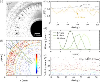
We return to the spreading experiment with particles seeded in the liquid films. For analysing the particle distribution, we begin with spreading on a Newtonian film; typical images are shown in figures 7(a) and 7(b). We wish to determine the azimuthal distribution of the number of particles left in the film after Marangoni spreading, and to deduce from it the film thickness. Before spreading, particles were nearly evenly distributed in the film;  ${\rho _0}$ denotes the initial particle average number density per unit of area determined by dividing the total number of particles seen in the initial images displayed in the supplementary movie S4 by the area of the viewing zone excluding the droplet deposition zone where particles were obstructed by the droplet. Analysis was carried out in the test region; a circular region bounded by two orange dashed lines shown in figure 7(b). This area was divided into 77 sub-regions in the azimuthal direction and the initial particle number density
 ${\rho _{t = 0}}(\theta )$ was determined in each sub-region; its average value was
 $1.05{\rho _0}$ and its variations with
 $\theta $ were minor, as illustrated by the grey line in figure 7(c). After the Marangoni ridge has passed through this region, e.g. at
 $t = 8.14\;\textrm{ms}$, the measured
 ${\rho _t}(\theta )/{\rho _0}$ exhibits irregular variations with the difference between the maximum and the minimum being less than 0.5; these variations do not exhibit periodicity in the azimuthal direction, as illustrated by the orange line in figure 7(c). However, the average density of particles left in the test region decreased since
 ${\rho _t}(\theta )/{\rho _0} < 1$ for most θ values with the average being
 ${\rho _t}(\theta )/{\rho _0} = 0.83$ (see orange dashed line in figure 7c). This means that the spreading process convected some of the liquid radially outwards leaving a layer of Newtonian film with an estimated thickness of
 $0.83{h_0}$. To the best of our knowledge, previous studies dealt only with determination of the droplet–air surface profile during a droplet spreading on the same fluid (Zhang et al. Reference Zhang, Matar and Craster2002; Afsar-Siddiqui et al. Reference Afsar-Siddiqui, Luckham and Matar2003b). The available literature does not report the state of the substrate film retained after the Marangoni spreading (Bacri et al. Reference Bacri, Debrégeas and Brochard-Wyart1996; Motaghian et al. Reference Motaghian, van Esbroeck, van der Linden and Habibi2022; Keiser et al. Reference Keiser, Bense, Colinet, Bico and Reyssat2017).
Particle tracking velocimetry (PTV) measurements for the Marangoni spreading on the Newtonian PEG fluid (see table 1) with the initial film thickness  ${h_0} = 59\;\mathrm{\mu }\textrm{m}$. (a) Picture taken at
 $t = 8.14\;\textrm{ms}$ from the beginning of spreading. (b) Particles identified from data in panel (a) with the colour and vector length indicating velocities of individual particles. (c) Azimuthal distributions of the normalized surface particle density
 ${\rho _t}(\theta )/{\rho _0}$ in the region bounded by the two dashed orange lines in panel (b) at times
 $t = 0$ and
 $t = 8.14\;\textrm{ms}$. (d) Radial distributions of the depth- and azimuthally averaged velocity in the region bounded by the two solid green lines in panel (b). (e) Azimuthal variations of the depth- and radially averaged particle velocities at the Marangoni ridge; colours of the dots indicate the velocities of individual particles and the red line indicates the depth- and radially averaged value.

We measured the velocity field during spreading to provide a quantitative explanation for the height variations of the interface between the film and the spreading droplet. The film was seeded with a smaller number of particles (particle density was 1.6 × 10⁶ particles cm−3) and individual particles were tracked under a microscope by PTV. A sequence of images was recorded during the spreading and positions of selected particles were identified in each image. Particles in two subsequent images were matched by the ‘nearest neighbour’ method which led to the determination of their trajectory and velocity. Supplementary movies S4 and S5 illustrate the particles’ motion in the Newtonian and Boger films, respectively. One concern is how accurately the position and motion of the particles reflects the motion of the fluid around it. It is known that particles close to the solid surface are subjected to electrostatic forces hindering diffusion and shear-induced rotation that induce biases to the velocity measurement (Li et al. Reference Li, D'eramo, Lee, Monti, Yonger, Tabeling, Chollet, Bresson and Tran2015). In this work, we do not attempt to obtain the velocity profile across the film but rather the depth-averaged velocity and its in-plane distribution. In this sense, the possible relative motion between the particles and the fluid can be neglected. In supplementary movie S4 and figure 7(b), the colour and the length of velocity vectors indicate the magnitude of the particle velocity. The radial velocity distribution in the test region bounded by two green solid lines (see figure 7b) is plotted in figure 7(d) at three time instances. This region was divided into 36 sub-regions along the radial direction, and the velocity at each sub-region was both depth and azimuthally averaged. The Marangoni ridge corresponds to the velocity peak; it is located between the two red solid lines shown in figure 7(b). The depth and radially averaged velocity in the ridge exhibit minor azimuthal variations, as illustrated in figure 7(e). This correlates well with the minor variations of the thickness of the film left after passing of the ridge (see figure 7c). These results suggest that the distributions of the depth-averaged velocity and the film height can be considered as being axisymmetric in the case of a Newtonian fluid. The radially aligned patterns observed by the light transmission method represent small perturbations at the film–droplet interface.
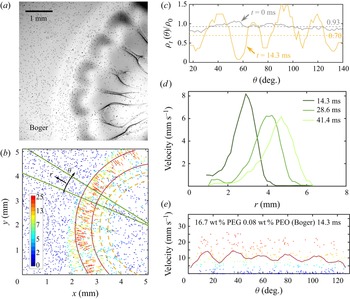
The analogical experiment with spreading on a Boger film seeded with particles demonstrated change in the response which can only be attributed to the viscoelastic effect (see supplementary movie S5). Many particles were observed in several radially aligned zones, whereas very few were observed in between, as illustrated by the image displayed in figure 8(a). The initial particle density  ${\rho _{t = 0}}(\theta )$ in the test region bounded by the two dashed orange lines was approximately
 $0.93{\rho _0}$, as illustrated by the grey line in figure 8(c). After the Marangoni ridge passed through this zone, i.e. at
 $t\; = 14.3\;\textrm{ms}$, the normalized particle density
 ${\rho _t}(\theta )/{\rho _0}$ showed large-amplitude azimuthal variations with the difference between the maximum and the minimum being approximately 1 and the maximum being larger than 1 (see orange line in figure 8c). This suggests the formation of a large-amplitude, regular film–droplet interface deformation with the film thickness higher than the initial thickness at some
 $\theta $ positions and lower at other
 $\theta $ positions. The average particle density retained in the test region was
 $0.7{\rho _0}$, as shown by the dashed orange line in figure 8(c). This means that the average film thickness in the test region after spreading was
 $0.7{h_0}$. The observed variations of the film height can be attributed to two effects. The first effect is the immobilization of particles which are too close to the solid surface, similar as in the Newtonian case. The second effect has its origins in the viscoelastic property of the Boger liquid. The viscoelastic instability was widely studied in the Taylor–Couette flows which produce curved streamlines and shear in the azimuthal direction (Shaqfeh Reference Shaqfeh1996). The radial velocity perturbation can be amplified by the elastic normal stress to produce modulations aligned in the azimuthal direction. Graham (Reference Graham2003) revealed theoretically that in the case of free curved interfaces, a ribbing instability of a viscoelastic film can be induced by the elastic normal stress which is in addition to the bulk elastic instability. In this work, the Marangoni spreading caused high-shear flow in the radial direction and led to formation of a curved film–droplet interface (figure 3a); this provided conditions for the onset of elastic instability and formation of the rib-like patterns at the film–droplet interface. The droplet spreading on top of the film had an uneven thickness whose form correlated with an instability at the droplet–film–air contact line which led to the formation of wide fingers in figure 3(a).
PTV measurements for the Marangoni spreading on the Boger 2 fluid with the initial film thickness  ${h_0} = 59.2\;\mathrm{\mu }\textrm{m}$. (a) Image recorded at
 $t = 14.3\;\textrm{ms}$ from the beginning of spreading. (b) Particles identified in the image displayed in panel (a) with their colours and vector lengths indicating the velocities of individual particles. (c) Azimuthal distributions of the normalized surface particle density
 ${\rho _t}(\theta )/{\rho _0}$ in the region bounded by the two dashed orange lines in panel (b) at times
 $t = 0$ and
 $t = 14.3\;\textrm{ms}$. (d) Radial distributions of the depth- and azimuthally averaged velocity in the region bounded by the two solid green lines in panel (b). (e) Azimuthal variations of the particle velocities at the Marangoni ridge; colours of the dots indicate velocities of individual particles and the red line indicates the depth- and radially averaged value.

The observed rib-like patterns (figure 3a) correlate well with the velocity field in the film. Figure 8(d) displays radial variations of the depth and azimuthally averaged velocity in the region delimitated by two solid green lines marked in figure 8(b) at three time instances during spreading; the velocity peaks in these plots identify locations of Marangoni ridge. Figure 8(e) displays azimuthal variations of the depth and radially averaged particle velocities in the zone around the ridge marked by two solid red lines in figure 8(b) at time  $t = 14.3\;\textrm{ms}$; the results demonstrate periodic variations of this velocity. It can be concluded that the Boger fluid in the high velocity zones of the ridge moves faster outwards leaving a thinner film in the inner region, while a thicker film is left in the low velocity zones leading to the formation of the rib-like patterns.
The above information, which was extracted using particles, provides a semi-quantitative description of the film thickness in the zone where the rib-like patterns were formed. The velocity distribution in the Marangoni ridge played a crucial role in determining the spatial distribution of these patterns. This conclusion is consistent with the results presented in figure 3(b) which demonstrated that the wavenumber of the rib-like patterns was similar to the wavenumber of the wide fingers at the film–droplet–air contact line.
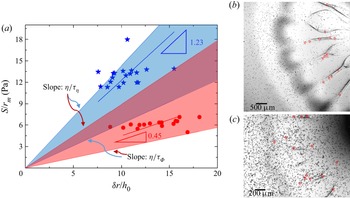
We shall now discuss the velocity field in the rib-like patterns. We observed that these patterns extended radially outwards during the spreading, and then retracted slightly inwards while the Marangoni ridge was still propagating outwards (see supplementary movie S5). This indicates that the elastic effects play a significant role in the ribs’ evolution. The velocity in the ribs is much smaller than the velocity in the Marangoni ridge. Particles which follow the rib retraction (see supplementary movie S5) are located near the film–droplet interface (see figure 9b,c). Particles that do not retract with the ribs are likely situated near the solid surface which restricts their movement and, thus, cannot represent the fluid motion near the film–droplet interface. Consider a particle which had an initial radial position  ${r_0}$. It moved out radially, reached a maximum radial position
 ${r_m}$ and then moved back radially following the rib retraction. If the fluid in the rib undergoes a shear deformation, then
 $\delta r = {r_m} - {r_0}$ is the displacement and
 $\delta r/{h_0}$ is the strain, where
 ${h_0}$ is the initial film thickness. The stress causing the deformation can be estimated as
 $S/{r_m}$ (radial surface tension gradient), where S is the spreading parameter defined in § 3.1. We measured
 ${r_0}$ and
 ${r_m}$ for several particles and plotted the corresponding strain and stress in figure 9(a). The slope of linear fitting of all the points for a Boger fluid, subject to the constraint that the line passes through the origin, defines a characteristic elastic shear modulus, which is
 $G = 1.23\;\textrm{Pa}$ for the Boger 1 fluid and
 $G = 0.45\;\textrm{Pa}$ for the Boger 2 fluid. These values can be compared with the shear moduli determined by rheological measurements of both fluids (Oswald Reference Oswald2009). The viscoelastic relaxation time obtained from the measurement of the first normal stress difference
 ${\tau _\phi }$ and viscosity
 ${\tau _\eta}$ reported in table 1 define a range of magnitudes of the shear moduli
 $G = [\eta /{\tau _\phi };\;\eta /{\tau _\eta }]\;\textrm{Pa}$ for both liquids. The PTV results overlap with the coloured area representing the range of G in figure 9(a), which shows that the slopes from PTV measurements agree with the shear moduli G from rheological measurements. This suggests that the ribs undergo elastic shear deformation in response to a surface-tension-gradient-caused Marangoni spreading. The relation between the spreading parameter S and the displacement field
 $\delta r$ can therefore be presented in the following form:
 \begin{equation}\frac{S}{{{r_m}}} \sim \frac{\eta }{\tau }\frac{{\delta r}}{{{h_0}}}.\end{equation}
Slopes of straight lines connecting the origin and each of the experimental points in figure 9(a) represent local elastic shear moduli. The PTV measurements reveal the existence of a range of such moduli for the Boger fluids, which agrees with data obtained from the rheological measurements.
Determination of the elastic shear moduli for the Boger fluids by the PTV method. (a) Variations of the surface tension gradient as a function of the strain in the zone characterized by the formation of the rib-like patterns. The blue colour corresponds to the Boger 1 fluid with the initial thickness  ${h_0} = 39.5\;\mathrm{\mu }\textrm{m}$ and the red colour to the Boger 2 fluid with the initial thickness
 ${h_0} = 59.2\;\mathrm{\mu }\textrm{m}$. The shear moduli are determined by the slopes (1.23 and 0.45) through linear curve fitting. Borders of the coloured areas are determined by the shear modulus
 $G = [\eta /{\tau _\phi };\;\eta /{\tau _\eta }]$ calculated from a rheological measurement (see table 1). (b) Particles in the rib-like structures in the Boger 2 fluid. (c) Image similar to panel (b) but for the Boger 1 fluid. The red dots in panels (b) and (c) identify particles used in panel (a). Their movement follows the extension and retraction of the ribs which demonstrates that they are located at the film–droplet interface and their motion reflects the shear-driven interface deformation.

3.5. Interface deformation analysis using the transmission-speckle method
In the previous subsection, the height of the Boger film was deduced from an analysis of the movement of particles with the particle surface density indicating the film thickness, at least semi-quantitatively. The thickness of the liquid film that remained after passing of the Marangoni ridge was determined. In this subsection, we analyse the shapes of the film–droplet and droplet–air interfaces.
We present this discussion in the context of spreading of a surfactant-laden droplet on top of the Boger 2 film with the initial thickness  ${h_0} = 93\;\mathrm{\mu }\textrm{m}$. An image of the deformed speckles at time
 $t = 1.7\;\sec $ is displayed in figure 2(d), i.e. when the spreading reached its final state. The zone subject to analysis forms a quarter-circle, identified by the red line in figure 2(d). Before getting into a detailed discussion, we wish to point out that the speckle method measures only the cumulative effect; if multiple interfaces are involved, as is the case in our experiment, it is unable by itself to separate the contributions from different interfaces. In our experiments, both liquids have nearly the same refractive indices, which means the contributions of the film–droplet interface to the overall refraction are small and extremely small in the case of a small interface deformation. In contrast, the refractive indices of the droplet and air are very different which means that this interface will bring in large contributions to the overall light refraction even if the interface deformation is small.
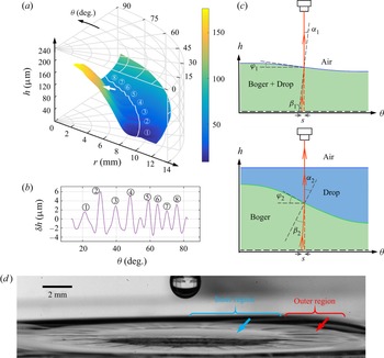
Let us assume that the contribution of the film–droplet interface to the light refraction is negligible and proceed on this basis with the analysis and interpretation of measurements. The measured height of the droplet–air interface is displayed in figure 10(a). The film thickness decreases radially outwards from the droplet deposition point forming a thin region and then starts to increase towards the ridge; these variations are in a qualitative agreement with the axisymmetric Marangoni spreading reported by Jensen & Grotberg (Reference Jensen and Grotberg1992). Azimuthal height variations with amplitude in the range of 6–10 μm can be seen in the thin region; detailed measurements were carried out along the white line shown in figure 10(a) with results displayed in figure 10(b). These variations correspond to the corrugation pattern formed at the droplet–air interface, which is visible in the outer region of the side-view of the spreading droplet displayed in figure 10(d). The same measurements also show height variations in the range of 2–4 μm in the inner region, as indicated by the white arrow in figure 10(a). Since these patterns were not observed in the side-view of the droplet–air interface in figure 10(d) (see the blue arrow), it can be concluded that they occurred at the film–droplet interface which was beneath the droplet–air interface. Let us restate arguments presented at the beginning of this subsection. In the case of very similar refractive indexes, the speckle virtual displacement is negligible if the film–droplet deformation is small. If the same interface has a large deformation with high slopes, then the speckle virtual displacement is large. This situation is sketched in figure 10(c); the upper sketch explains a simple refraction at the droplet–air interface with small slope and the lower sketch explains refraction at the film–droplet interface with large slope and a flat droplet–air interface. Both cases lead to the same speckle virtual displacement S. We can estimate that the inclination angle  ${\varphi _1}$ (see figure 10c) corresponding to the characteristic speckle virtual displacements (usually 0–3 pixels, i.e. 0–30.35 μm) is no more than 5° for the droplet–air refraction (upper figure 10c), whereas the inclination angle
 ${\varphi _2}$ is up to 40° for the film–droplet refraction (lower figure 10c). This suggests that the inner region is characterized by large height variations of the film–droplet interface. In summary, the droplet–air deformation dominates in the outer region while the film–droplet deformation dominates in the inner region.
Deformation of interfaces during droplet spreading on the Boger 2 film with the initial thickness  ${h_0} = 93\;\mathrm{\mu }\textrm{m}$ measured using the transmission-speckle method. (a) Shape of the droplet–air interface determined under the assumption that the deformation occurs only at this interface. The area used in the analysis is shown in figure 2(d). The white line (a circular line with radius of 9.2 mm and centred about the droplet deposition point) identifies locations of measurement points at the droplet–air interface in the outer region used in panel (b). The white arrow points to the apparent azimuthal height variations of the order of 2–4 μm at the droplet–air interface in the inner region which are due to the azimuthal deformations at the film–droplet interface. (b) Azimuthal height variations
 $\delta h$ along the white line in panel (a). Here,
 $\delta h = h - \bar{h}$, with
 $\bar{h}$ being the mean value of h. (c) Sketch of the interfacial deformation at the droplet-air interface (upper sketch) and at the Boger film–droplet interface with a flat droplet–air interface (lower sketch). Both cases lead to the same speckles’ virtual displacement S. The angles
 ${\alpha _1}$ and
 ${\alpha _2}$ are the refractive angles at the droplet–air interface and at the film–droplet interface, respectively,
 $\; {\beta _1}$ and
 ${\beta _2}$ are the incident angles, and
 ${\varphi _1}$ and
 ${\varphi _2}$ stand for the inclination angles of the deformed interfaces. (d) Side view of the droplet and the film at t = 1.7 s. The blue arrow points to the inner region where the droplet–air interface appears to be smooth and the red arrow points to the corrugation patterns at the droplet–air interface in the outer region.

The possible mixing between the Boger film and the surfactant-laden droplet can be driven only by diffusion. The time available for diffusion is determined by the characteristic time scale  ${t_s}$ of Marangoni spreading, which ranges from
 $0.01\;\textrm{s}$ to 0.1 s. The depth that diffusion can reach during that time can be estimated by considering water molecules diffusing normally into the Boger fluid with the characteristic length scale being
 ${l_D} \sim {(D{t_s})^{1/2}}$, where D stands for the diffusion coefficient which can be deduced from the Stokes–Einstein equation, i.e.
 $D \sim {k_B}T/(6{\rm \pi}\eta a)$, where
 ${k_B}T$ is the thermal energy,
 ${k_B}$ is the Boltzmann coefficient, T is the temperature,
 $\eta $ denotes the viscosity of the Boger film and a stands for the size of a water molecule. In our system,
 $D \sim 3.4 \times {10^{ - 11}}\;{\textrm{m}^2}\;{\textrm{s}^{ - 1}}$ and
 ${l_D}$ ranges from 0.6 μm to 1 μm for
 ${t_s}$ ranging from 0.01 s to 0.1 s; this
 ${l_D}$ is two orders of magnitude smaller than the thickness of the film. This means that the Boger liquid and the spreading droplet can be viewed as being immiscible during Marangoni spreading with a well-defined interface separating them. Both these liquids have the form of aqueous solutions with ultra-low surface tension which is 3–4 orders of magnitude smaller than the surface tension at the water–air interface (Atefi, Mann & Tavana Reference Atefi, Mann and Tavana2014); these conditions correspond to very large capillary numbers which means that the Marangoni spreading can produce steep azimuthal variations of the interface. If we assume that the deformation occurs only at the Boger film–droplet interface (lower figure 10c), calculations give the azimuthal height variations in the inner region to be approximately 100 μm. This assumption corresponds to an extreme case when the droplet–air interface deformation is negligible. Figure 10(d) shows that the droplet–air interface in the inner region is axisymmetric which means that the azimuthal variations at the film–droplet interface dominate the azimuthal deformation recorded by the speckles’ virtual displacement. The height variations of the film–droplet interface are comparable to the initial film thickness
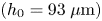 $({h_0} = 93\;\mathrm{\mu }\textrm{m)}$ in this experiment. This conclusion is a qualitative agreement with the particle surface density measurements (figure 8c) which showed the amplitude of azimuthal height variations to be of the order of the initial film thickness. Hence, we conclude that the Marangoni spreading induces deformation of both the Boger film–droplet and the droplet–air interface, but at different locations. The Boger film–droplet interface undergoes large deformations in the inner region forming rib-like patterns with height comparable to the initial film thickness. The droplet–air interface undergoes large deformations in the outer region, especially in the thinned part of this region during later stages of spreading, with the height of the corrugation patterns being of the order of 6–10 μm.
The current transmission-speckle method cannot accurately determine the interface shapes for arbitrary conditions when two interfaces are present; it can however provide useful information for special conditions such as those used in our experiment. It provides a qualitative information about the shape of the liquid film and it clearly documents the existence of the azimuthal variations of the Boger film–droplet interface, which occur beneath the droplet–air interface, and their existence was identified using a combination of the light transmission and transmission-speckle methods. A new technique using two different light wavelengths with different refractions at each interface and leading to different speckle virtual deformation fields amenable to individual analyses might resolve limitations of the current methodology when two interfaces are present (Tang, Dong & Liu Reference Tang, Dong and Liu2017).
4. Discussion
Studies of surfactant-laden droplets deposited and spreading on a more viscous Newtonian as well as viscoelastic films are important for understanding the dynamics of drug-loaded droplets’ landing on mucus in the airways and spreading on it. Elucidation of the role played by Marangoni-driven shear flow, the viscosity contrast and the viscoelasticity of liquids is essential for the development of proper drug delivery strategies.
Marangoni spreading represents an extremely complex configuration for the study of the contact line instability, including the determination of its onset conditions and understanding of its wavelength selection mechanism. The spreading process is complex as the spreading velocity cannot be controlled as in other configurations, e.g. blade-coating or roll-plate coating, with this velocity resulting from an interplay between the surface tension and the film thickness; the capillary number  $Ca$ cannot be imposed but results from the process dynamics. The spreading velocity decreases with time without being affected by fluid elasticity and the spreading radius R increases with time as
 ${t^{1/2}}$ (see figure 5).
We have constructed a phase diagram in the 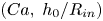 $(Ca,\; {h_0}/{R_{in}})$-plane (see figure 4) which determines the critical capillary number
 $C{a_c}$ for the onset of instability leading to the formation of radially aligned patterns on Newtonian films. Results obtained for two viscoelastic fluids (Boger 1 and Boger 2) are consistent with the Newtonian results; however, the effect of elasticity on
 $C{a_c}$ remains to be established. Studies available in the literature have demonstrated the importance of elasticity in the onset of the contact line instability. Deblais et al. (Reference Deblais, Harich, Colin and Kellay2015), in their blade-coating experiment, defined a range of
 $Ca$ in which the receding contact line becomes unstable and forms cusp-like patterns; this range appears to be similar for both Newtonian and viscoelastic fluids, but the effect of elasticity on the onset conditions was not reported. In an experiment involving the roll-plate shear flow between eccentric cylinders (Grillet et al. Reference Grillet, Lee and Shaqfeh1999), the fluid at the receding contact line exhibits fingering patterns above a critical
 $C{a_c}$ for a fixed normalized film thickness; the value of this
 $C{a_c}$ decreases in viscoelastic fluids. This suggests that the elasticity plays a destabilizing role at the receding contact line instability beyond a simple amplification of processes leading to the formation of cusp-like patterns. These patterns are characterized by the formation of a stationary contact line which surrounds the air fingers. Bauman et al. (Reference Bauman, Sullivan and Middleman1982) studied the ribbing instability in the roll-plate coating experiment with the roll being half submerged in a liquid with its axis parallel to the free surface and plate placed vertically next to the roll. They demonstrated that the viscoelastic effect produced ribbing in an extensional flow on the free surface. The same viscoelastic effect caused a fingering/cusping instability at a receding contact line (Grillet et al. Reference Grillet, Lee and Shaqfeh1999; Deblais et al. Reference Deblais, Harich, Colin and Kellay2015). In addition, the rib-like patterns are reminiscent of cracks formed on gel surfaces caused by Marangoni spreading (Spandagos et al. Reference Spandagos, Goudoulas, Luckham and Matar2012a,Reference Spandagos, Goudoulas, Luckham and Matarb), in which the critical condition for cracks to occur is that the shear stress overcomes the storage modulus of the gel
 $G^{\prime}$, i.e.
 $S/\Delta w > G^{\prime}$, where S is the spreading parameter defined in § 3.1 and
 $\Delta w$ is the change in the width of the crack. In our experiments, the azimuthal distance between the rib-like patterns is of the order of 100 μm, so that
 $S/\Delta w$ is of the order of 100 Pa, which is much larger than the elastic moduli
 $G = 1.23\;\textrm{Pa}$ and 0.45 Pa of our Boger fluids (see figure 9a). This shows that the Marangoni stress in our experiments is large enough to ‘crack’ the Boger film and to form the rib-like patterns. The behaviour of a viscoelastic liquid film under strong shear fits between the Newtonian film on which only weak interface perturbations are observed and of a pure elastic surface on which cracks are observed. The formation of rib-like patterns on viscoelastic film and the azimuthal wavelength selection are worth a further study.
Deblais et al. (Reference Deblais, Harich, Colin and Kellay2015) in their blade-coating experiment reported that the instability wavelength depended on the shearing velocity as  $\lambda \sim {V^{3/4}}$, which meant that
 $\lambda $ increased with
 $Ca$. Grillet et al. (Reference Grillet, Lee and Shaqfeh1999), however, reported that in their roll-plate coating experiment, the wavenumber k increased with the
 $Ca$ for both the Newtonian and viscoelastic fluids, with the elasticity modifying the wavenumber dependence on
 $Ca$. Graham (Reference Graham2003) explained how hoop stresses at curved interfaces generate a ribbing instability and gave the instability onset condition in the absence of gravity in the form
 $(1 - \beta )CaK\mathrm{\Sigma }/Wi > {k^2}h_0^2$, where
 $\beta$ stands for the solvent contribution to viscosity, K is the dimensionless surface curvature, Σ is the dimensionless normal stress difference,
 ${W_i}$ stands for the Weissenberg number, k denotes the wavenumber and
 ${h_0}$ stands for the initial film thickness. This shows that the ribbing instability favours small wavenumbers. An increase of
 $Ca$ destabilizes smaller wavelengths but, according to Graham (Reference Graham2003), the most unstable wavelength is never smaller than the film thickness. This finding is consistent with the results of our experiment. One can identify approximately 30 rib-like patterns in the image displayed in figure 3(b). Since these patterns are formed at the very beginning of the spreading, when the spreading radius is approximately 1 mm, the resulting wavelength is
 $\lambda \approx 200\;\mathrm{\mu }\textrm{m}$, as the initial thickness is
 ${h_0} = 85\;\mathrm{\mu }\textrm{m}$. Graham (Reference Graham2003) suggested that the fastest growing wavelengths for viscoelastic and Newtonian fluids are defined by
 $k{h_0} \approx 2$. In our experiment with a Boger fluid,
 $k{h_0} = 2{\rm \pi}{h_0}/\lambda \approx 2.7$. The growth rate of the unstable modes on a viscoelastic film is much larger than that on a Newtonian film according to Graham (Reference Graham2003), which is consistent with our observations which show that the heights of the rib-like patterns are comparable with the initial film thickness. However, we observed that in the case of Newtonian films, the number of radially aligned patterns was approximately twice the number of rib-like patterns on viscoelastic films with comparable viscosity; we suspect that these patterns result from the growth of several unstable modes with small but similar growth rates.
5. Summary
We have carried out experimental investigations of Marangoni spreading of a surfactant-laden droplet on thin films of Newtonian liquids with viscosity much larger than the droplet viscosity, as well as on viscoelastic liquids. The known phenomena, such as a strongly deformed interface and a severely thinned region upstream from the Marangoni ridge, were observed in agreement with the results available in the literature. In particular, the formation of radially aligned patterns was observed for both types of films in the inner region upstream from the Marangoni ridge, with their wavenumbers being much smaller for viscoelastic films than for Newtonian films despite comparable viscosities of both liquids. This indicates that this effect was induced by the liquid viscoelasticity. We used Newtonian fluids with different viscosities to study the critical condition for the onset of surface perturbations at the film–droplet interface. We found that a critical capillary number  $C{a_c}$ describes the onset of the interface deformation, which suggests that the radially aligned patterns result from the Saffman–Taylor instability at the film–droplet interface. The effect of the viscoelasticity on the critical
 $C{a_c}$ requires further study to establish the effect of elasticity numbers (Grillet et al. Reference Grillet, Lee and Shaqfeh1999). Changes of the film thickness resulting from Marangoni spreading were quantified by observing the movement of particles seeded in the film. The rib-like patterns exhibiting large variations in the azimuthal direction were observed at the Boger film–droplet interface. No similar azimuthal thickness variations were observed on Newtonian films. The azimuthal thickness variation of the viscoelastic film was confirmed using the transmission-speckle method, which indicated large height variations at the Boger film–droplet interface in the inner region, corresponding to the rib-like patterns. A PTV analysis showed azimuthal variations of the spreading velocity in (or near) the Marangoni ridge for Boger films, which demonstrated that the instability originated at the film–droplet–air contact line. The rib-like patterns determine the extent of the low-velocity zone near the contact line. These observations demonstrated the role of viscoelasticity in amplifying the receding contact line instability of the Boger film and in the formation of the rib-like patterns. Analysis of the flow field in the interior of these patterns suggests that the shear stress generated by the Marangoni spreading leads to an elastic shear deformation within the ribs.
The experiments reported in the paper provide a database which might inspire theoretical and computational analyses of viscoelastic effects in thin film Marangoni spreading. Additional work is required to understand the mechanism of wavelength selection in the observed instabilities. The knowledge of Marangoni spreading on viscous films with either Newtonian or viscoelastic properties is relevant to the inhaled drug delivery process. This work should contribute to a better understanding of aerosolized droplets landing and spreading on airways.
Supplementary movies
Supplementary movies are available at https://doi.org/10.1017/jfm.2023.108.
Acknowledgements
We acknowledge G. Hu, X. Wang and G. Chen for the helpful discussion, and Q. Liu, Q. Tian and K. Luo for their generous support of equipment.
Funding
This work is supported by NSFC Grant Nos. 12072033, 11802023 and 11972084.
Declaration of interests
The authors report no conflict of interest.