



1. Introduction
Aerodynamic noise from airfoils has been a topic of great significance over the past decades in various engineering applications, such as aircraft, wind turbines and aero-engines. Contrary to the inflow-turbulence interaction noise, the airfoil self-noise is generated in the absence of unsteady incoming turbulence and normally defines the lower bound of the airfoil noise (Wright Reference Wright1976). At low-to-moderate Reynolds numbers, the boundary layer on the airfoil surface is more likely to separate under adverse pressure gradients, leading to sound spectra comprising both tonal and broadband noise components (Brooks, Pope & Marcolini Reference Brooks, Pope and Marcolini1989).
Although considerable studies have reported on the tonal noise from airfoils, the underlying mechanism is still controversial. The earliest systematic study on the tonal noise of airfoils was conducted by Paterson et al. (Reference Paterson, Vogt, Fink and Munch1973). They experimentally investigated the tonal noise from a NACA0012 airfoil at different angles of attack (AoAs) in a wind tunnel, and studied Reynolds numbers range from 450 000 to 2 200 000. It was observed that the frequency of the tonal noise did not increase linearly with the incoming velocity. Instead, the frequency of the tonal noise jumped at critical Reynold numbers, resulting in a ‘ladder-type’ structure in the frequency–velocity spectrum of the tonal noise. Subsequently, Tam (Reference Tam1974) attributed the ‘ladder-type’ structure to the acoustic feedback loop (AFL) mechanism. They proposed that the large-scale unstable waves generated at the trailing edge (TE) were amplified as they propagated downstream, inducing pronounced transverse vibrations in the wake. These vibrations generated acoustic waves that propagated upstream, forcing the airfoil TE boundary layer to oscillate and establish an AFL. This AFL model was modified by Fink (Reference Fink1975), Longhouse (Reference Longhouse1977), Nash, Lowson & McAlpine (Reference Nash, Lowson and McAlpine1999) and Chong & Joseph (Reference Chong and Joseph2009), who suggested that the AFL occurred between the receiving point upstream of the TE and the TE. However, the location of the receiving point within the boundary layer remains a subject of debate. Arbey & Bataille (Reference Arbey and Bataille1983) indicated that the location of the maximum velocity of the boundary layer was the location of the receiving point, while the experimental study conducted on a NACA 0012 airfoil by Chong & Joseph (Reference Chong and Joseph2009) revealed that the initial point of the boundary-layer instability was probably the receiving point. Arcondoulis et al. (Reference Arcondoulis, Doolan, Zander, Brooks and Liu2019) suggested that the receiving point of the AFL model was located at the flow-separation point based on the wind-tunnel experiment on a NACA 0012 airfoil.
In addition, the types of the boundary-layer instability waves in the AFL model are also controversial. Chong & Joseph (Reference Chong and Joseph2009) proved that the ‘ladder-type’ structure of the airfoil tonal noise at different Reynolds numbers was due to the lag between the Tollmien–Schlichting (T–S) wave scattered from the TE of the airfoil and the feedback acoustic waves generated by the AFL, as demonstrated by tests on the NACA0012 airfoil. Pröbsting et al. (Reference Pröbsting, Serpieri and Scarano2014) and Pröbsting & Yarusevych (Reference Pröbsting and Yarusevych2015) conducted a series of particle image velocimetry (PIV) measurements on a NACA 0012 airfoil to investigate the mechanism of the tonal noise and the regions of tonal noise generation at different Reynolds numbers. It was found that at small AoAs, the tonal noise was related to the flow interactions from both sides of the airfoil. Pröbsting et al. (Reference Pröbsting, Serpieri and Scarano2014) further emphasised the importance of the laminar separation bubble (LSB) in the AFL, which acted as an amplifier of the instability waves within the boundary layer. Yakhina et al. (Reference Yakhina, Roger, Moreau, Nguyen and Golubev2020) also conducted wind-tunnel experiments on a symmetric NACA-0012 airfoil and a cambered SD7003 airfoil. It is shown that the presence of a LSB is essential for tonal noise, provided that the LSB is sufficiently close to the TE. Subsequently, Yang et al. (Reference Yang, Pröbsting, Li, Liu and Li2022) decomposed the flow fields over a NACA0012 airfoil at different Reynolds numbers employing the proper orthogonal decomposition (POD) technique. It turned out that the sideband tones in the noise spectrum of the airfoil were related to two different modulation interactions in the source region of the TE. Atassi (Reference Atassi1984) showed that the AFL associated with tonal noise was maintained via Kelvin–Helmholtz (K–H) instability waves, as the laminar separation occurred on the airfoil surface. Tam (Reference Tam1974) conducted an extended study on the tonal noise from a NACA 0012 airfoil using direct numerical simulations and proposed that the amplitude of the T–S instability wave was not sufficient to produce significant acoustic radiation through TE scattering. More recently, Sanjose et al. (Reference Sanjose, Towne, Jaiswal, Moreau, Lele and Mann2019) and Jaiswal et al. (Reference Jaiswal, Pasco, Yakhina and Moreau2022) further confirmed the existence of K–H instability waves in the AFL for the airfoil tonal noise both experimentally and numerically.
At low-to-moderate Reynolds number, another major constituent of airfoil self-noise is the broadband noise. Compared with the tonal noise, broadband noise encompasses a wider range of types and characteristics. In general, the broadband self-noise of the airfoil mainly arises from the random pressure fluctuations caused by the interaction between the multiscale vortices within the boundary layer and the TE. Therefore, the characteristics of the airfoil broadband self-noise are associated with the boundary-layer properties. At higher Reynolds numbers, the boundary-layer transition point shifts toward the TE, resulting in the presence of a turbulent boundary layer over most of the airfoil surface (Winslow et al. Reference Winslow, Otsuka, Govindarajan and Chopra2018). The turbulence-boundary-layer-TE noise (TBL-TE) is then produced by the interaction between the turbulent boundary layer and the airfoil TE (Brooks et al. Reference Brooks, Pope and Marcolini1989). A detailed review of the generation mechanism, the prediction model, as well as the control methods of the TBL-TE noise was presented in the review paper by Lee et al. (Reference Lee, Ayton, Bertagnolio, Moreau, Chong and Joseph2021). As flow separation persists along the airfoil surface without transition or reattachment prior to the TE, broadband self-noise can also be generated through the interaction of large-scale coherent structures in the separated boundary layer with the TE. Brooks et al. (Reference Brooks, Pope and Marcolini1989) categorised the broadband self-noise under such conditions as separation-stall noise. Compared with the TBL-TE noise, the separation-stall noise exhibits a greater low-frequency increase, exceeding 10 dB (Brooks et al. Reference Brooks, Pope and Marcolini1989), which has received relatively limited attention until now. The characteristics of the separation-stall noise are found to vary with the extent of flow separation on the airfoil surface. Under deep stall conditions, the boundary layer separates across the entire airfoil surface. The consequent increase in broadband far-field noise across a wide frequency spectrum is characterised as stall noise. At lower Reynolds numbers and lower AoAs, the laminar boundary-layer separation point may be delayed until the TE, preventing the separated boundary layer reattaching to the airfoil surface. Consequently, the broadband noise induced by flow separation intensifies within the low-frequency regime, forming a distinctive broadband hump in the far-field noise spectra. Such spectral features have been previously reported in the works of Moreau, Roger & Christophe (Reference Moreau, Roger and Christophe2009) and Lacagnina et al. (Reference Lacagnina2019). Moreau et al. (Reference Moreau, Roger and Christophe2009) investigated the acoustic performance of the NACA0012 airfoil at light stall and deep stall, and developed an analytical model to predict the separation-stall noise based on the Curle analogy. It was demonstrated that the flow-separation noise exhibits pronounced low-frequency components and dipole-like source characteristics. Moreover, distinct tones were observed in its spectrum, which were believed to be attributed to the instability of the shear layer and the shedding of large-scale vortices. Lacagnina et al. (Reference Lacagnina2019) further investigated the characteristics of the far-field noise on the NACA 65(12)-10 airfoil at various stall regimes, and established the connection between the surface pressure fluctuations and the flow motions within the separated boundary layer. Despite the relatively comprehensive understandings gained from previous studies regarding the characteristics and generation mechanisms of flow-separation noise, it is still challenging to achieve effective control of the broadband separation noise, owing to the stochastic nature of turbulent fluctuations.
Over the past few decades, the wavy leading edge (WLE) has attracted considerable attention as a passive flow-control approach for airfoils. The initial research interest in WLE was motivated by its potential to improve the aerodynamic performance of airfoils (Johari et al. Reference Johari, Henoch, Custodio and Levshin2007; Fish, Howle & Murray Reference Fish, Howle and Murray2008). A significant amount of work has been undertaken experimentally and numerically to demonstrate the ability of the WLE to delay the stall (Miklosovic et al. Reference Miklosovic, Murray, Howle and Fish2004; Fish et al. Reference Fish, Weber, Murray and Howle2011) and increase the lift of the airfoils (Favier, Pinelli & Piomelli Reference Favier, Pinelli and Piomelli2012; Rostamzadeh et al. Reference Rostamzadeh, Kelso, Dally and Hansen2013; Chong et al. Reference Chong, Vathylakis, McEwen, Kemsley, Muhammad and Siddiqi2015). It has been well established that the improved aerodynamic performance of WLE airfoils is attributed to a pair of counter-rotating streamwise vortices generated behind the WLE (Hansen et al. Reference Hansen, Rostamzadeh, Kelso and Dally2016). These vortices promote momentum transfer of the boundary layer, thereby delaying the flow separation and improving the aerodynamic performance. Owing to the modulation of the boundary layer by these streamwise vortices, WLE is found to effectively reduce both the tonal and broadband components of the airfoil’s self-noise (Wang et al. Reference Wang, Zhao, Lu, Song and Bennett2019).
For the tonal noise of the airfoils, Hansen, Kelso & Doolan (Reference Hansen, Kelso and Doolan2010) found that the WLE is able to eliminate the discrete tones and the surrounding broadband hump in the far-field noise from a NACA0021 airfoil through the wind-tunnel experiments at a Reynolds number of 12 000. They claimed that the noise-reduction mechanism is strongly related to the influence of the streamwise vortices on the stability of the boundary layer, yet the specific mechanism underlying this influence was not clarified in detail. Chong et al. (Reference Chong, Vathylakis, McEwen, Kemsley, Muhammad and Siddiqi2015) conducted experimental studies on the aeroacoustic performance of a NACA65(12)-10 airfoil with serrated leading edges (LEs). It was reported that the streamwise vortices induced by an optimised serrated LE could suppress the separation bubble near the TE, thereby significantly reducing the tonal noise. Chong et al. (Reference Chong, Biedermann, Koster and Hasheminejad2018) investigated the effectiveness of the WLE with different geometrical parameters in suppressing the airfoil self-noise by wind-tunnel measurements based on the NACA 65(12)-10 airfoil. It was found that the WLE with the largest magnitude and the smallest wavelength reduced the airfoil tonal noise most significantly. They also reported that the streamwise vortices generated by the WLE were effective in suppressing the LSB at the TE, thus disturbing the AFL responsible for the generation of the tonal noise. Later, Chen et al. (Reference Chen, Qiao, Duan and Wei2021) performed a series of experiments on a NACA 0012 airfoil to investigate the effect of the WLE on the airfoil tonal noise at different AoAs and Reynolds numbers. Consistent with Chong et al. (Reference Chong, Biedermann, Koster and Hasheminejad2018), they suggested that the WLE with the shortest wavelength and largest amplitude yielded the most significant noise reduction. More recently, Chen et al. (Reference Chen, Wang, Xing, Wang and Qiao2023) performed large eddy simulations (LES) to further investigate the mechanism of the WLE on the tonal noise reduction. It turned out that the WLE eliminated the LSB at the airfoil TE, resulting in a significant reduction of the pressure fluctuations and their spanwise coherence near the TE. While many studies have confirmed the effectiveness of the WLE in reducing tonal noise and have proposed explanations for its underlying mechanism, the generation mechanism of tonal noise in straight leading-edge airfoils is still controversial. As a result, previous investigations into the WLE’s noise-reduction mechanism have not clearly addressed this issue, and the conclusions remain inconsistent. Accordingly, one of the primary objectives of this study is to elucidate the generation mechanism of tonal noise in the straight leading-edge airfoil and to provide a more detailed understanding of the influences of the WLE-induced flow motions on the tonal noise generation.
Regarding the noise-reduction effect of the WLE on the broadband separation noise, Lacagnina et al. (Reference Lacagnina, Hasheminejad, Paruchuri, Joseph, Chong and Stalnov2017) presented an experimental investigation on a NACA-65 airfoil, and they noted that WLE can reduce the separation noise in the low-frequency range at small and negative AoAs. Subsequently, Lacagnina et al. (Reference Lacagnina, Paruchuri, Berk, Joseph, Hasheminejad, Stalnov, Chong and Ganapathisubramani2018) further examined the influence of the WLE on the broadband separation noise through experiments and PIV measurements. The results indicate that, while WLE airfoils may trigger more severe flow separation, this effect can significantly reduce the correlation between the wall pressure fluctuations and the far-field noise. Although previous studies have shown that the WLE can significantly suppress separation noise, the physical mechanism by which it influences the separation noise generated by the modified separation structure remains unclear.
This paper aims to elucidate the noise-reduction mechanism of the WLE on the self-noise from a cambered NACA 65(12)-10 airfoil at a Reynolds number of 100 000. The primary objectives of this paper are outlined as follows:
-
(i) Clarify the tonal noise generation mechanism of the baseline airfoil at low Reynolds numbers.
-
(ii) Investigate the effect of the WLE on the reduction of the tonal noise and the broadband separation noise in the low-to-mid frequency range.
-
(iii) Elucidate the underlying mechanisms of the WLE airfoils in suppressing both the tonal and the broadband separation noise by modifying the flow motions within the boundary layer.
The airfoil self-noise is measured in an anechoic wind tunnel using microphone arrays. Flow details closely relevant to the self-noise generation are obtained from both the PIV measurements and the wall-resolved LES, including the boundary-layer characteristics and the evolution of the streamwise vortices. The paper is organised as follows. Section 2 describes the experimental set-ups and the numerical methods. Detailed analysis on the flow characteristics is presented in § 3. The underlying mechanisms of the noise reduction are discussed from both the tonal and broadband aspects in § 4. Finally, some conclusions are summarised in § 5.
Geometrical parameters of the WLE airfoil.

2. Experimental set-up and numerical methods
2.1. Geometries of the airfoil
The cambered NACA 65(12)-10 airfoil is chosen as the baseline airfoil in this work, with a chord length
 $c_0=150\ \textrm{mm}$
. This asymmetric airfoil, commonly employed in turbomachinery, features a high camber design that delays the separation of the laminar boundary layer, thereby improving the aerodynamic performance. The geometry of the WLE airfoil and its geometrical parameters are illustrated in figure 1. For the WLE airfoil, the chord length
 $c$
along the spanwise direction follows a sine function characterised by the wavelength
 $\lambda$
and the amplitude
 $h$
. The profile
 $(x_{\textit{w}},y_{\textit{w}})$
of the WLE airfoil at the spanwise position
 $z$
is described as
 \begin{equation} \left \{ \begin{array}{l} x_{\textit{w}}=\left \{ \begin{array}{l} x_{\textrm{s}}-\Delta c\left ( \frac {x_{\textrm{s}}-x_c}{x_c} \right ) ,x_{\textrm{s}}\lt x_c,\\ x_{\textrm{s}},x_{\textrm{s}}\geqslant x_c,\\ \end{array} \right .\\ y_{\textit{w}}=y_{\textrm{s}},\\ \end{array} \right . \end{equation}
where
 $x_c$
is the coordinate at the maximum thickness of the baseline airfoil with the profile coordinates
 $(x_{\textrm{s}},y_{\textrm{s}})$
, and
 $\Delta c=c-c_0$
. In this study, the parameters of the WLE are inspired by the geometric characteristics of the leading-edge tubercles observed on humpback whale flippers. Based on the measurements reported by Fish & Battle (Reference Fish and Battle1995), the parameters of the WLE are set to
 $h/c_0=0.12$
and
 $\lambda /c_0 = 0.5$
. Symmetric airfoils designed with these parameters have been demonstrated to be effective for enhancing the aerodynamic performance at moderate Reynolds numbers (Cai et al. Reference Cai, Zhou, Liu, Zuo, Zhang and Li2022). As shown in § 4, a WLE airfoil configured with these parameters also exhibits effective suppression of far-field self-noise, thus providing a representative case for investigating the noise-reduction mechanisms of the WLE. The TE of the airfoils is designed to be flat, with a bluntness approximately 0.3 % of the chord length. Both the baseline and the WLE airfoil utilised in the experiments are fabricated using the 3D printing technique with the photosensitive resin. Additional surface treatments are applied to prevent the premature transition of the laminar boundary layer due to high surface roughness. Furthermore, the surfaces of the airfoils are painted with light-absorbing pigments to prevent the reflected light from contaminating the PIV measurements. It needs to be noted that the spans of the airfoils used in the acoustic and PIV measurements are
 $400\ $
and
 $500\ \textrm{mm}$
, respectively, due to the different directions of the airfoil installation.
2.2. Experimental set-up and instrumentations
2.2.1. Far-field noise
The far-field noise measurements are conducted in an anechoic wind tunnel, as shown in figure 2. The maximum jet speed of this wind tunnel is
 $\textrm{80 m s}^{-1}$
, while in this study the jet speed is set at
 $\textrm{10 m s}^{-1}$
with a chord-based Reynolds number
 ${Re_c=100\, 000}$
. Furthermore, the turbulence intensity in the free stream is less than
 $0.2\,\%$
, and the size of the nozzle is
 $500\ \textrm{mm}\times 400\ \textrm{mm}$
. The lowest cutoff frequency of the acoustic chamber is 100
 $\textrm{Hz}$
, decided by the shape of wedges on the chamber walls. Two side plates are flush mounted to the nozzle exit to eliminate the end effect of the airfoil. The airfoils used for the acoustic test are screwed vertically to the centre of the side plates, ensuring that the airfoils are not offset from the jet core. The LE of the airfoil is approximately
 $\textrm{500}\ \textrm{mm}$
downstream of the nozzle exit. Moreover, the AoA of the airfoil is kept as
 $0^\circ$
during the experimental trials.
Experimental set-up for the acoustic measurements. (a) Photo of the anechoic wind tunnel, (b) the top view of the experimental set-up for the acoustic measurements.

A circular microphone array is employed to measure the far-field noise from the airfoil, which consists of 12 half-inch microphones (GRAS 46AE). These microphones are located at a constant radial distance of
 $\textrm{1.5 m}$
from the centre of the airfoil. As depicted in figure 2, the microphones are symmetrically positioned on both sides of the nozzle exit, with an angular separation of
 $15^\circ$
between the adjacent microphones. To minimise the effect of the side plates on the airfoil noise, the height of the microphones are adjusted carefully to align with the middle span of the airfoil. The acoustic pressure signals are acquired over a duration of 30 s for each airfoil, utilising a sampling frequency of 100
 $\textrm{kHz}$
. In this study, both the sound pressure level (SPL) and the sound power level (PWL) spectra are employed to illustrate the noise-reduction performance of the WLE with respect to the baseline airfoil. Here,
 \begin{equation} \textrm{SPL} ( f ) =10\log _{10}\left ( \hat {P} ( f ) /p_{\textit{ref}}^{2} \right ), \end{equation}
where
 $\hat {P}(f)$
refers to the power spectral density (PSD) of the sound pressure, and
 $p_{\textit{ref}}=20\times 10^{-6}\,\textrm{Pa}$
is the reference sound pressure. The PSD spectra of the sound pressure are estimated using Welch’s method with a 40 960-point-sized hamming window and
 $50\,\%$
overlap. The PWL spectrum defined based on the PSD of the sound pressure is
 \begin{equation} \textrm{PWL}\left ( f \right ) =10\log _{10}\left \{ \left ( \frac {sr}{\rho a_0W_{\textit{ref}}} \right ) \left \{ \sum _{i=1}^N \left(\frac {\hat {P}(\theta _i,f)+\hat {P}(\theta _{i+1},f)}{2}\right)\Delta \theta \right \} \right \}, \end{equation}
where
 $a_0$
is the speed of sound,
 $s$
is the spanwise length of the airfoil,
 $r$
refers to the distance between the microphones and the centre of the airfoil,
 $\hat {P}(\theta _i,f)$
is the amplitude of the sound pressure PSD measured at the microphone with the angle of
 $\theta _i$
,
 $\Delta \theta$
is defined as the angle between two adjacent microphones and
 $W_{\textit{ref} }=10^{-12} \ \textrm{W}$
denotes the reference sound power.
2.2.2. Planar PIV measurement
To investigate the effect of the WLE on the flow structures and validate the LES simulations, planar PIV measurements are conducted on both the WLE and the baseline airfoils. The experimental apparatuses and a sketch of the set-up are demonstrated in figure 3. Different from the acoustical measurements, these airfoils are fixed horizontally to facilitate the laser installation. A smoke machine that produces solid particles is placed in front of the wind-tunnel compressor to generate homogeneous particles. An ILA.PIV.sCMOS camera equipped with a Canon EF 85 mm lens is utilised to acquire images, and the field of view is set as
 $365 \ \textrm{mm} \times 310 \ \textrm{mm}$
as shown in figure 3. A dual pulsed laser is used as the light source, and the pulse duration is set to
 $70\ \mu \textrm{s}$
. The laser emerges from the light guiding arm, positioned 1.5 m above the airfoil with a
 $90^\circ$
incidence angle. Besides, an additional convex lens and a mirror are placed beneath the airfoils to replenish lights under the airfoil. The velocity field on the mid-span plane is measured for the baseline airfoil, while both the peak and valley planes are measured for the WLE airfoil. A sequence of 1200 images are acquired for each case at a sampling frequency of
 $15\ \textrm{Hz}$
with a digital imaging resolution of
 $7\ \textrm{pixel/mm}$
. These images are processed using the Multiple-pass interrogation scheme, and a total of three passes are achieved. The window size is
 $16\times 16 \ \textrm{pixels}$
with an overlap ratio of
 $50\,\%$
. Overall, the effective spatial resolution of the PIV measurements is approximately
 $0.43 \ \textrm{mm}$
.
Experimental set-up for the PIV measurements. (a) Photo of the PIV measurement system, (b) the sketch of the experimental set-up for the PIV measurements.

2.3. Numerical method
2.3.1. Method of the flow-field simulation
In addition to the experimental measurements described above, wall-resolved LES simulations are also implemented in this paper to elucidate the underlying noise-reduction mechanism of the WLE airfoil. The simulations are employed to capture supplementary flow details to the PIV measurements. The velocity of the incoming flow is 10 m s−1, the same with that in the measurements, corresponding to a chord-based Reynolds number
 ${Re_c=100\, 000}$
. Since all experiments and simulations are conducted at low Mach number
 ${Ma} \leqslant 0.3$
, the incompressible Navier–Stokes (N–S) equations are solved in this study. The filtered incompressible N–S equations are
 \begin{align} \frac {\partial \tilde {u}_i}{\partial x_i} & =0.\end{align}
 \begin{align} \frac {\partial \tilde {u}_i}{\partial t}+\frac {\partial \tilde {u}_i\tilde {u}_j}{\partial x_j} & =-\frac {1}{\rho _0}\frac {\partial \tilde {p}}{\partial x_i}+\nu \left ( \frac {\partial ^2\tilde {u}_i}{\partial x_{j}^{2}}+\frac {\partial ^2\tilde {u}_j}{\partial x_{i}^{2}} \right ) -\frac {\partial \tau _{ij}}{\partial x_j},\end{align}
where
 $\tilde {u}_i$
and
 $\tilde {u}_j$
represent the filtered velocity components in the Cartesian coordinates
 $x_i$
and
 $x_j$
;
 $\nu$
is the kinematic viscosity;
 $\rho _0$
and
 $\tilde {p}$
represent the density and the modified pressure, respectively;
 $\tau _{ij}$
is the subgrid-scale stress tensor computed based on the eddy-viscosity approximation
 \begin{equation} \tau _{ij}=\frac {1}{3}\tau _{kk}\delta _{ij}-2\nu _{sgs}\tilde {S}_{ij}, \end{equation}
where
 $\tilde {S}_{ij}=({1}/{2}) (({\partial \tilde {u}_i}/{\partial x_j})+({\partial \tilde {u}_j}/{\partial x_i}) )$
is the resolved-scale strain rate tensor; and
 $\nu _{sgs}$
is the subgrid-scale viscosity computed with the wall adapting local eddy-viscosity (WALE) model
 \begin{equation} \nu _{sgs}=\left ( C_w\varDelta \right ) ^2\frac {\left ( S_{ij}^{d}S_{ij}^{d} \right ) ^{3/2}}{\left ( \tilde {S}_{ij}\tilde {S}_{ij} \right ) ^{5/2}+\left ( S_{ij}^{d}S_{ij}^{d} \right ) ^{5/4}}, \end{equation}
where
 $\varDelta$
is the subgrid characteristic length scale;
 $C_w$
is the WALE constant, which is set as 0.325 in this study;
 $S_{ij}^{d}=({1}/{2}) ( \tilde {g}_{ij}^{2}+\tilde {g}_{ji}^{2} ) -({1}/{3})\delta _{ij}\tilde {g}_{kk}^{2}$
is the square of the velocity gradient tensor;
 $\tilde {g}_{ij}$
is defined as
 \begin{equation} \tilde {g}_{ij}=\frac {\partial \tilde {u}_i}{\partial x_j}. \end{equation}
The LES simulations are performed using the open-source computational fluid dynamics software OpenFOAM, while the Gauss linear differencing scheme is adopted for the spatial discretisation, and the backward differencing scheme is utilised for the temporal discretisation. Furthermore, the coupled velocity and pressure are solved using the pressure-implicit with splitting of operators algorithm. The time step of the LES is set as
 $10^{-5}\,\textrm{s}$
to ensure that the maximum Courant number over the entire computational domain is less than 1.0. All simulations are initially run for 10 flow-through times (based on the free-stream velocity and the streamwise size of the overall computational domain) to reach a statistically converged steady state before starting the data acquisitions. The statistical data used for the analysis are then collected over another 10 flow-through times.
A sketch of the computational domain.

2.3.2. Computational domain and mesh
A schematic diagram of the computational domain is shown in figure 4. The origin of the coordinate system is positioned at the TE of the airfoil, aligned with the mid-span. The dimensions of the computational domain are
 $10c_0$
in the streamwise (
 $x$
) direction,
 $6c_0$
in the cross-flow (
 $y$
) direction. To enhance the computational efficiency, the spanwise (
 $z$
) width of the airfoil is much smaller than that used in the experiments. For the baseline airfoil and the WLE airfoil, the spanwise dimensions are
 $0.24c_0$
and
 $2\lambda$
, respectively. The no-slip wall boundary condition is imposed on the surface of the airfoil. The velocity inlet boundary condition is assigned to the inlet, with a corresponding chord-based Reynolds number
 $Re_c=100\,000$
. The outlet is imposed with the pressure outlet boundary condition. The periodic boundary condition is applied to the spanwise direction.
The computational domain is discretised into fully structured cells. Grid independence investigations on the baseline airfoil are conducted to evaluate the most suitable grid resolution for the LES simulation. The mean lift and drag coefficients (
 $\overline {C_l},\,\overline {C_d}$
) and their root-mean-square (r.m.s.) values (
 $C_{l, {\textit{rms}}},\,C_{d, {\textit{rms}}}$
) are calculated to evaluate the effect of the mesh resolution on the LES results. Details of the mesh independence studies are summarised in table 1. It is shown that the differences in
 $\overline {C_l}$
and
 $\overline {C_d}$
between case 2 and case 3 are negligible. In terms of balancing the accuracy and the computational efficiency, the mesh resolution of case 2 is more practical for the LES simulations in this work. In case 2, there are 682 nodes along the profile on the
 $x{-}y$
plane and 80 evenly distributed nodes along the spanwise direction, leading to a total number of
 $6.47\times 10^6$
cells. For the WLE airfoil, the total number of cells is
 $11.0\times 10^6$
, with 572 nodes and 113 nodes along the airfoil profile and the span, respectively. As shown in figure 5, except for the region close to the LE, where larger velocity gradients exist, the wall-unit grid spacings of case 2 in table 1 are
 $\Delta y^+ \leqslant 1$
,
 $\Delta x^+ \leqslant 100$
and
 $\Delta z^+ \leqslant 40$
, which meet the mesh requirement of the wall-resolved LES.
Details of the grid independence studies for the baseline airfoil.

Wall-unit grid spacings of the baseline airfoil.

2.3.3. Validations of the numerical method
To gain confidence in the LES simulations in this work, the numerical results of the baseline airfoil and the WLE airfoil are evaluated comprehensively. The lift and drag coefficients are consistent with the experimental measurements on NACA 65(12)-10 airfoils conducted by Kim et al. (Reference Kim2022) (
 $\overline {C_l}=0.50,\,\overline {C_d}=0.05$
), as the flow condition in the study of Kim et al. (Reference Kim2022) without a grid upstream of the airfoil is comparable to the present study. Moreover, the distribution of the averaged pressure coefficient
 $C_p=(\bar {p}-p_0)/(0.5\rho _0U_{\infty }^{2})$
along the baseline airfoil is compared with the
 $C_p$
value obtained from the xFoil software using the panel method, experimental results from Lacagnina et al. (Reference Lacagnina2021) and the numerical results from Tong et al. (Reference Tong2018). Reasonable agreements are observed in the pressure coefficient
 $C_p$
of the baseline airfoil compared with the other results, as shown in figure 6, implying the feasibility of the LES simulations in this study.
Comparisons of the time-averaged pressure coefficients for the baseline airfoil.

Besides the comparisons with the existing literature, the averaged streamwise velocity profiles at different locations along the suction surface of the baseline and the WLE airfoil calculated by the LES are also compared with those obtained from the PIV measurements in figure 7. As validated by the PIV results, the mean streamwise velocity profiles within the boundary layer are accurately predicted by the LES employed in this study. Furthermore, the turbulent kinetic energy (TKE) distributions within the wakes of both the baseline and WLE airfoils are compared with the PIV measurements in figure 8 to further assess the capability of the numerical method in predicting the unsteady flow characteristics of the airfoils. As shown in figure 8, the double peak of the TKE profile is well captured in the present LES for both the baseline and the WLE airfoil downstream of the TE. This feature arises from the different velocity gradients in the boundary layers on the airfoil’s suction and pressure surfaces (Liu et al. Reference Liu, Kamliya Jawahar, Azarpeyvand and Theunissen2017). In addition, as shown in figure 8(b), the secondary peak in the TKE profile in the wake of the WLE airfoil around
 $y/c_0= -0.15$
is also accurately captured by the LES. This peak is associated with the unique vortex system originated from the valley on the pressure side of the WLE airfoil, which will be discussed in detail in § 3.2.
Comparisons of the mean streamwise velocity (
 $\overline {u_x}$
) profile on the suction surface of the airfoils. (a) Mid-plane of the baseline airfoil, (b) valley plane of the WLE airfoil.

Comparisons of the TKE (
 $k$
) profile in the wake of the airfoils. (a) Mid-plane of the baseline airfoil, (b) valley of the WLE airfoil.

Given that the instability waves generated within the boundary layer on the airfoil surface play a crucial role in the tonal noise generation, the capability of the employed LES in resolving the dominant instability waves in the separated boundary layer (i.e. the K–H instability waves, which will be discussed in § 4) is further validated. Two probes are placed along the shear line (defined as the trace of the mean shear stress profile maximum points, where
 $\partial ( -\overline {u_x^{\prime }u_y^{\prime }} ) /\partial y=0$
) to sample the streamwise velocity fluctuations
 $u^\prime _x$
. The streamwise positions of these probes are
 $x/c_0=-0.1$
and
 $x/c_0 =-0.15$
, respectively. The corresponding PSD spectra are obtained via the Welch method, as shown in figure 9(a). Both spectra exhibit a prominent peak at a Strouhal number of
 ${St}=fc_0/u_{\infty }=3$
. The corresponding non-dimensional frequency based on the boundary-layer-edge velocity
 $U_s$
and the momentum thickness
 $\theta _s$
at the separation point
 $St_s = f\theta _s/u_s = 0.005$
falls within the range of 0.005–0.013, which is the typical range of the inviscid K–H instability waves (Yang & Voke Reference Yang and Voke2001). Furthermore, the PSD spectra of the wall pressure fluctuations
 $p^\prime$
at two stations,
 $x/c_0=-0.1$
and
 $x/c_0 =-0.15$
, on the suction surface of the baseline airfoil are shown in figure 9(b), along with the PWL of the experimentally measured far-field noise from the baseline airfoil for reference. The peak frequencies in the PSD spectra of the wall pressure fluctuations coincide with both the dominant tone in the far-field noise and the frequency of the K–H instability waves. These results indicate that the present LES accurately predicts the characteristics of the instability waves within the boundary layer.
Overall, the reasonable agreement between the LES predictions and the experimental measurements demonstrates that the LES approach employed in this study can reliably predict both the mean and instantaneous characteristics of the flow field and capture the critical fluid dynamic mechanism directly responsible for the TE tonal noise generation.
Validation of the frequency of the K–H instability wave in the separated boundary layer of the baseline airfoil from the numerical simulation. (a) The PSD of the streamwise velocity fluctuations
 $u^\prime _x$
, (b) the PSD of wall pressure fluctuations
 $p^\prime$
.

3. Effect of the WLE on the flow-field characteristics
Wall pressure fluctuations on the airfoil are one of the predominant sources of airfoil self-noise. In many cases, the far-field noise can be accurately predicted using the classical flat-plate theory, provided that statistical data of the wall pressure fluctuations near the TE are available. As suggested by Lee et al. (Reference Lee, Ayton, Bertagnolio, Moreau, Chong and Joseph2021), the spectral characteristics and the intensity of the wall pressure fluctuations are attributed to the statistical properties of the pressure fluctuation, the turbulence intensity and the vortex structure scales within the separated boundary layer. Therefore, in view of the close relation between the airfoil self-noise and the dynamic characteristics of the flow field, the time-averaged properties of the flow field and the spatio-temporal evolution of the coherent structures around the airfoil are analysed based on the experimental and numerical results. Considering the notable disparities in the boundary layer on the suction and the pressure sides, separate examinations of the flow fields on both sides of the baseline and the WLE airfoils are provided in the subsequent sections.
3.1. Flow characteristics above the suction surface
The instantaneous vortices above the suction surface of the baseline airfoil and the WLE airfoil are visualised in figure 10, based on the isosurface of the
 $Q$
-criterion at
 $Q_n=5$
, where
 $Q$
is the second invariant of the velocity-gradient tensor. The isosurface is coloured by the averaged streamwise velocity, and
 $Q_n$
is the normalised Q-criterion
 \begin{equation} Q_n=\frac {Q}{\left ( u_{\infty }/c_0 \right ) ^2} \end{equation}
As shown in figure 10(a), quasi-two-dimensional spanwise vortex rollers are observed in the separated boundary layer on the suction surface of the baseline airfoil, which are associated with the K–H instability. These vortex rollers merge and break up as they convect toward the TE, stretching into three-dimensional vortex clusters near the TE.
These spanwise vortices induced by the K–H instabilities play an important role in the generation of tonal noise. Moreover, as shown in figure 10(b), on the suction side of the WLE airfoil, a rolled-up boundary layer is observed at the initial separation region near the valley. These rolled-up vortices do not extend spanwise and break up rapidly toward the TE, transitioning into turbulence. As a result, the boundary layer on the suction surface near the TE of the WLE airfoil is dominated by the smaller scaled vortices and thereby enhances momentum mixing within the near-wall boundary layer. The reduction in spanwise vortex coherence induced by the WLE prevents the vortices from maintaining sufficient strength as they approach the TE, thereby suppressing periodic vortex shedding and the TE scattering. This process effectively disrupts the mechanism responsible for tonal noise generation, which will be addressed in detail below.
Isosurface of the instantaneous flow structures on the suction side at
 $Q_n=5$
, coloured by the mean streamwise velocity (LES results). (a) Baseline airfoil and (b) WLE airfoil.

Figure 11 shows the time-averaged streamwise velocity and the Reynolds shear stress
 $\overline {u_x^\prime u_y^\prime }/u_\infty ^2$
at the mid-span of the baseline airfoil along with those at the peak and valley of the WLE airfoil obtained from the PIV experiments. The separation and transition positions of the boundary layer over the suction surface are marked by the triangles shown in figure 11, and the transition locations are determined by the criterion
 $\overline {u_x^\prime u_y^\prime }/u_\infty ^2=0.001$
proposed by Ol et al. (Reference Ol, McCauliffe, Hanff, Scholz and Kähler2005). As shown in figure 11(a), the boundary layer of the baseline airfoil on the upper surface is separated at approximately
 $x/c_0=-0.33$
. The streamlines reveal a primary recirculation bubble, accompanied by a secondary recirculation region upstream it. Such recirculation bubbles near the TE are suggested to be the necessary condition for the generation of the tonal noise, as these structures are able to amplify the hydrodynamic waves within the separated boundary layer (Wu, Sandberg & Moreau Reference Wu, Sandberg and Moreau2021). As shown in figure 11(b), the region of the intense momentum mixing is observed downstream of the TE of the baseline airfoil, as evidenced by the increased Reynolds shear stress. Consequently, the separated boundary layer is unable to reenergize upstream of the TE to reattach to the airfoil surface.
Contours of the time-averaged velocity (left column) and the Reynolds shear stress (right column) at different spanwise locations. (a–b) Mid-span of the baseline airfoil, (c–d) peak of the WLE airfoil, (e–f) valley of the WLE airfoil. The white dash-dotted line denotes the locations where
 $\bar {u}_x =0$
(experimental results). Here, S, T denote the estimated locations of separation and transition, respectively.

As shown in figures 11(c) and 11(e), the laminar boundary layer on the suction surface of the WLE airfoil separates initially at
 $x/c_0=-0.4$
at the valley while the separation at the peak is delayed to
 $x/c_0=-0.3$
. Variations in boundary-layer separation over the WLE airfoil have also been reported in previous studies (Hansen, Kelso & Dally Reference Hansen, Kelso and Dally2011; Skillen et al. Reference Skillen, Revell, Pinelli, Piomelli and Favier2015), and these variations have been associated with the enhanced aerodynamic performance of the WLE airfoil. In addition, the recirculation bubbles are also observed at the TE of the WLE airfoil, while the secondary recirculation region vanishes. The white dash-dotted line shown in figure 11(e), denoting the locations where
 $\overline {u_x} =0$
, is observed to adhere to the wall at
 $x/c_0=-0.2$
and enters the flow fields at
 $x/c_0=-0.14$
at the valley of the WLE airfoil. This suggests that the boundary layer at the valley of the WLE airfoil exhibits a short reattachment after the initial separation. Nevertheless, due to the fact that the Reynolds shear stress upstream of the reattachment point is relatively small, it implies that the reattachment observed at the valley of the WLE airfoil is not attributable to the reenergisation induced by the boundary-layer transition. As shown in figures 11(d) and 11(f), compared with the baseline airfoil, the Reynolds shear stress grows rapidly upstream of the TE above the suction surface of the WLE airfoil. At the valley of the WLE airfoil, the region of the high Reynolds shear stress is brought closer to the airfoil surface, suggesting that the smaller-scaled vortices at the valley induce an intense momentum transfer within the separated boundary layer. Notably, an additional region of high Reynolds shear stress exists beneath the pressure surface of the WLE airfoil. This is attributed to the counter-rotating vortex induced by the WLE on the airfoil’s pressure surface, which will be discussed in detail in § 3.2.
To analyse the effect of the WLE on the characteristics of the boundary layer, figure 12 shows the coefficients of the skin-friction (
 $C_f$
), pressure (
 $C_p$
) and r.m.s. wall pressure fluctuations (
 $C_{\overline {p^\prime }}$
) along the suction surfaces of the WLE and the baseline airfoils calculated based on the LES simulation. Consistent with the PIV results shown in figure 11(e), the short reattachment at the valley of the WLE airfoil is verified by the negative
 $C_f$
at
 $ -0.24\leqslant x/c_0\leqslant -0.12$
shown in figure 12(a). Moreover, the separation of the laminar boundary layer leads to a pressure plateau with almost constant
 $C_p$
in figure 12(b). According to the characteristics of the surface pressure distribution of the LSB described by O’meara & Mueller (Reference O’Meara and Mueller1987), the start and the end of the pressure plateau of
 $C_p$
indicate the positions of the separation and the transition. A stronger adverse pressure gradient is observed upstream of the separation point at the valley of the WLE airfoil, which is responsible for the advanced boundary-layer separation. Furthermore, it is shown in figure 12(c) that rapid growth of
 $C_{\overline {p^\prime }}$
starts from
 $x/c_0=-0.28$
and
 $x/c_0=-0.2$
for the valley of the WLE airfoil and the baseline airfoil, respectively, followed by the transition of the shear layer.
Coefficients on the suction surface of the baseline and the WLE airfoils calculated based on the LES data at different spanwise locations (LES results). (a) Skin-friction coefficients, (b) pressure coefficients and (c) r.m.s. wall pressure fluctuations.

Figure 13 illustrates the contour of the pressure coefficients on the suction surface of the WLE airfoil and the flow topology depicted by the wall skin-friction lines. Downstream of the LE of the WLE airfoil, the skin-friction lines are deflected by the WLE and converge towards the valley. As a result, the flow converging towards the valley is accelerated due to the increased local AoA, leading to an enhanced suction peak at the valley. Furthermore, the suction peak of the WLE airfoil at the valley is advanced upstream compared with the peak plane, resulting the variation in the pressure along the spanwise direction. The spanwise pressure gradient, as suggested by Gad-el Hak (Reference Gad-el Hak2000), is the predominant mechanism to drive the generation of the streamwise vorticity above the airfoil surface. According to the spanwise momentum equation at the wall with the facts that there is no flow injected from the wall and the viscosity is constant
 \begin{equation} \left . \frac {\partial p}{\partial z} \right |_{y=0}=\left . \mu \frac {\partial ^2w}{\partial y^2} \right |_{y=0}, \end{equation}
where the spanwise pressure gradient
 $\partial p/ \partial z$
is proportional to the flux of the streamwise vorticity.
Contour of
 $C_p$
and the skin-friction lines on the suction surface of the WLE airfoil (LES results).

The dimensionless mean streamwise vorticity
 $\overline {\omega _x}c_0/u_\infty$
at different chordwise positions is depicted in figure 14. As shown in figure 14(a), the vorticity above the suction surface of the WLE airfoil is dominated by a pair of counter-rotating primary vortices and the wall vortices beneath them. The high-inertia boundary-layer fluid is transported away from the valley by the primary vortices, leading to a rapid dissipation of the momentum. As depicted in figure 14(b), a new pair of vortices is generated near the wall due to the reversed direction of the spanwise pressure gradient downstream
 $x/c_0=-0.6$
. As shown in figures 14(b) and 14(c), the primary vortices are lifted away from the valley and dissipated gradually by the viscous effects as they convect downstream, forming a canopy of vorticity above the separation zone which corresponds to the previous findings (Hansen et al. Reference Hansen, Rostamzadeh, Kelso and Dally2016). The high-momentum fluid from the outer boundary layer is transported into the separated boundary layer by the counter-rotating primary vortices, re-energising the separated boundary layer and leading to its reattachment within the range of
 $ -0.3\leqslant x/c_0\leqslant -0.2$
. As shown in figure 14(d), the direction of the wall vortices on the suction surface reverses downstream
 $x/c_0=-0.4$
. The dominant vortices generate a concentrated upwash flow at the valley location, leading to boundary-layer re-separation. Downstream at
 $x/c_0=-0.2$
as shown in figures 14(e) and 14(f), the streamwise vorticities exhibit almost homogeneous distributions due to the turbulent transportation after the transition of the boundary layer.
The streamwise vortices induced by the WLE are considered to be responsible for the enhanced aerodynamic performance (Hansen et al. Reference Hansen, Kelso and Dally2011; Cai et al. Reference Cai, Zuo, Maeda, Kamada, Li, Shimamoto and Liu2017) and reduction of the tonal noise of the airfoil (Hansen et al. Reference Hansen, Kelso and Doolan2010; Chen et al. Reference Chen, Wang, Xing, Wang and Qiao2023). Hansen et al. (Reference Hansen, Rostamzadeh, Kelso and Dally2016) observed similar counter-rotating streamwise vortices in their experiments and simulations on the airfoil NACA0012. In their study, the streamwise vortices were intensified by the continuous injection of boundary-layer vorticity and lifted after the formation of a pair of foci on the suction surface, maintaining considerable strength up to the TE. This behaviour contributed to a noticeable improvement in the aerodynamic performance of the WLE airfoil. In contrast, our simulations show that, without the presence of surface foci as shown in figure 13, the wall-bounded streamwise vorticity can still be lifted away from the surface. Nevertheless, the absence of boundary-layer vorticity injection results in a rapid dissipation of the streamwise vortices. In this case, the WLE airfoil used in the present study remains effective in reducing the tonal noise as well as the broadband separation noise in the low-to-mid-frequency range. These findings suggest that the underlying noise-reduction mechanism may be attributed to the modulation of the boundary layer after the separation by the streamwise vortices.
Dimensionless mean streamwise vorticity
 $\omega _x c_0/u_\infty$
over the suction surface of the WLE airfoil at various chordwise positions (LES results). Panels show (a)
 $x/c_0=-0.6$
, (b)
 $x/c_0=-0.5$
, (c)
 $x/c_0=-0.4$
, (d)
 $x/c_0=-0.3$
, (e)
 $x/c_0=-0.2$
, (f)
 $x/c_0=-0.1$
.

Overall, the spanwise variation of the profile of the WLE airfoil alters the local AoA, leading to the acceleration of the flow at the valley, thereby inducing the spanwise pressure gradients on the suction surface of WLE airfoil. This spanwise pressure gradient acts as the source of the streamwise wall vorticity flux, as denoted by the vorticity transport equation (3.2). Within the WLE boundary layer, the momentum transfer caused by streamwise vortices substantially modifies boundary-layer characteristics. On the one hand, it alters the separation points and boundary-layer thickness along different spanwise positions on the suction surface of the WLE airfoil, thereby changing the local K–H instability frequencies and weakening the spanwise coherence of the rolled-up boundary layer, which supports the conclusions of Hansen et al. (Reference Hansen, Kelso and Doolan2010). On the other hand, the vortex-induced enhanced turbulent mixing rapidly fragments the large-scale vortices into smaller three-dimensional structures, further suppressing the growth of the K–H instability waves. This phenomenon disrupts the mechanism responsible for tonal noise generation at its source, which will be verified by the experimental results in § 4.2. It should be also noted that the WLE does not significantly suppress the TE separation bubble, suggesting that the WLE-induced tonal noise-reduction mechanism proposed by Chen et al. (Reference Chen, Wang, Xing, Wang and Qiao2023) may not be applicable to the present case.
3.2. Flow characteristics beneath the pressure surface
The instantaneous vortices at
 $Q_n=5$
, beneath the pressure surfaces of both the baseline and the WLE airfoils, are illustrated in figure 15. As shown in figure 15(a), the boundary layer of the baseline airfoil on the pressure surface transitions to turbulence near the LE, while the characteristic K–H instability-type vortices are observed. For the WLE airfoil, as shown in figure 15(b), a series of hairpin vortices originating from the valley is observed at the pressure surface. These hairpin vortices are lifted away from the airfoil surface as they evolve downstream, accompanied by the merging and breakdown. The region of high Reynolds shear stress beneath the pressure surface of the WLE airfoil shown in figure 11(f) is attributed to the momentum mixing induced by these hairpin vortices. Particularly, the morphology and the evolution of these hairpin vortices exhibit a striking resemblance to the vortex system downstream a micro-ramp at the critical ramp-height-based Reynolds number
 ${Re_h}$
(Ye, Schrijer & Scarano Reference Ye, Schrijer and Scarano2018).
Isosurface of the instantaneous flow structures on the pressure side at
 $Q_n=5$
, coloured by the mean streamwise velocity (LES results). (a) Baseline airfoil and (b) WLE airfoil.

Figure 15. Long description
Panel A: A three-dimensional visualization of the instantaneous flow structures on the pressure side of a baseline airfoil. The structures are colored by the mean streamwise velocity, with a color scale ranging from blue to red. The K-H instability is labeled, showing turbulent flow patterns. Panel B: A similar three-dimensional visualization for a WLE airfoil. The hairpin vortices are labeled, indicating different flow structures compared to the baseline airfoil. The color scale is also from blue to red, representing the mean streamwise velocity.
Due to the limitations of the PIV measurements on the region under the pressure surface of the airfoil, the analysis of the flow characteristics on the pressure side mainly relies on the LES simulations. Figure 16 presents the distributions of
 $C_f$
,
 $C_p$
and
 $C_{\overline {p^\prime }}$
at various spanwise locations along the pressure surfaces of the WLE and the baseline airfoils. The skin-friction coefficient
 $C_f$
of the baseline airfoil, as shown in figure 16(a), indicates the boundary-layer separation and the subsequent reattachment near the LE of the pressure surface, leading to the formation of a spanwise LSB. The existence of the spanwise LSB near the LE of the pressure surface of the NACA 65(12)-10 airfoil is also reported in the experimental study of Gruber (Reference Gruber2012). Furthermore, the rapid increase of
 $C_{\overline {p^\prime }}$
observed at
 $x/c_0 = -0.9$
for the baseline airfoil in figure 16(c) provides the evidence of the transition of the separated boundary layer. The turbulent boundary layer on the pressure surface of the baseline airfoil interacts with the TE, leading to broadband components of the far-field noise. For the WLE airfoil, the spanwise length of the short LSB on the pressure surface is reduced compared with the baseline airfoil, as evidenced by the absence of the positive value of
 $C_f$
near the LE of the WLE airfoil at the peak shown in figure 16(a). As shown in figure 16(c), the r.m.s. pressure coefficients at the peak show less variation compared with that at the valley, indicating that the boundary layer remains laminar at the peak. In fact, the boundary layer along the peak of the WLE airfoil exhibits a delayed separation, occurring around
 $x/c_0=-0.4$
, with reattachment to the wall observed near
 $x/c_0=-0.1$
, as denoted by the
 $C_f$
in figure 16(a).
Coefficients on the pressure surface of the WLE and the baseline airfoils calculated based on the LES data at different spanwise locations (LES results). (a) Skin-friction coefficients, (b) pressure coefficients and (c) r.m.s. wall pressure fluctuations.

Complex three-dimensional flow structures are developed on the pressure side of the WLE airfoil due to the leading-edge geometry of the WLE airfoil. Therefore, the topologies of the skin-friction lines on the pressure surface of the WLE airfoil are analysed in this paper to reveal the characteristics of the three-dimensional separated flow. Figure 17 shows the contour of the pressure coefficient
 $C_p$
on the pressure surface of the WLE airfoil, superimposed by the skin-friction lines. The critical points (saddle, node and focus points) formed by the pattern of the skin-friction lines are classified by the identification criteria proposed by Délery (Reference Délery2001).
As shown in figure 17, the skin-friction lines at the LE near the valley of the WLE airfoil emanate from the saddle point S1 and converge at the node points N1, N2, generating a short separation line. Downstream of the separation line, the node point N3 together with the saddle points S2 and S3 show the typical characteristics of the attachment line, where the separated flow reattaches to the surface. These separation and attachment lines delineate the imprint of the short LSB near the LE on the pressure side of the WLE airfoil. Particularly, the short LSB functions similarly to a micro-ramp as described by Ye et al. (Reference Ye, Schrijer and Scarano2018), as the formation and the growth of the hairpin vortices at the valley of the WLE airfoil shown in figure 15(b) are attributed to the K–H instability within the shear layer over the short LSB. Furthermore, the estimated height-based Reynolds number
 ${Re_h}$
based on the height of the short LSB is 582, falling in to the supercritical range of
 ${Re_h}$
. At the supercritical
 ${Re_h}$
, the K–H instability in the boundary layer undergoes transient growth, giving rise to the formation of the hairpin vortices and subsequently inducing the transition. In addition, on both sides of the short LSB, the skin-friction lines converge into the attachment lines indicated by the blue dash-dotted lines shown in figure 17. The attachment lines terminate on the saddle points S6 and S7 near the TE of the WLE airfoil, which indicate the boundaries of the turbulence flow originated from the valley. Two saddle points, S4 and S5, located at
 $x/c_0=-0.375$
are also found in figure 17. Furthermore, two separation lines emanate from the saddle points S4 and S5. The skin-friction lines converge towards the separation lines and eventually leave the wall at the foci points F1 and F2. As a result, a pair of tornado-like vortices are generated, emanating perpendicularly from the wall at F1 and F2 and subsequently deflected by the free stream, forming a pair of counter-rotating vortices downstream. The global separation lines indicate the location of the boundary-layer separation on the pressure surface of the WLE airfoil, where an evident increase of
 $C_{\overline {p^\prime }}$
is observed in figure 16(c).
Contour of the
 $C_p$
and the skin-friction lines on the pressure surface of the WLE airfoil. The blue dot-dashed lines indicate the location of the attachment lines (LES results).

Figure 17. Long description
Panel A: A heat map showing the contour of skin-friction lines on the pressure surface of the WLE airfoil. The x-axis is labeled x/c0 and ranges from -1.0 to 0. The y-axis is labeled z/λ and ranges from 0 to 0.5. The color scale at the top ranges from -0.6 to 0.6, indicating the value of Cp. The blue dot-dashed lines indicate the location of the attachment lines. Several regions are labeled with identifiers such as N1, N2, N3, S1, S2, S3, S4, S5, S6, S7, F1, and F2. The heat map shows areas of varying skin-friction values, with distinct patterns and regions of high and low friction.
Similar to the suction surface, spanwise pressure gradients are also found along the pressure surface of the WLE airfoil, as shown in figure 16(b). Consequently, it is not surprising to observe the counter-rotating vortices driven by the spanwise pressure gradients beneath the pressure surface of the WLE airfoil. The streamwise vorticity at different chordwise positions is depicted in figure 18. In fact, the streamwise vortices beneath the pressure surface of the WLE airfoil can be classified into two different types: the streamwise vortices driven by the spanwise pressure gradient (region A in figure 18
a) and the streamwise vortices induced by the short LSB at the valley (region B in figure 18
a). As shown in figures 18(a) and 18(b), a pair of counter-rotating wall vortices with a pair of primary vortices beneath them are formed, driven by the spanwise pressure gradient as discussed in § 3.1. At the valley of the WLE airfoil, a new pair of counter-rotating vortices (CP1) emanates from the edge of the LSB, which induces a focussed downwash motion at the valley. As shown in figures 18(a), 18(b) and 18(c), the counter-rotating vortices (CP1) are lifted when moving downstream by the self-induced velocity. Meanwhile, as CP1 moves downstream, the intensity of CP1 decreases. As a result, the self-induced velocity decays and the pair of counter-rotating vortices remains at a constant wall-normal position. A secondary vortex pair (CP2) is formed between CP1 and the wall downstream
 $x/c_0\lt -0.5$
, as shown in figure 18(c). It is shown that CP2 is lifted away from the wall due to the entrainment of the primary vortices existing in region A. Downstream of the two foci points F1 and F2, another pair of counter-rotating vortices (CP3) formed by the rolled-up separation surfaces is identified in figure 18(f). The intensity of the CP3 increases, while the intensity of CP2 decreases as it moves downstream. This is attributed to the amplified upwash flow generated by CP3 and CP2, which lifts CP2 away from the wall, leading to the viscous dissipation. Moreover, the downwash flow generated between the primary vortices and CP3 counteracts the downstream motion of CP3, resulting in a relatively stationary wall-normal position of CP3.
Chong et al. (Reference Chong, Biedermann, Koster and Hasheminejad2018) also reported the presence of the counter-rotating vortices generated at the valley on the pressure side of the WLE airfoil, based on hot-wire measurements conducted on the NACA 65(12)-10 airfoil at
 $0^\circ$
AoA. Based on the Reynolds shear stress distribution, they inferred that the counter-rotating vortices generate secondary flow that transports turbulent fluids away from the surface, resulting in the pressure side of the WLE airfoil no longer retaining the typical characteristics of a turbulent boundary layer. The streamwise vortex pair they identified actually represents the averaged signature of the hairpin-vortex system formed at the valley. Owing to the limited spatial resolution, their measurements were unable to resolve the more complex vortex structures on the pressure side of the WLE airfoil. In fact, the tornado-type vortices present on the pressure surface lift these hairpin vortices away from the wall, convecting the near-wall turbulent structures outward and thereby altering the pressure-fluctuation characteristics at the TE. This process constitutes one of the underlying reduction mechanisms of the broadband noise in the low-to-mid-frequency range for the WLE airfoil.
Dimensionless mean streamwise vorticity
 $\omega _x c_0/u_\infty$
beneath the pressure surface of the WLE airfoil at various chordwise positions (LES results). Panels show (a)
 $x/c_0=-0.6$
, (b)
 $x/c_0=-0.5$
, (c)
 $x/c_0=-0.4$
, (d)
 $x/c_0=-0.3$
, (e)
 $x/c_0=-0.2$
, (f)
 $x/c_0=-0.1$
.

At last, a sketch of the complex flow topologies beneath the pressure surface of the WLE airfoil is depicted in figure 19 based on the above descriptions. Since the geometry of the WLE airfoil is symmetric, this figure only depicts the region between the peak and the valley for clarity. It is shown that the turbulent boundary layer downstream of the valley on the WLE airfoil’s pressure surface is separated from the laminar boundary layer by the separation line originating from the saddle point S6. Apart from the valley, the boundary layer on the pressure surface of the WLE airfoil separates along the separation line originating from saddle point S4 and converges at focus F1, forming a pair of tornado-like vorticities.
Sketch of the flow topologies beneath the pressure surface of the WLE airfoil.

Figure 19. Long description
A diagram of the flow topologies beneath the pressure surface of a wavy leading-edge airfoil. The diagram includes stream lines in red and skin-friction lines in blue. Key features include the peak plane, valley plane, rolled-up separation surface, tornado-like vortex, separation line, and various labeled points such as S4, S6, and F1. The stream lines indicate the direction of the airflow, while the skin-friction lines show the areas of friction on the surface. The tornado-like vortex is depicted as a circular structure within the flow, and the rolled-up separation surface is shown as a distinct boundary layer separating from the airfoil.
3.3. Effect of WLE on the aerodynamics performance
The unique vortex structures generated on the airfoil surface by the WLE substantially modify the evolution of the boundary layer, leading to the enhancement of the aerodynamic performance. Figure 20 depict the variations of the drag and lift coefficients of the WLE airfoil and the baseline airfoil with the normalised time
 $t^*=tu_{\infty }/c_0$
, and the corresponding statistics of
 $C_l$
and
 $C_d$
are summarised in the accompanying box plots. As shown in figure 20(a), the mean lift coefficient of the WLE airfoil is unsurprisingly higher than that of the baseline airfoil, which results from the lower pressure distribution on the suction surface of the WLE airfoil, as shown in figure 12(b). The drag coefficients in figure 20(b) demonstrate that the WLE airfoil exhibits a pronounced drag reduction. This is attributed to the smaller transition region on the pressure surface of the airfoil, thereby reducing skin-friction drag (shown in figure 16
a). In addition, the r.m.s. values of the lift and drag coefficients of the WLE airfoil are lower than those of the baseline airfoil, as shown in figure 20. As noted by Wu, Ma & Zhou (Reference Wu, Ma and Zhou2007), the aerodynamic force of airfoils is associated with the vortex generation and evolution within the boundary layer and the wake. Therefore, the reduced r.m.s. values of
 $C_l$
and
 $C_d$
of the WLE airfoil suggest its ability to suppress the formation of large-scale vortical structures in the flow field.
Comparison of the force coefficients for the WLE airfoils to the baseline airfoil. (a) Lift coefficients
 $C_l$
, (b) drag coefficients
 $C_d$
(LES results). The ‘
 $\times$
’ symbols on the box plots indicate the mean values of the corresponding force coefficients.

4. Effect of the WLE on the far-field noise
4.1. The overall characteristics of the far-field noise
Noise-reduction performance of the WLE airfoil compared with the baseline airfoil. (a) The PWL spectra, (b) integration of the
 $\Delta \textrm{SPL}$
for each microphone in different frequency bands (experimental results).

Figure 21. Long description
The image contains two line graphs comparing the noise-reduction performance of wavy leading edge (WLE) airfoils with baseline airfoils. Panel A: A line graph displays the power spectral density (PWL) spectra. The x-axis represents the Strouhal number (St) with units fc0/u∞, ranging from 1.5 to 30. The y-axis represents the power weighted level (PWL) in decibels per hertz (dB/Hz), ranging from 0 to 40. The graph includes three lines: a red line for the baseline, a blue line for the WLE, and a black line for background noise. Red triangles mark dominant tones, and dashed vertical lines indicate side tones. Panel B: Another line graph shows the integration of the sound pressure level difference (ΔSPL) for each microphone in different frequency bands. The x-axis represents microphone numbers from 1 to 12. The y-axis represents the integrated ΔSPL, ranging from -2 to 12. The graph includes multiple lines with different markers and colors representing various Strouhal number ranges: black circles for St in (1.5, 7.5), red downward triangles for St in (7.5, 18.75), blue upward triangles for St in (18.75, 30), green diamonds for St in (30, 37.5), and orange leftward triangles for overall average sound pressure level (OASPL) in (1.5, 37.5).
Figure 21(a) shows the PWL measured by the microphone array demonstrated in figure 2 from both the baseline and the WLE airfoils. Since the far-field noise of the airfoil is difficult to distinguish from the background noise beyond
 ${St} = 30$
, the studied frequency range of the airfoil far-field noise is limited to
 $1.5 \leqslant {St} \leqslant 30$
in this study. As shown in figure 21(a), the noise spectrum of the baseline airfoil is characterised by the superposition of a broadband hump with several discrete tones. This broadband component, ranging from
 ${St} =1.5$
to
 ${St} =30$
, is associated with the suction-side flow separation of the baseline airfoil, which will be further discussed in § 4.3. The tone with the maximum amplitude at the Strouhal number of
 ${St}=3$
is identified as the dominant tone, which is marked by a triangle in figure 21(a). A set of side tones with a constant spacing of
 $\Delta {St} =1.14$
are found on both sides of the dominant tone in the noise spectrum of the baseline airfoil in figure 21(a). The multiple tones generated by the baseline airfoil are attributed to the nonlinear acoustic feedback loop which existed between the TE and the receiving point of the upstream boundary layer, which has been confirmed by previous findings (Arbey & Bataille Reference Arbey and Bataille1983; Nash et al. Reference Nash, Lowson and McAlpine1999). The feedback-loop will also result in a ‘ladder-type’ structure in the frequency–velocity spectrum of the airfoil tonal noise. An extended experimental study on the tonal noise of the baseline airfoil at various incoming velocities is provided in the Appendix A, which demonstrates the ‘ladder-type’ structure in the frequency–velocity spectrum of tonal noise from the baseline airfoil.
Sound pressure level of the far-field noise measured by the microphone no. 2 and no. 11 for the baseline and the WLE airfoils (experimental results).

As shown in figure 21(a), the WLE effectively eliminates the multiple tones observed in the PWL spectrum of the baseline airfoil and reduces the broadband hump in the low-frequency range. The suppression of the far-field noise of the baseline airfoil is further illustrated by the integration of the
 $\Delta \textrm{SPL}=\textrm{SPL}_{\textit{baseline}}-\textrm{SPL}_{\textit{WLE}}$
in different frequency bands for each microphone, as shown in figure 21(b). The overall sound pressure level (OASPL) by the microphone no. 9 shows the least noise reduction with an angle of
 $-120^\circ$
relative to the incoming velocity. The optimal noise reduction occurs at the position perpendicular to the airfoil, as indicated by the OASPL measured by microphone no. 2. As illustrated in figure 21(b), the WLE is effective on the noise reduction in the low-to-mid-frequency range from
 ${St = 1.5}$
to
 ${St=18.75}$
. However, the noise reduction by the WLE airfoil in the high-frequency range (
 ${St \gt 18.75}$
) is negligible.
Contours of
 $L_p$
on the suction surface of the airfoil. (a) Baseline airfoil,
 $3\leqslant St \leqslant 15$
, (b) WLE airfoil,
 $3 \leqslant St \leqslant 15$
, (c) baseline airfoil
 $15 \leqslant St \leqslant 45$
and (d) WLE airfoil
 $15 \leqslant St \leqslant 45$
.

As discussed in Appendix A, the increase in noise within the low-to-mid-frequency range is a prominent feature of flow-separation noise. This finding indicates that the WLE exhibits a significant noise-reduction effect on flow-separation noise.
Nevertheless, the integration of the
 $\Delta \textrm{SPL}$
at high frequencies, measured by the microphones on the suction side of the WLE and the baseline airfoils, demonstrates potential capability in reducing the broadband separation noise compared with that measured on the pressure side. The asymmetry in noise reduction may be related to the different flow patterns on the suction and pressure surfaces of the WLE airfoil. The differences between the far-field noise measured on the suction and the pressure sides of the airfoil are further illustrated in figure 22. The SPL of the far-field noise measured by the microphone no. 11, located on the pressure side of the airfoils, exhibits higher broadband noise levels in the high-frequency range (
 ${St} \gt 15$
). As discussed in § 3, the boundary layer of the NACA 65(12)-10 airfoil at the pressure surface transitions to turbulence before reaching the TE, and the pressure fluctuations induced by the contained small-scale eddies are the primary sources of the enhanced high-frequency broadband noise.
To further differentiate the noise-reduction mechanisms of the WLE for various types of broadband noise, it is necessary to further assess the acoustic source characteristics on the airfoil surface. Based on the solution of the Ffowcs Williams–Hawkings equation using the free-space Green’s function for low-Reynolds-number conditions, the sound pressure in the far field emitted from a single dipole source is proportional to the pressure-fluctuation rate
 $\textrm{d}p/\textrm{d}t$
on the solid surfaces. Therefore, the narrowband integration of
 $\textrm{d}p/\textrm{d}t$
on the airfoil surface is used to evaluate the dipole source propagating to the far field
 \begin{equation} L_p=10\log _{10}\left ( \sum _{i=1}^n{\textrm{PSD}_i}\times \Delta f \right ), \end{equation}
where
 ${\rm PSD}_i$
indicates the PSD of
 $\textrm{d}p/\textrm{d}t$
at
 $i$
th frequency,
 $\Delta f$
is the frequency resolution and
 $n$
is the total number of frequencies included in the sum. Figure 23 shows the distribution of
 $L_p$
on the suction surface of the baseline airfoil and the WLE airfoil at low-to-mid and high-frequency bands, respectively. As the integration of
 $\textrm{d}p/\textrm{d}t$
is limited to the frequency range dominated by flow-separation noise, a pronounced reduction in the source strength on the suction surface of the WLE airfoil is observed, as shown in figure 23(b). This provides additional evidence that the WLE effectively suppresses the flow-separation noise. For the broadband noise in the high-frequency range, the sound source strength on the suction surface of the WLE airfoil is higher than that of the baseline airfoil, owing to the enhanced turbulent mixing induced by the WLE, as shown in figures 23(c) and 23(d). As the TE acts as the dominant scattering source of airfoil’s self-noise, and the acoustic source strength at the pressure surface TE region of the WLE airfoil remains is almost identical relative to the baseline airfoil, it can be inferred that the WLE airfoil provides limited suppression of high-frequency TBL-TE noise.
In summary, both the tonal and the broadband separation noise in the low-to-mid-frequency range of the baseline airfoil can be suppressed effectively by introducing the WLE. The underlying mechanism of the noise reduction will be examined from the perspectives of tonal and broad band noise, respectively.
4.2. Tonal noise-reduction mechanism of the WLE airfoil
Given the critical role of the AFL in the generation of airfoil tonal noise, it is necessary to gain a better understanding of the AFL model in this work before addressing the noise-reduction mechanism of the WLE. Firstly, to determine whether the events at the pressure side or the suction side of the baseline airfoil are responsible for the generation of the multiple tones, zig-zag tapes are applied to the surfaces of the baseline airfoil to trigger the transition of the boundary layer. The zig-zag tape with a height of
 $\textrm{0.8 mm}$
and an angle of
 $60^\circ$
are pasted at
 $x/c_0=-0.8$
on the suction or the pressure surface of the baseline airfoil. The PWL spectra of the far-field noise from the tripped airfoils are depicted in figure 24. The multiple tones remain in the sound power spectra when the boundary layer is tripped on the pressure surface. Nevertheless, the multiple tones are completely suppressed when the transition occurs in the boundary layer on the suction surface. Overall, the multiple tones of the far-field noise of the baseline airfoil are related to the regime dominated by the suction-side events. The flow motions along the pressure surface of the baseline airfoil, on the other hand, show little effect on the generation of the multiple tones.
In addition, as indicated by Pröbsting & Yarusevych (Reference Pröbsting and Yarusevych2015), Yang et al. (Reference Yang, Pröbsting, Li, Liu and Li2022), the tonal noise emission is produced as the periodic vortices pass through the TE. The resulting acoustic wave is then travelling upstream to the receiving point in the boundary layer, leading to the amplification of the instability of the boundary layer. Therefore, the location of the receiving point of the AFL can be estimated based on the propagation time of the acoustic and the instability waves together with the frequencies of the tones. The frequencies of the discrete tones
 $f_n$
, are fitted with the empirical equation proposed by Arbey & Bataille (Reference Arbey and Bataille1983)
 \begin{equation} f_n=\frac {u_c}{L}\left ( n+\frac {1}{2} \right ) \left ( 1+\frac {u_c}{a_0-u_{\infty }} \right ) ^{-1}, \end{equation}
where
 $L$
is the length between the acoustic source and the receiving point,
 $u_c$
is the convective disturbance velocity and
 $n$
is the positive integer corresponding to the discrete tone
 $f_n$
. It is shown that the frequencies of the dominant tones
 $f_{n, {max}}$
are fitted with the empirical equation (4.2) with a feedback loop length
 $L=0.35c_0$
and a convective velocity
 $u_c= 0.42u_\infty$
at the frequency of
 $St=3$
. The convective velocity of the baseline airfoil is calculated based on the analysis of the wall pressure fluctuation in the following § 4.3. Therefore, the origin of the AFL coincides with the flow-separation location, indicating that the receiving point of the AFL occurs at the point of the flow separation on the suction surface of the baseline airfoil, which is also the initiation point of the K–H instability waves.
The PWL of the far-field noise from the baseline airfoil with tripped boundary layer. Black dashed lines indicated the frequency of the multiple tones of the baseline airfoil (experimental results). Here, B.S., P.S. and S.S. refer to both sides, the pressure side and the suction side, respectively.

Following the clarification of the AFL mechanism on the tones from the baseline airfoil, the underlying mechanism of the WLE in the reduction of the tonal noise is investigated in this study. Based on the PIV data, the streamwise distributions of the boundary-layer displacement thickness
 $\delta ^*$
, momentum thickness
 $\theta$
and the shape factor
 $H$
are obtained for the suction surface of both the baseline airfoil and the WLE airfoil. As shown in figures 26(a) and 26(b), the displacement
 $\delta ^*$
and momentum thicknesses
 $\theta$
of the boundary layer on the WLE airfoil exhibit evident spanwise variations starting from the separation points, which is attributed to the spanwise momentum transfer induced by the streamwise vortices generated over the suction surface of the WLE airfoil. According to the simplified model proposed by Simoni, Ubaldi & Zunino (Reference Simoni, Ubaldi and Zunino2016), the frequency of the K–H wave is governed by the boundary-layer momentum thickness. Furthermore, to evaluate the spanwise variation of the K–H instability frequencies of the WLE airfoil, the PSD spectra of wall pressure fluctuations at different streamwise locations on the peak and valley planes of the WLE airfoil are estimated based on the LES simulation results. As shown in figure 27, the dominant frequencies of the instability waves within the separated shear layer of the WLE airfoil exhibit a pronounced shift at different spanwise location. As a result, the K–H vortices at different spanwise positions gradually lose their phase coherence during the rolling-up and shedding processes, thereby breaking down into smaller-scale vortical structures as they propagate downstream.
Contours of the
 $u^\prime _{n,{\textit{rms}}}$
(left column) and the
 $u^\prime _{t,{\textit{rms}}}$
(right column). (a–b) Mid-span of the baseline airfoil, (c–d) peak of the WLE airfoil, (e–f) valley of the WLE airfoil.

Figure 25. Long description
Panel A: A heat map showing the distribution of values for the baseline airfoil at mid-span. The x-axis is labeled x/c0 and the y-axis is labeled y/c0. The color scale ranges from blue to red, indicating lower to higher values. A notable region of higher values is observed near the right side of the map. Panel B: A heat map showing the distribution of values for the baseline airfoil at mid-span. The x-axis is labeled x/c0 and the y-axis is labeled y/c0. The color scale ranges from blue to red, indicating lower to higher values. A notable region of higher values is observed near the right side of the map. Panel C: A heat map showing the distribution of values for the peak of the WLE airfoil. The x-axis is labeled x/c0 and the y-axis is labeled y/c0. The color scale ranges from blue to red, indicating lower to higher values. A notable region of higher values is observed near the right side of the map. Panel D: A heat map showing the distribution of values for the peak of the WLE airfoil. The x-axis is labeled x/c0 and the y-axis is labeled y/c0. The color scale ranges from blue to red, indicating lower to higher values. A notable region of higher values is observed near the right side of the map. Panel E: A heat map showing the distribution of values for the valley of the WLE airfoil. The x-axis is labeled x/c0 and the y-axis is labeled y/c0. The color scale ranges from blue to red, indicating lower to higher values. A notable region of higher values is observed near the right side of the map. Panel F: A heat map showing the distribution of values for the valley of the WLE airfoil. The x-axis is labeled x/c0 and the y-axis is labeled y/c0. The color scale ranges from blue to red, indicating lower to higher values. A notable region of higher values is observed near the right side of the map.
Integrated boundary-layer parameters on the suction surface of the baseline and the WLE airfoils (experimental results). (a) Displacement thickness
 $\delta ^*$
, (b) momentum thickness
 $\theta$
and (c) shape factor
 $H$
.

The PSD spectra of the wall pressure fluctuations of the WLE airfoil at different spanwise locations (LES results). (a) Peak plane, (b) valley plane.

Figure 27. Long description
Two line graphs depict the power spectral density of wall pressure fluctuations for a wavy LE airfoil at different spanwise locations. Panel A: The line graph shows the power spectral density (PSD) in decibels per Hertz (dB/Hz) on the vertical axis and the Strouhal number (St) on the horizontal axis. The Strouhal number is defined as St = fc0/u∞, where fc0 is the frequency and u∞ is the free stream velocity. The graph includes multiple lines representing different streamwise locations (x/c0 = -0.05, -0.1, -0.2, -0.3) on the peak plane of the wavy LE airfoil. The lines show a decrease in PSD with increasing Strouhal number, with notable variations in the PSD values at different streamwise locations. Panel B: The line graph shows the power spectral density (PSD) in decibels per Hertz (dB/Hz) on the vertical axis and the Strouhal number (St) on the horizontal axis. The graph includes multiple lines representing different streamwise locations (x/c0 = -0.1, -0.2, -0.3, -0.4) on the valley plane of the wavy LEleading edge airfoil. The lines show a decrease in PSD with increasing Strouhal number, with notable variations in the PSD values at different streamwise locations.
Figure 25 shows the wall-tangential and the wall-normal velocity fluctuations (
 $u^\prime _{t,{\textit{rms}}}$
,
 $u^\prime _{n,{\textit{rms}}}$
) for both the baseline airfoil and the WLE airfoil. The wall-tangential and wall-normal coordinates are denoted by
 $x_t$
and
 $x_n$
, which are depicted in figure 25(a). As shown in figure 25(a), the wall-normal velocity fluctuations of the baseline airfoil are significantly larger than those of the WLE airfoil at the peak and the valley planes. According to Amiet’s theory (Amiet Reference Amiet1976), the wall pressure fluctuations constitute the primary source of far-field noise. Since the wall-normal velocity fluctuations are directly associated with the source term in the Poisson equation with respect to the wall pressure fluctuations (Jaiswal et al. Reference Jaiswal, Moreau, Avallone, Ragni and Pröbsting2020), it is shown that the TE of the baseline airfoil is the most effective region for the self-noise radiation. The reduction in the wall-normal velocity fluctuations near the TE of the WLE airfoil indicates the effectiveness of the WLE in attenuating the strength of the self-noise sources. As shown in figure 25(e), the region of intense wall-normal velocity fluctuations at the valley of the WLE airfoil extends noticeably upstream of the TE, which is attributed to the strong transverse momentum transport effect presenting at the valley. The fluctuations of both the velocity components on the pressure side of the baseline airfoil (figures 25
a and 25
b) are relatively higher than those at the peak of the WLE airfoil (figures 25
c and 25
d), since the boundary layer of the baseline airfoil transitions into turbulence. At the valley of the WLE airfoil, more intense wall-tangential velocity fluctuations are observed on the pressure side, as shown in figure 25(f), which is attributed to the hairpin vortices generated behind the valley described in § 3.2. These hairpin vortices are convected by the upwash flow induced by the counter-rotating vortices at the pressure side of the WLE airfoil, leading to the location of the maximum wall-tangential velocity fluctuations lifted away from the wall.
The
 $u^\prime _{t,{\textit{rms}}}$
values at different chordwise positions (experimental results). (a) Mid-span of the baseline airfoil, (b) peak of the WLE airfoil and (c) valley of the WLE airfoil.

Figures 28 and 29 illustrate the distributions of
 $u^\prime _{t,{\textit{rms}}}$
and
 $u^\prime _{n,{\textit{rms}}}$
along the wall-normal direction at various chordwise positions on the suction surfaces of the airfoils. As shown in figure 28(a),
 $u^\prime _{t,{\textit{rms}}}$
of the baseline airfoil exhibits an evident three-peak structure near the TE, which is considered as one of the characteristics of the tonal noise generation (Nash et al. Reference Nash, Lowson and McAlpine1999; Pröbsting & Yarusevych Reference Pröbsting and Yarusevych2015; Yang et al. Reference Yang, Pröbsting, Li, Liu and Li2022). As for the peak and the valley of the WLE airfoil, only the single or double peaks are observed in figures 28(b) and 28(c). Moreover, the shapes of the
 $u^\prime _{n,{\textit{rms}}}$
profiles in figure 29 are quite similar, while the magnitudes of the
 $u^\prime _{n,{\textit{rms}}}$
at different positions for the baseline airfoil are larger than those for the WLE airfoil. Moreover, the
 $u^\prime _{t,{\textit{rms}}}$
and
 $u^\prime _{n,{\textit{rms}}}$
increase evidently towards the TE at the mid-span of the baseline airfoil and at the peak of the WLE airfoil, indicating the amplification of the instability waves within the boundary layer. In contrast, the velocity fluctuations at the valley of the WLE airfoil do not increase notably.
The
 $u^\prime _{n,{\textit{rms}}}$
values at different chordwise positions (experimental results). (a) Mid-span of the baseline airfoil, (b) peak of the WLE airfoil and (c) valley of the WLE airfoil.

Figure 30 shows the developments of the maximum values of
 $u^\prime _{t,{\textit{rms}}}$
and
 $u^\prime _{n,{\textit{rms}}}$
along the chords of the baseline and the WLE airfoil. The peak values of both the velocity components show the exponential growth for the baseline and the WLE airfoils, which is considered as one of the characteristics of the K–H instability within the boundary layer of an airfoil (Ye et al. Reference Ye, Schrijer and Scarano2018). As shown in figure 30, the exponential amplification of the velocity fluctuations at the valley of the WLE airfoil is initiated upstream compared with the baseline airfoil, which is attributed to the early separation of the boundary layer. Furthermore, the growth rates of the
 $u^\prime _{t,{\textit{rms}}}$
and
 $u^\prime _{n,{\textit{rms}}}$
are significantly reduced. It implies that the instability waves generated at the valley of the WLE airfoil are damped as they propagate downstream. The attenuation of the
 $u^\prime _{t,{\textit{rms}}}$
and
 $u^\prime _{n,{\textit{rms}}}$
is the direct result of the streamwise vortices generated by the WLE on the airfoil suction surface shown in § 3.3. These vortices facilitate the transfer of energy from coherent large-scale structures to incoherent small-scale turbulence, and promote the three-dimensional breakdown of the large-scale spanwise vortices formed by the K–H instability waves. This structural fragmentation eliminates the coherent periodic vertical motions, causing a significant reduction in both the amplitude and energy concentration of the vertical velocity fluctuations in the TE region, thereby weakening the primary acoustic scattering source. In addition, the enhanced momentum mixing induced by the streamwise vortices reduces the mean velocity shear of the WLE airfoil’s boundary layer. This effect weakens the mean shear of the large-scale structures responsible for driving the streamwise velocity fluctuations, thereby leading to a reduction in both the overall r.m.s. value and the low-frequency energy of the streamwise velocity fluctuations.
Maximum values of the velocity fluctuations along the wall-tangential direction (experimental results); (a)
 $u^\prime _{n,{\textit{rms}}}$
, (b)
 $u^\prime _{t,{\textit{rms}}}$
.

Figure 30. Long description
Two line graphs compare maximum values of velocity fluctuations along the wall-tangential direction for different airfoil conditions. Panel A: The line graph shows the maximum values of the velocity fluctuations in the streamwise direction. The x-axis is labeled x over c0, ranging from -0.5 to -0.01. The y-axis is labeled Max (u prime n rms) over u infinity, ranging from 10^-2 to 10^-1. Three data series are plotted: Baseline (black stars), Peak (blue squares), and Valley (red circles). Panel B: The line graph shows the maximum values of the velocity fluctuations in the spanwise direction. The x-axis is labeled x over c0, ranging from -0.25 to -0.01. The y-axis is labeled Max (u prime t rms) over u infinity, ranging from 0.1 to 0.2. Three data series are plotted: Baseline (black stars), Peak (blue squares), and Valley (red circles).
To identify the type of the instability waves in the boundary layer which are responsible for the tonal noise, causality analysis is performed between the far-field noise and the wall-normal velocity fluctuations for both the baseline and the WLE airfoils. According to the causality analysis implemented by Jaiswal et al. (Reference Jaiswal, Pasco, Yakhina and Moreau2022), the Pearson correlation coefficient
 $R_{u_{2}^{\prime }p_{a}^{\prime }} ( \boldsymbol{x},t )$
is defined as
 \begin{equation} R_{u_{2}^{\prime }p_{a}^{\prime }}\left ( \boldsymbol{x},t \right ) =\frac {\overline {u_{2}^{\prime }(\boldsymbol{x},t)p_{a}^{\prime }\left ( \boldsymbol{x},t+t_f \right ) }}{\overline {u_{2}^{\prime }(\boldsymbol{x},t)}\times \overline {p_{a}^{\prime }\left ( \boldsymbol{x},t+t_f \right ) }}, \end{equation}
where
 $t_f$
represents the time of the acoustic wave travelling from the mid-span location of the airfoil to the microphone,
 $p_{a}^{\prime }$
denotes the acoustic pressure recorded by the microphone no. 2 perpendicular to the airfoil. Autocorrelation technique is applied to synchronise the acoustic pressure signal with the wall-normal velocity fluctuations. Figure 31 shows the distribution of the Pearson correlation coefficients for both the baseline and WLE airfoil. As shown in figure 31(a), the Pearson correlation coefficients for the baseline airfoil exhibits several evenly spaced lobes with alternating positive and negative values on the suction surface. The spacing of these lobes is consistent with the half of the wavelength of the dominant tone, which is calculated using the convective velocity obtained in § 4.3. These lobes extend throughout the boundary layer, which corresponds to the K–H instability waves identified in the airfoil boundary layer by the spectral POD analysis of Sanjose et al. (Reference Sanjose, Towne, Jaiswal, Moreau, Lele and Mann2019). Since the K–H instability-like lobes are obtained from the cross-correlation analysis between the far-field noise and the velocity fluctuations, it is inferred that the feedback loop of the baseline airfoil is established by the K–H instability waves originated from the boundary layer over the suction surface. This inference is further proved by the fact that the feedback loop length calculated in § 4.1 coincides with the onset point of the K–H instability.
Causality analysis between the near-field wall-normal velocity fluctuations and the far-field acoustic pressure (experimental results). (a) Mid-span of the baseline airfoil, (b) peak of the WLE airfoil and (c) valley of the WLE airfoil.

The Pearson correlation coefficients of the WLE airfoil at the peak and the valley are shown in figures 31(b) and 31(c), respectively. At the peak of the WLE airfoil, the correlation of the far-field noise is evidently reduced compared with the baseline airfoil. The K–H modal-like lobes on the suction surface of the WLE airfoil are less pronounced than that of the baseline airfoil, leading to the suppression of the multiple tones of the far-field noise. The Pearson correlation contour at the valley of the WLE airfoil exhibits different patterns on the suction and the pressure sides. Nevertheless, the coherent structures on the suction side of the WLE airfoil are dissipated as they are convected to the TE, as shown in figure 31(c). It is shown that the transverse momentum transfer induced by the upwash flow over the suction surface at the valley of the WLE airfoil leads to the attenuation of the K–H instability waves within the boundary layer as they propagate downstream. As a consequence, the WLE airfoil fails to produce sufficiently strong acoustic waves propagating upstream, thereby disrupting the establishment of the AFL, leading to the absence of the multiple tones in the far-field noise.
Overall, the AFL associated with the generation of the multiple tones is disrupted by introducing the wavy tubercles at the LE of the airfoil. The spanwise coherence of the K–H instability waves originated from the boundary layer on the suction side is disturbed, eliminating the upstream travelling acoustic waves at the TE and interrupting the establishment of the AFL.
4.3. Broadband noise-reduction mechanism of the WLE airfoil
The WLE is effective in reducing the broadband separation noise at the low-to-mid frequencies in addition to the suppression of the multiple tones, as shown in figure 21(a). Since the PIV experiment is limited in providing enough flow details in the frequency range of interest, the wall-resolved LES simulations described in § 2.3 are employed to provide further insights into the broadband separation noise-reduction mechanism of the WLE airfoil in this study.
The wall pressure fluctuations are considered as the effective drivers for the acoustic radiation, dominating the far-field noise in the low-to-mid-frequency range (Caiazzo et al. Reference Caiazzo, Pargal, Wu, Sanjosé, Yuan and Moreau2023). Reliable estimation of far-field noise can be achieved by accurately characterising the single-point or two-point statistical properties of surface pressure fluctuations, such as PSD, convection velocity and wavenumber spectra, etc. Furthermore, according to the Amiet TE noise model and its extensions (Amiet Reference Amiet1976; Moreau et al. Reference Moreau, Henner, Iaccarino, Wang and Roger2003; Roger & Moreau Reference Roger and Moreau2005), the wall pressure-fluctuation spectra
 $\phi _{pp}$
, the convective velocity
 $u_c$
and the spanwise coherence length
 $L_c$
are the key parameters for the prediction of the far-field noise from the airfoil
 \begin{equation} S_{pp}\left ( \boldsymbol{X},\omega \right ) =\phi _{pp}\left ( \omega \right ) \left ( \frac {k_0cX_2}{4\pi S_{0}^{2}} \right ) ^2L_c\left ( \omega ,k_0\frac {X_3}{S_0} \right ) \left | I\left ( \frac {\omega }{u_c},k_0\frac {X_3}{S_0} \right ) \right |\frac {s}{2}, \end{equation}
where
 $S_{pp}$
denotes the PSD of the far-field acoustic pressure,
 $k_0$
is the acoustic wavenumber,
 $I$
is the acoustic transfer function,
 $S_0 = \sqrt {X_1^2+\beta ^2 (X_2^2+X_3^2)}$
is the corrected distance to the observer,
 $\beta = \sqrt {1-M^2}$
and
 $M$
is the Mach number. Therefore, in this section, the effect of the WLE on the statistical characteristics of the wall pressure fluctuations is investigated to reveal the broadband noise-reduction mechanism with emphasis on the PSD spectra, convective velocity and spanwise coherence length.
The PSD spectra of the wall pressure fluctuations normalised by inner scaling variables (first row) and outer scaling variables (second row) on the suction surface of the airfoils (LES results). Panels (a) and (d) baseline airfoil, (b) and (e) peak of the WLE airfoil, (c) and (f) valley of the WLE airfoil.

As discussed in § 3, the spatial evolution and the dynamic behaviour of the boundary layer on the airfoil surface are significantly altered by the WLE, leading to the substantial modifications in the statistical properties of the wall pressure fluctuations. To investigate the relationship between the wall pressure fluctuations at different frequency bands and the multiscale flow motions within the boundary layer, the PSD spectra of the wall pressure fluctuations and the frequencies are normalised based on the inner and outer scaling. In this paper, the common inner and outer scaling variables for the PSD of the wall pressure fluctuations, denoted as
 $\phi _{pp}(\omega )u^2_\tau /\tau ^2_w\nu$
and
 $\phi _{pp}u_e/p^2_{{rms}}\delta ^*$
(Choi & Moin Reference Choi and Moin1990; Na & Moin Reference Na and Moin1998; Caiazzo et al. Reference Caiazzo, Pargal, Wu, Sanjosé, Yuan and Moreau2023), are used. A Hanning window with a block size of 2048 points is employed to compute the PSD of the wall pressure fluctuations
 $\varPhi (x, f)$
using Welch’s method, and the overlap ratio is 50 %.
Figure 32 shows the normalised PSD spectra of the wall pressure fluctuations at various streamwise locations on the suction side of the baseline and WLE airfoils. As shown in figure 32(a), no spectral collapse is observed in the normalised PSD at
 $x/c_0=-0.25$
, as the boundary layer corresponds to the incipient stage of the separation. The normalised PSDs for the baseline airfoil at
 $x/c_0=-0.25$
and
 $x/c_0=-0.2$
in figures 32(a) and 32(d) exhibit evident peaks with the frequency of
 $St = 6.2$
, corresponding to the frequency of the boundary rolled-up. At
 $x/c_0=-0.15$
, the PSD shows two peaks at
 $St = 3$
and
 $St =6.2$
, and the peak at
 $St = 3$
corresponds to the characteristic frequency of the K–H instability vortices on the suction surface of the baseline airfoil. It is shown that the vortices originated from the rolled-up boundary layer are merged and broken up as they convect downstream to the TE. Furthermore, as shown in figure 32(d), the normalised PSD spectra of downstream
 $x/c_0=-0.15$
with the outer scaling variables collapse in the low-to-mid-frequency range, corresponding to the broadband flow-separation noise. Since the suction-side boundary layer at the TE of the baseline airfoil is not fully developed turbulence, the collapsed PSD spectra vary as
 $\omega ^{-4}$
, differing from the
 $\omega ^{-5}$
scaling law reported in the turbulent boundary-layer measurements of Na & Moin (Reference Na and Moin1998). These results suggest that the wall pressure fluctuations in the low-to-mid-frequency bands near the TE of the baseline airfoil are primarily governed by the larger-scale flow motions within the separated boundary layer, which is the primary source of the flow-separation noise. At the high frequencies, a steep attenuation rate of the PSD spectra is observed, which is attributed to the LES filtering of the small-scale turbulent eddies.
For the peak plane of the WLE airfoil, as shown in figures 32(b) and 32(e), the PSD spectra of
 $p^\prime$
normalised by both inner and outer variables collapse in the low-frequency range when
 $x/c_0\gt -0.1$
. This suggests that the low-frequency component of the wall pressure fluctuations originates from the large-scale coherent structures within the boundary layer, which is attributed to the downwash flow generated by the streamwise vortices within the WLE boundary layer at the peak, as discussed in § 3.1. Furthermore, the normalised PSD spectra at the valley region of the WLE airfoil exhibit a pronounced collapse in the high-frequency range under inner-layer scaling, as illustrated in figure 32(c). A clear collapse also appears in the mid-to-low-frequency bands in the outer-layer variable scaled PSD spectra shown in figure 32(f). This can be attributed to the fact that the counter-rotating vortices induced by the WLE substantially intensify the turbulent mixing and momentum exchange in the valley. The resulting acceleration of the energy cascade increases the energy of the small-scale turbulence, which in turn leads to an amplification of the high-frequency wall-pressure fluctuations at the TE of the WLE airfoil. Overall, the streamwise vortices induced by the WLE over the airfoil’s suction surface facilitate the rapid breakup of large-scale structures in the separated boundary layer, leading to a pronounced reduction in pressure fluctuations within the mid-to-low-frequency range. The presence of this effect is also evident from the integrated
 $\textrm{d}p^{\prime }/\textrm{dt}$
on the different frequency bands shown in figure 23. This is considered as one of the primary mechanisms responsible for the observed reduction of the broadband hump in the noise spectrum of the baseline airfoil.
On the pressure side of the baseline airfoil shown in figures 33(a) and 33(d), the normalised wall pressure fluctuations exhibit features of the turbulent boundary layers under the adverse pressure gradient (Caiazzo et al. Reference Caiazzo, Pargal, Wu, Sanjosé, Yuan and Moreau2023), since the boundary-layer transition occurs at the LE. It is shown that the wall pressure fluctuations in the low- and high-frequency ranges are primarily governed by inner- and outer-layer flow motions, respectively. At the peak of the WLE airfoil, the normalised PSDs of the wall pressure fluctuations at
 $x/c_0\gt -0.2$
, as shown in figures 33(b) and 33(e), exhibit the characteristics indicative of a laminar boundary layer, which results from the WLE-induced delay of boundary-layer separation. At the valley of the WLE airfoil, the normalised PSDs using the inner-layer scaling variables in figure 33(c) collapse in the low-to-mid-frequency range. Conversely, the outer-scaling normalised PSDs in figure 33(f) collapse in the mid-to-high-frequency range. It is suggested that flow motions in both the inner and outer layers of the boundary layer at the valley contribute to the wall pressure fluctuations across the mid-to-high-frequency range. This behaviour is likely due to the presence of both hairpin and streamwise vortices within the boundary layer on the pressure surface at the valley. As detailed in § 3.2. The introduction of the WLE confines the spanwise separation bubble, originally present near the LE on the pressure side of the baseline airfoil, to the valley regions. This small LSB acts as a micro-ramp, producing a series of hairpin vortices in the valley of the WLE airfoil. These hairpin vortices induce boundary-layer transition and are then lifted from the airfoil surface by the tornado vortices on the pressure side of the WLE airfoil. The elevated boundary-layer outer edge can be clearly observed in figure 25(f). These large-scale vortices exert significant modulation on the dynamic characteristics of the boundary layer, affecting the strength and the frequency of the ejection and sweep events within the boundary layer, and ultimately altering the associated wall pressure fluctuations.
PThe PSD spectra of the wall pressure fluctuations normalised by inner scaling variables (first row) and outer scaling variables (second row) on the pressure surface of the airfoils (LES results). Panels (a) and (d) baseline airfoil, (b) and (e) peak of the WLE airfoil, (c) and (f) valley of the WLE airfoil.

Figure 33. Long description
The image contains six line graphs depicting the power spectral density (PSD) spectra of wall pressure fluctuations normalized by inner and outer scaling variables on the pressure surface of airfoils. The graphs are arranged in two rows, with the first row showing inner scaling variables and the second row showing outer scaling variables. Panel A and Panel D show the baseline airfoil, Panel B and Panel E show the peak of the WLE airfoil, and Panel C and Panel F show the valley of the WLE airfoil. Each graph has a logarithmic scale on both the x-axis and y-axis. The x-axis represents the frequency normalized by inner and outer scaling variables, and the y-axis represents the PSD spectra normalized by inner and outer scaling variables. The graphs display different slopes and trends, indicating the influence of the WLE on the broadband separation noise. The data shows that the WLE can reduce the separation noise in the low-frequency range at small and negative angles of attack.
Besides the discussions on the PSD spectra of the wall pressure fluctuations, the frequency–wavenumber analysis is also employed to reveal the broadband noise-reduction mechanism of the WLE airfoil. In this paper, the wavenumber–frequency decomposition is carried out on rectangular regions on both suction and the pressure surface of the baseline airfoil and the WLE airfoil. The streamwise lengths of the rectangular regions are set to
 $0.2c_0$
at the TE of the airfoil. The spanwise extents of the rectangular region are set to the same spanwise lengths as the computational domains of the baseline and the WLE airfoils. The wall pressure fluctuations from the airfoil computational surface are interpolated onto a structured grid with a mesh spacing of 4 minimum voxel size using the inverse algorithm (Shepard Reference Shepard1968).
The wavenumber–frequency spectrum (
 $\varPsi _{pp} ( \boldsymbol{k};\omega )$
) of the wall pressure fluctuations is derived by applying the two-dimensional spatial Fourier transform to the cross-spectral density (
 $ \varPsi _{pp} ( \boldsymbol{\xi };\omega )$
)
 \begin{equation} \varPsi _{pp}\left ( \boldsymbol{k};\omega \right ) =\frac {1}{\left ( 2\pi \right ) ^2}\int {\int _{-\infty }^{\infty }{\varPsi _{pp}\left ( \boldsymbol{\xi };\omega \right ) \textrm{e}^{-{i}\boldsymbol{k\xi }}\textrm{d}\boldsymbol{\xi }}}, \end{equation}
where
 $\boldsymbol{k}=(k_1, k_2)$
is the two-dimensional wavevector, with
 $k_1$
and
 $k_2$
being the streamwise and spanwise wavenumbers, respectively. Here,
 $\boldsymbol{\xi }$
is the spatial vector between two points located at
 $\boldsymbol{x}$
and
 $\boldsymbol{x}+\boldsymbol{\xi }$
. The cross-spectral density
 $ \varPsi _{pp} ( \boldsymbol{\xi };\omega )$
is calculated by the Fourier transformation of the space-time cross-correlation function of the wall pressure fluctuation
 $R_{pp} ( \boldsymbol{\xi };\tau )$
 \begin{equation} \varPsi _{pp}\left ( \boldsymbol{\xi };\omega \right ) =\frac {1}{2\pi }\int _{-\infty }^{\infty }{R_{pp}\left ( \boldsymbol{\xi };\tau \right ) e^{-{i}\omega \tau }\textrm{d}\tau }, \end{equation}
where
 $R_{pp} ( \boldsymbol{\xi };\tau )$
is defined as
 \begin{equation} R_{pp}\left ( \boldsymbol{\xi };\tau \right ) =\lim _{T\rightarrow \infty } \frac {1}{T}\int _0^T{p^{\prime }\left ( \boldsymbol{x},t \right )}p^{\prime }\left ( \boldsymbol{x}+\boldsymbol{\xi },t+\tau \right ) \textrm{d}t. \end{equation}
Following the methodology described by Salze et al. (Reference Salze, Bailly, Marsden, Jondeau and Juvé2014), the cross-spectral density spectra on both the suction and the pressure surfaces of the baseline and the WLE airfoils are calculated, and the wavenumber–frequency spectra on the plane
 $k_2 = 0$
are shown in figure 34.
Wavenumber–frequency spectra on the aft portion of (a) suction surface of the baseline airfoil, (b) suction surface of the WLE airfoil, (c) pressure surface of the baseline airfoil and (d) pressure surface of the WLE airfoil (LES results).

On the suction surface of the baseline airfoil, the mean convective velocity has been deduced by matching the linear function
 $k_c=f/u_c$
with the maximum value of the spectra as a function of the frequency. The white dashed line corresponding to
 $u_c=0.42u_\infty$
agrees very well with the observed convective ridge, which decreases at high frequencies. This attenuation of the convective ridge at high frequencies is due to the filtering effect of the LES on the small-scale eddies. The convective velocity on the suction surface of the WLE airfoil fitted in figure 34(b), however, is reduced to
 $u_c=0.3u_\infty$
. This is one of the main reasons that account for the decrease in the fundamental frequency of the K–H instability waves shown in the PSD spectrum of the wall pressure fluctuations for the WLE airfoil. As shown in figures 34(c) and 34(d), the wavenumber–frequency spectra on the pressure surface of the baseline airfoil show higher values of the convective ridge at the low-frequency region, which is attributed to the isotropic turbulent boundary layer on the pressure surface. Furthermore, two convective ridges are observed at the wavenumber–frequency spectrum on the pressure surface of the WLE airfoil, which result from the different flow behaviours at the peak and valley of the WLE airfoil. It is shown that the convective velocities of the boundary layer at the peak and the valley on the pressure surface are
 $u_c =0.25u_\infty$
and
 $u_c=0.12u_\infty$
, respectively.
In addition to the discussion on the wavenumber–frequency spectra of the baseline and the WLE airfoils, the spanwise coherence function (
 $\gamma _{ij}^2(\omega )$
) of the wall pressure fluctuations is also investigated in this paper. The spanwise coherence function is defined as
 \begin{equation} \gamma _{ij}^{2}(\omega )=\frac {|\varPhi ( z_i,z_j,\omega ) |^2}{|\varPhi ( z_i,z_i,\omega ) ||\varPhi ( z_j,z_j,\omega ) |}, \end{equation}
where
 $\varPhi (z_i, z_j, \omega )$
is the Fourier transform of the space time cross-correlation function
 \begin{equation} \varPhi \left ( z_i,z_j,\omega \right ) =\int _{-\infty }^{\infty }{\left \langle p^{\prime } ( z_i,t ) p^{\prime } ( z_j,t+\tau ) \right \rangle e^{-i\omega \tau }\textrm{d}\tau }, \end{equation}
Spanwise coherent functions (
 $\gamma _{ij}^2(\omega )$
) of the wall pressure fluctuations at
 $x/c_0=-0.05$
(LES results). (a) Suction surface of the baseline airfoil, (b) suction surface of the WLE airfoil, (c) pressure surface of the baseline airfoil and (d) pressure surface of the WLE airfoil.

where
 $p^{\prime }$
represents the surface pressure fluctuations at
 $z_i$
on the airfoil surface. Figure 35 shows the spanwise coherent functions of the wall pressure fluctuations at
 $x/c_0=-0.05$
on the suction and the pressure surfaces of the airfoils, respectively. Compared with the baseline airfoil, the WLE reduces the spanwise coherence of the wall pressure fluctuations in the low-to-mid-frequency range significantly, which is indicated by a shorter coherence length in the spanwise direction. It is noteworthy that the spanwise coherence function of the pressure surface of the baseline airfoil shown in figure 35(c) shows significant coherence over the entire span at
 $St\lt 15$
, which is likely attributed to the large-scale quasi-two-dimensional vortices across the span generated from the LE of the baseline airfoil. Nevertheless, the spanwise coherence of the pressure surface of the WLE airfoil is significantly reduced, as shown in figure 35(d).
Furthermore, the spanwise coherence lengths
 $L_c$
at different frequencies are calculated to evaluate the effect of the WLE on the broadband separation noise. The spanwise coherence length is defined as
 \begin{equation} L_c\left ( \omega \right ) =\int _0^{\infty }{\gamma \left ( \xi _x,\omega \right ) \textrm{d}\xi _x}, \end{equation}
where
 $\xi _x$
denotes the spanwise distance between two points on the airfoil surface. The exponential function is used to fit
 $\gamma$
at different frequencies. Figure 36 shows the spanwise coherence length at the suction surface and the pressure surface of the baseline airfoil and the WLE airfoil. It is shown that the WLE effectively reduces the coherence length at the low-frequency range on both the pressure and suction surfaces of the airfoil. The shortened coherence length suggests the presence of destructive interference, which is critical in diminishing the efficiency of noise radiation by the airfoil surface. Generally, the WLE weakens the coherence of the noise source on the airfoil surface, and the phase difference is increased. However, at high frequencies, the WLE has little effect on the coherence of the wall pressure fluctuations, leading to the limited broadband noise reduction of the WLE airfoil in high-frequency range.
Spanwise coherent length on the (a) suction surface of the baseline airfoil, (b) suction surface of the WLE airfoil, (c) pressure surface of the baseline airfoil and (d) pressure surface of the WLE airfoil (LES results).

5. Conclusion
The performance of the WLE on the self-noise from a cambered airfoil is evaluated both experimentally and numerically in this work. The far-field noise from both the baseline and the WLE airfoils is measured in an anechoic wind tunnel. Planar PIV tests are also performed at various spanwise locations of both the airfoils. In addition, supplementary wall-resolved LES simulations are implemented to provide more flow details.
Flow characteristics closely related with the airfoil self-noise are discussed in detail, including the boundary-layer developments and the streamwise vortices on both the suction and the pressure sides of the airfoils. A recirculation region is formed above the suction surface of the baseline airfoil near the TE, while the boundary layer along the pressure surface transitions to turbulence. By introducing the WLE, spanwise pressure gradients are generated by the variations of the local AoAs due to the modified chord length the spanwise direction. As the pressure gradient on the airfoil surface represents a primary contributor to boundary vorticity flux, the presence of a spanwise pressure gradient is capable of generating streamwise vortices within the boundary layer of the WLE airfoil. On the suction side of the WLE airfoil, a pair of counter-rotating vortices is observed within the boundary layer. Owing to the absence of vorticity injection into the boundary layer, this streamwise vortex pair dissipates as it convects downstream. Nevertheless, the momentum transfer associated with these vortices remains sufficient to strengthen the turbulent mixing at the valley. It is shown that the boundary-layer properties at various spanwise locations of the WLE airfoil are altered by this process, which modifies the characteristics of the TE self-noise. In addition, the modification of the leading-edge geometry shortens the spanwise LSB that is present near the pressure-side LE of the baseline airfoil. The short LSB near the LE on the pressure side of the valley for the WLE airfoil acts as a micro-ramp, generating hairpin vortices at the valley. Furthermore, the tornado-like vortices generated on the pressure side of the WLE airfoil lift the hairpin vortices away from the wall. This results in the near-wall turbulent fluids on the pressure side of the WLE airfoil being transported away from the wall, thereby further modifying the statistical characteristics of the boundary layer.
Spectral analysis reveals that the tonal noise from the baseline airfoil is due to an AFL. The receiving point of the AFL is located at the separation point of the boundary layer on the suction surface, according to the estimation of the convection velocity. In addition, the noise from the tripped airfoil with the zig-zag tape demonstrates the AFL associated with the tonal noise generation is strongly correlated with the boundary layer along the suction surface of the airfoil. Causal analysis is also performed between the flow field and the far-field noise. It turns out that the transverse momentum transfer induced by the streamwise vortices within the boundary layer on the suction side of the WLE airfoil alters the boundary-layer thickness distribution along the span, which shifts the frequency of the K–H instability waves and thereby reduces their spanwise coherence. Moreover, the turbulent mixing induced by these streamwise vortices promotes the rapid breakdown of large-scale vortical structures within the boundary layer and consequently suppresses the K–H instability waves. As a result, the AFL is interrupted since the concentrated acoustic scattering fails to generate at the TE of the WLE airfoil.
The LES simulations are used to analyse the mechanism of the WLE on reducing the broadband separation noise at low-to-mid-frequency range. At low Reynolds number considered in this paper, the boundary layer on the suction side of the baseline airfoil remains separated at the TE, leading to the pronounced broadband flow-separation noise. Additionally, the turbulent boundary layer on the pressure side of the baseline airfoil also produces the TBL–TE broadband noise. The WLE airfoil is proved to be effective in suppressing the broadband separation noise in the low-to-mid-frequency range. According to Amiet’s TE self-noise prediction model, this noise-reduction mechanism is investigated from four perspectives of the wall pressure fluctuations, namely, the PSDs, the convective velocities and the spanwise coherence lengths. The results demonstrate that the WLE reduces the convection velocity of the coherent structures within the boundary layer significantly. At the same time, the spanwise coherence of the surface pressure fluctuations is diminished in the low-to-mid-frequency range, leading to the suppressed broadband hump in the noise spectrum of the baseline airfoil.
Funding
This work was supported by Natural Science Foundation of China (Grant Numbers 52305127, 12302348 and 52475130).
Declaration of interests
The authors report no conflict of interest.
Appendix A.
Extended measurements are conducted on the far-field noise from the baseline airfoil at incoming velocities ranging from
 $10$
to
 $55\ \textrm{m s}^{-1}$
with an AoA of
 $0^\circ$
. Figure 37(a) shows the normalised frequency–velocity contour map of the PWL from the baseline airfoil. The multiple discrete tones are observed in the noise spectra of the baseline airfoil at all the incoming flow velocities. The typical ‘ladder-type’ structure of the discrete tones of the baseline airfoil due to the AFL can be clearly seen in figure 37(a). The frequencies of the dominant and side tones can be fitted using the empirical formula proposed by Arbey & Bataille (Reference Arbey and Bataille1983)
 \begin{equation} f_n=k \left(n+\frac {1}{2}\right)u^{0.85}_\infty, \end{equation}
where
 $k$
is an empirical constant taken as 3.7 in this study, and
 $n$
is a positive integer. Figure 37(b) depicts the tonal noise of the baseline airfoil at various velocities. At the characteristic Reynolds numbers examined in this study, the semi-empirical model for the AFL remains applicable, indicating that the multiple tones of the baseline airfoil result from the AFL.
Variation of the tonal noise of the baseline airfoil with incoming flow velocity. (a) Contour of the normalised velocity–frequency spectra where the contour level represents the PWL magnitude and (b) scatter plots of the dominant tones and the side tones. (a) Variation in amplitude, (b) variation in wavelength.

Figure 37. Long description
The image contains two panels. Panel A: A heatmap shows the normalized velocity-frequency spectra of tonal noise. The x-axis represents incoming flow velocity in meters per second, ranging from 10 to 60. The y-axis represents frequency in kilohertz, ranging from 0 to 8. The color scale indicates the power level magnitude, with red representing higher values and blue representing lower values. The heatmap shows a ladder-type structure with increasing velocity. Panel B: A scatter plot displays the dominant tones and side tones. The x-axis represents incoming flow velocity in meters per second, ranging from 10 to 60. The y-axis represents frequency in kilohertz, ranging from 0 to 8. Dominant tones are marked with red circles, and side tones are marked with blue triangles. Dashed lines represent the relationship between frequency and velocity for side tones.
To illustrate different compositions of the far-field noise from the baseline airfoil in the Reynolds number range of interest, a detailed investigation is performed using the PWL spectra measured at various inflow velocities. Under the assumption of a semi-infinite flat plate, Ffowcs Williams & Hall (Reference Ffowcs Williams and Hall1970) derived that the TBL-TE noise scales with the fifth power of the incoming flow velocity. Accordingly, the PWL of the baseline airfoil at different incoming velocity is normalised as
 $\textrm{PWL}_{\textit{scaled}} ( f ) =\textrm{PWL} ( f ) -10\log _{10} ( u_{\infty }^{5} )$
.
As shown in figure 38(a), evident broadband noise levels in the mid-to-low-frequency range is existed in the PWL spectrum of the baseline airfoil at
 $u_{\infty }=15 \,\textrm{m}\,\textrm{s}^{-1}$
, which is attributed to flow-separation-induced noise. This is due to the fact that, at this Reynolds number, the boundary layer on the suction surface of the airfoil remains separated at the TE. At an incoming velocity of
 $20 \,\textrm{m}\,\textrm{s}^{-1}$
, the far-field noise of the baseline airfoil exhibits typical characteristics of the tonal noise, i.e. discrete tones superimposed on a broadband hump. As the incoming flow velocity increases, the PWL spectra of the baseline airfoil at higher Reynolds numbers collapse in the high-frequency band, suggesting that the high-frequency component of the far-field noise is primarily governed by TBL-TE noise, as shown in figure 38(b). This behaviour is closely linked to the development of the turbulent boundary layer on the pressure side of the baseline airfoil at
 $0^\circ$
AoA, which is consistent with the findings of Chong et al. (Reference Chong, Biedermann, Koster and Hasheminejad2018). For the Reynolds number considered in this study, the separated boundary layer on the suction side of the baseline airfoil fails to reattach to the surface. As a result, the far-field noise spectrum in the low-to-mid-frequency range is dominated by broadband noise features characteristic of flow-separation noise.
Normalised PWL of the far-field noise from the baseline airfoil at different incoming velocities; (a)
 $u_\infty = 15\sim 35\ \textrm{m s}^{-1}$
, (b)
 $u_\infty = 40\sim 60\ \textrm{m s}^{-1}$
.


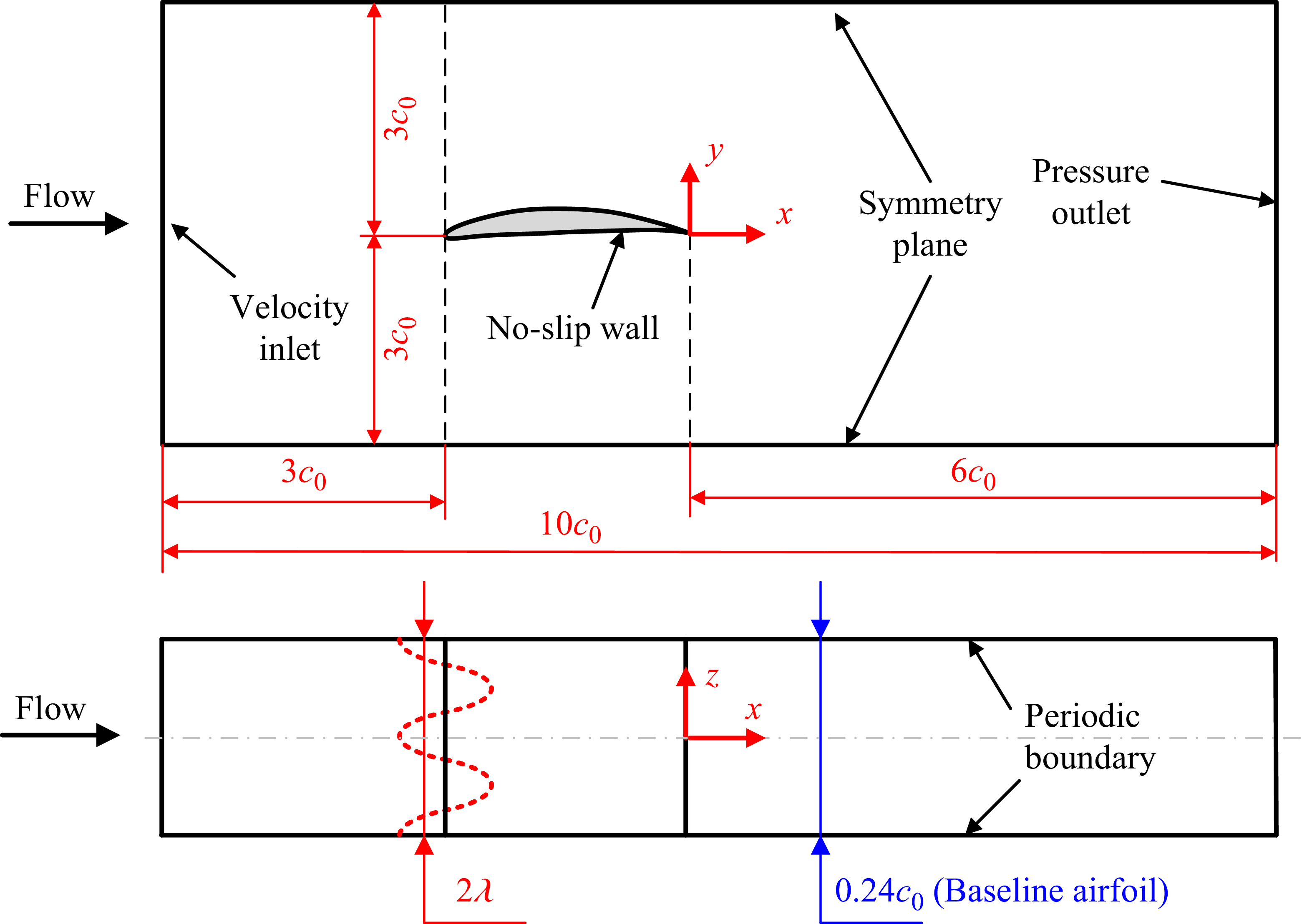

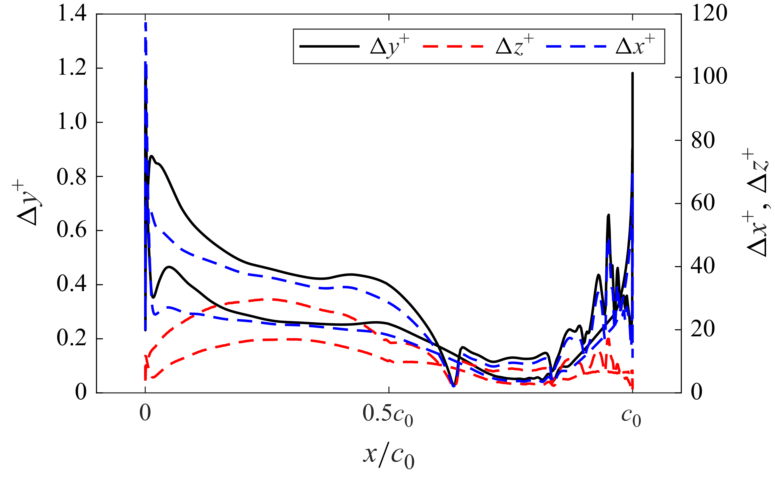


 ux¯

 k

 ux′
 p′

 Qn=5

 u¯x=0


 Cp

 ωxc0/u∞
 x/c0=−0.6
 x/c0=−0.5
 x/c0=−0.4
 x/c0=−0.3
 x/c0=−0.2
 x/c0=−0.1

 Qn=5


 Cp

 ωxc0/u∞
 x/c0=−0.6
 x/c0=−0.5
 x/c0=−0.4
 x/c0=−0.3
 x/c0=−0.2
 x/c0=−0.1


 Cl
 Cd
 ×

 ΔSPL


 Lp
 3⩽St⩽15
 3⩽St⩽15
 15⩽St⩽45
 15⩽St⩽45


 un,rms′
 ut,rms′

 δ∗
 θ
 H


 ut,rms′

 un,rms′

 un,rms′
 ut,rms′


 γij2(ω)
 x/c0=−0.05


 u∞=15∼35 m s−1
 u∞=40∼60 m s−1


