INTRODUCTION
Past extents of glaciers are reliable climatic proxies (e.g., Oerlemans, Reference Oerlemans2005; Blard et al., Reference Blard, Lavé, Pik, Wagnon and Bourlès2007) to reconstruct past climatic changes in continental areas (e.g., Martin et al., Reference Martin, Blard, Lavé, Condom, Prémaillon, Jomelli and Brunstein2018). Glacial extents are driven by the surface mass balance of glaciers, which is controlled by multiple climatic variables, including snowfall, temperature, albedo, relative humidity, insolation, and wind (e.g., Ohmura et al., Reference Ohmura, Kasser and Funk1992). Ideally, physical models can be developed to accurately link these climatic variables to glacial mass balances. This is the goal of surface-energy models that explicitly account for all atmospheric variables controlling glacial mass balance (e.g., Plummer and Phillips, Reference Plummer and Phillips2003; Rupper et al., Reference Rupper, Roe and Gillespie2009; Fitzpatrick et al., Reference Fitzpatrick, Radić and Menounos2017). However, some of the variables required by such models are often difficult to constrain, notably for past conditions. Other approaches, such as positive degree-day (PDD), models are simplified, easy-to-use alternatives (e.g., Braithwaite, Reference Braithwaite1995; Hock, Reference Hock2003; Gabbi et al., Reference Gabbi, Carenzo, Pellicciotti, Bauder and Funk2014). In certain climatic settings (e.g., low relative humidity, high solar insolation), however, PDD models may yield inaccurate estimates of surface mass balance, because they do not accurately capture processes such as sublimation or wind ablation (Sicart et al., Reference Sicart, Wagnon and Ribstein2005; Blard et al., Reference Blard, Wagnon, Lavé, Soruco, Sicart and Francou2011).
Several studies have shown that the response of alpine glaciers to climatic parameters is well captured by a glacier's equilibrium line altitude (ELA) (Meier, Reference Meier1962; Miller et al., Reference Miller, Bradley and Andrews1975; Porter, Reference Porter1975). ELA is the elevation at which annual accumulation is exactly balanced by annual ablation (e.g., Ohmura et al., Reference Ohmura, Kasser and Funk1992; Condom et al., Reference Condom, Coudrain, Sicart and Théry2007). This opens the door to even simpler empirical relationships linking ELAs and two climatic variables: summer temperatures and winter precipitation (e.g., Ohmura et al., Reference Ohmura, Kasser and Funk1992). Empirical studies have established regional relationships linking ELA to mean annual temperature (T) and precipitation (P) (e.g., Fox and Bloom, Reference Fox and Bloom1994; Condom et al., Reference Condom, Coudrain, Sicart and Théry2007). Indeed, the simple logarithmic calibration of Fox and Bloom (Reference Fox and Bloom1994), based on current glaciers in a restricted part of the tropical Andes (Peru, 5–17°S), accurately describes the spatial variability of present-day ELAs over the entire Andes Cordillera (10°N to 55°S; Condom et al., Reference Condom, Coudrain, Sicart and Théry2007).
Such a simple relationship between glacial mass balance and two climatic variables is useful, because it enables quick and accurate climatic projections (e.g., Condom et al., Reference Condom, Coudrain, Sicart and Théry2007) and paleoclimatic reconstructions (e.g., Martin et al., Reference Martin, Blard, Lavé, Condom, Prémaillon, Jomelli and Brunstein2018). However, such empirical relationships between ELA, P, and T are, in principle, only regionally valid, and regional variations of other confounding factors such as relative humidity, insolation, wind, and cloud cover may modify them. Thus, specific empirical relationships linking ELA, P, and T should ideally be determined for each climatic region using accurate present-day observations.
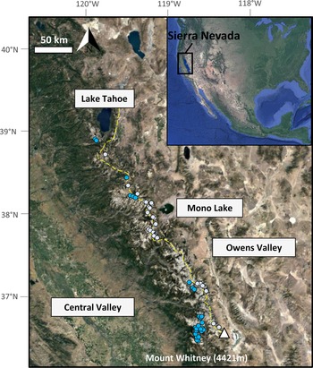
The Sierra Nevada is a midlatitude (36–41°N) North American mountain range situated between the Pacific Ocean and the arid deserts of Nevada, with summit elevations exceeding 4000 m above sea level (m asl) in the central part of the range (Fig. 1). At such high altitudes (i.e., 2900–4000 m asl), the westerly oceanic winds bring sufficient precipitation for promoting permanently glaciated areas between 36.4°N and 38.9°N (Pandey et al., Reference Pandey, Cayan and Georgakakos1999). This study aims to empirically calibrate the relationship between ELA, temperature, and precipitation for the Sierra Nevada, following the approach of Fox and Bloom (Reference Fox and Bloom1994) and Condom et al. (Reference Condom, Coudrain, Sicart and Théry2007). This empirical relationship can be used in future studies to reconstruct past climatic variables from the paleo-ELAs of glaciers from North America: that is, paleoprecipitation if paleotemperature is independently determined, or vice versa. This approach relies on the assumption that secondary climatic variables (other than precipitation and temperatures) are the same in the past as in the present.
Google Earth© images showing the regional setting of the Sierra Nevada range (western United States, inset) and the locations of the 57 glaciers studied (gray and blue dots). The yellow dashed line represents the crest of the Sierra Nevada. Glaciers east of the crest are gray dots; glaciers west of the crest are blue dots.

DATA AND METHODS
The main objective of this study was to determine an empirical relationship between local precipitation, 0°C isotherms, and present-day ELAs of Sierra Nevadan glaciers. This section describes the data and methods used to establish this relationship.
Data
PRISM temperature data
We chose to use the PRISM data set for climatological data, as it is a robust and widely used reanalyzed climatological product (PRISM Climate Group, Oregon State University, http://prism.oregonstate.edu, created July 2012) (Daly et al., Reference Daly, Halbleib, Smith, Gibson, Doggett, Taylor, Curtis and Pasteris2008, Reference Daly, Smith and Olson2015). We used the reanalyzed PRISM temperatures averaged over the 30 year normal period (1981–2010), gridded at a spatial resolution of 800 × 800 m. Glaciers behave as low-pass filters of the interannual climatic signal, averaging the climatic signal over the decadal timescale. This justifies the use of climatic data averaged over a period that precedes the date of the observed ELAs. Given their geometries and sizes, the 57 analyzed Sierra Nevadan glaciers integrate climate over a period that is representative of the previous 30 years (e.g., Zekollari and Huybrechts, Reference Zekollari and Huybrechts2015), meaning that the ELAs derived from the 2013 and 2012 images are likely representative of the 1981–2010 climatic period. The mean annual temperature corresponding to each glacier was assumed to be the value of the grid cell containing the glacier.
PRISM precipitation data
Mean annual precipitation was derived from PRISM data over the 30 year normal period (1981–2010) at a gridded spatial resolution of 800 × 800 m. This data set is spatially continuous, which is important for capturing the sharp spatial changes that are frequent in high-elevation terrains such as the Sierra Nevada. Moreover, the 30 year integration period of the data set smooths the interannual variability. The annual precipitation corresponding to each glacier was assumed to be the value of the cell in which the glacier is located.
Elevation data
For each precipitation and temperature value, we associated the elevation value of the PRISM data set of the corresponding cell. The digital elevation model (DEM) used for the PRISM normal data set is the National Elevation Dataset (Daly et al., Reference Daly, Halbleib, Smith, Gibson, Doggett, Taylor, Curtis and Pasteris2008). The average vertical uncertainty of the DEM expressed as the root mean-square error is 2.4 m (Gesch et al., Reference Gesch, Oimoen, Greenlee, Nelson, Steuck and Tyler2002); the horizontal resolution is 10 m, and 3 m in some local areas where really high resolution is available (Gesch et al., Reference Gesch, Oimoen, Greenlee, Nelson, Steuck and Tyler2002).
Landsat images of Sierra Nevadan glaciers (2012–2013)
To derive the ELAs of 57 Sierra Nevadan glaciers, we used clear-sky Landsat Thematic Mapper color images with a horizontal resolution of 15 m and the associated DEM available in Google Earth© (elevation uncertainty < 6 m; Sharma and Gupta, Reference Sharma and Gupta2014). Most glaciers were mapped and identified from images acquired between August and September 2013, although we also used images from August 2012, when 2013 images were not available in some areas. Summer 2013 was favored, as it corresponds to a relatively dry year, minimizing the risk of overestimating the glacial extent because of relict snow. When images from both years were available for the same glacier, comparison showed that the Sierra Nevadan ELAs of 2012 and 2013 were undistinguishable within uncertainties.
ELAs data set of 1972 for testing the ELA versus climate calibration
To test the robustness and the versatility of the calibration law derived from the 2012–2013 ELAs (see “Relationship between ELAs and Climate” for a description of this calibration; Eq. 3), we also considered another data set based on the oblique and vertical photographs of glaciers obtained during the aerial campaign of 1972 (August 23–24) in Sierra Nevada (Raub et al., Reference Raub, Brown and Post2006). These black-and-white pictures allowed determination of ELAs from 1972 with an uncertainty of 15 m (Raub et al., Reference Raub, Brown and Post2006). Raub et al.'s (2006) study identified 13 main basins in the Sierra Nevada, and we chose for each basin the glacier having the largest area in 1972. Two of them being debris-covered glaciers, our final 1972 test data set comprised 11 glaciers. Their areas range from 0.02 to 1.32 km2, with a mean of 0.38 km2 (Supplementary Table 2). Among these 11 glaciers, 4 have now disappeared (East Walker River Basin, Mokelumne River Basin, East Carson River Basin, Merced River Basin). The ELAs of these 11 glaciers were calculated using the same approach as the one applied for the glaciers’ data set based on the 2012–2013 images (see “Determination of ELAs”). For this test data set, we used PRISM Temperature and Precipitation reanalysis data from the 1941–1970 period (average of previous 30 year period), with a grid resolution of 4 × 4 km. PRISM temperatures of the 1941–1970 period were used to compute 0°C isotherms, applying the same method as the one applied to the 1981–2010 data set (see “Determination of 0°C Isotherm”).
Methods
Determination of ELAs
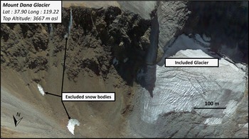
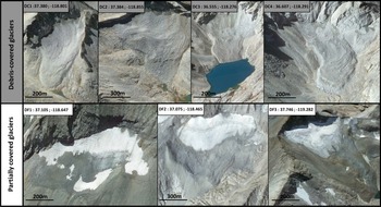
Perennial ice bodies were identified as glaciers if they fulfilled the following conditions (Figs. 2 and 3): (1) they were already described in a previous compilation of aerial photos from August 1972 (Raub et al., Reference Raub, Brown and Post2006); (2) they had an elevation range >30 m (Figs. 2 and 3); (3) they presented typical glacial features, such as crevasses (Fig. 2); and (4) their surfaces were only partially covered by debris. Because debris coverage may modulate ice melting (Clark et al., Reference Clark, Clark and Gillespie1994), we paid special attention to this criterion by analyzing the colors of the glaciers and clearly identify debris-covered areas. We discarded the fully covered glaciers from this calibration and included partially covered glaciers in the data set, with “partially covered” referring to glaciers whose surface is 10–90% debris free (Fig. 4).
September 2013 Landsat-Google Earth© image of four representative Sierra Nevadan glaciers. We used Google Earth digital elevation model (elevation uncertainty <6 m). Only the glacier on the right was included in the data set, as it is of sufficient size (elevation range >30 m), presents glacial features (crevasses), and is within a glacial cirque. The three excluded snow bodies on the left have elevation ranges <30 m.

Distribution of the elevation ranges of Sierra Nevadan glaciers in 2012 and 2013. Elevation range represents the difference between the headwall and toe elevations of each glacier. We used the digital elevation model displayed in Google Earth© (elevation uncertainty <6 m).

Examples of four debris-covered glaciers (top) and three partially covered glaciers (bottom) (Landsat-Google Earth© images). We consider a glacier as “partially covered” when 10–90% of its surface is free of debris. Only partially covered glaciers were included in the calibration.

We then calculated the ELA of each glacier using the toe-to-headwall altitude ratio (THAR) method, with a THAR coefficient of 0.5 (Charlesworth, Reference Charlesworth1957). While the THAR coefficient may range from 0.4 to 0.8 for glaciers worldwide (Benn and Lehmkuhl, Reference Benn and Lehmkuhl2000), a value of 0.5 was shown to be the most accurate for the Sierra Nevada (Moore and Moring, Reference Moore and Moring2013).
Determination of 0°C isotherm
To calculate the elevation of the 0°C isotherm at each glacier's location, we used the PRISM temperature and elevation data (Eq. 2). To compute this local 0°C isotherm, we used the temperature of the PRISM grid cell in which the glacier is located and combined this with the local mean annual environmental lapse rate (Lr). For this, we determined Lr for the Sierra Nevada range, using a linear regression between the 57 collected temperature and elevation cells (elevation also derived from the PRISM data set). We obtained a best-fit value of Lr = −5.20 ± 0.14°C/km (Fig. 5). This uncertainty corresponds to the 1σ confidence interval of the regression coefficient of the linear fit. To evaluate the accuracy of this Lr estimate, we also computed the Lr from 29 high-altitude (1128–2940 m asl) climatic stations of the Sierra Nevada from the National Weather Service Cooperative Observer Program (https://www.ncdc.noaa.gov, last accessed February 2021) (Supplementary Table 3). Using the same regression methodology, we found a best-fit value of Lr = −5.3 ± 0.5°C/km, which is similar within uncertainties to the Lr value derived from the PRISM data.
Mean annual temperature (T) vs. elevation (Z) for the 57 glaciers studied, derived from the PRISM data set (1981–2010). These data permit us to determine the average mean annual lapse rate (Lr) for the Sierra Nevada. Best-fit Lr is −5.20 ± 0.14°C/km (1σ).

Relationship between ELAs and climate
We followed the method of Fox and Bloom (Reference Fox and Bloom1994) and Condom et al. (Reference Condom, Coudrain, Sicart and Théry2007) to establish a simple relationship between the observed ELA (m asl), the elevation of the annual 0°C isotherm (Iso0, m asl), and mean annual precipitation (P, mm/yr). We first determined the modern ELA of Sierra Nevadan glaciers by analyses of Landsat satellite images available in Google Earth© from 2012 and 2013 using the THAR method (Charlesworth, Reference Charlesworth1957). Then, we subtracted the local 0°C isotherm (defined in “Determination of 0°C Isotherm”) from the ELA for each glacier to define the normalized snowline altitude (Y) as (Fox and Bloom, Reference Fox and Bloom1994):

where Iso0 is inferred from PRISM temperature data as:

where T is the local PRISM grid cell's mean annual temperature averaged over the 1981–2010 period (°C), Z is the mean elevation of the PRISM grid cell (m asl), and Lr is the average annual Lr of the studied region (°C/m) (Fig. 5).
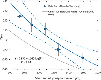
To smooth the data variability, we grouped and averaged the climatic and ELA data sets in five subclimatic regions based on mean annual precipitation. These subclimatic regions range from 800 to 1800 mm/yr, with a bin size of 200 mm/yr (Table 1). Using this data set, we established a relationship between Y and P:

where A and B are empirical variables specific to the region of interest. From their detailed survey of modern Peruvian and Bolivian glaciers in 21 subclimatic regions (5–17°S), Fox and Bloom (Reference Fox and Bloom1994) determined regional values of A (3427 m) and B (1148 m). Here, we used the same approach to calculate the values of A and B specific to Sierra Nevadan glaciers (Fig. 6).
Calibrated relationship between normalized snowline altitude (Y) and mean annual precipitation for the five subclimatic regions (see Table 1) of the Sierra Nevada (blue dots). The best-fit logarithmic calibration is shown by the blue curve (R 2 = 0.94; P value = 6.7 × 10⁻⁵; mean standard deviation of the mean (MSWD) = 0.62). The relationship was computed by taking into account the data uncertainties (Vermeesch, Reference Vermeesch2018). Dashed blue curves represent the 2σ confidence interval for external errors only. The gray curve is the calibration established for the tropical Andes by Fox and Bloom (Reference Fox and Bloom1994). The best-fit values of the empirical variables A and B in Eq. 6 for Sierra Nevada are 5150 ± 767 m and 1640 ± 244 m (1σ), respectively.

Averaged annual precipitation (mm/yr) and normalized snowline altitude (Y) (m) data used for the present Sierra Nevadan calibration for the five subclimatic regions, considering partially covered glaciers only (n = 57; see “Other Sources of Uncertainty”).a

a Mean annual precipitation and normalized snowline altitude are the arithmetic average values across all partially covered glaciers in each subclimatic region (based on mean annual precipitation bins of 200 mm/yr). Precipitation values are from the PRISM data set and cover the 1981–2010 climatic period, while normalized snowline altitudes are derived from 2012 and 2013 pictures. The 1σ values indicate the most realistic uncertainties associated with each subregion (see “Uncertainties on the Normalized Snowline Altitude and Mean Annual Precipitation” for uncertainty estimates).
b Computed as the standard deviation of each precipitation value of each subregion.
c Computed as the quadratic sum (Taylor series expansion) of the standard deviation/racine(n) of normalized snowline altitudes and of the analytical uncertainties in each subregion.
d The 1600–1800 subclimatic region is only composed of one glacier, inducing a null standard deviation for this subregion. The associated uncertainty is the error of the normalized equilibrium line altitude (ELA) computation itself.
Paleoclimatic reconstruction from ELAs derived from glacial landforms
For paleoclimatic reconstructions, once A and B are determined, it is possible to compute T from the paleo-ELA and P by combining Eqs. 1, 2, and 3:

Alternatively, if paleotemperature is constrained from an independent proxy, it is possible to compute P from Eq. 4:

Equations 4 and 5 may thus be used for paleoclimatic reconstructions.
In other situations, ELA positions may also be computed as a function of T and P. This could be useful to perform sensitivity tests, using independent proxies for paleotemperature and paleoprecipitation. Additionally, future projected P and T from global climate models may also be used as input in this equation to make first-order estimates of future ELA changes:

Results
Glacial inventory and ELAs
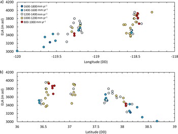
Our calibration data set consists of a total of 57 Sierra Nevadan glaciers, all located from 36.4°N to 38.9°N (Supplementary Table 1). Sierra Nevadan glaciers are most abundant around 37°N and are absent in two low-elevation zones between 37.4°N and 37.6°N and between 38.4°N and 38.8°N (Raub et al., Reference Raub, Brown and Post2006; Figs. 1 and 7). The 2012–2013 ELAs of these glaciers range from 2908 to 3957 m asl. They display a noticeable geographic variability, with two superimposed eastward and southward gradients (Fig. 7): along a west-east transect, ELAs rise from about 3000 m (120°W) to ~3800 m (118.5°W) (356 ± 31 m/decimal degree [DD] west-east gradient). Latitude has no visible impact on ELAs between 36.5°N and 37.5°N, but ELAs then drop from ~3800 m (37.5°N) to ~3000 m (38.5°N), corresponding to a south-north gradient of about −400 m/DD. This spatial variability results from increased precipitation to the west and decreased temperature to the north. Twenty-nine glaciers are located northeast of the crest in the rain shadow, whereas 28 of them are located southwest of the crest (Fig. 1). However, we did not observe any significant differences between these two sub–data sets, both yielding similar relationships between ELAs and climatic parameters. We thus considered the whole data set when establishing the calibration, without making any distinction between western and eastern glaciers.
Equilibrium line altitude (ELA) vs. (a) longitude and (b) latitude for the 57 glaciers analyzed (2012–2013). Colored dots represent glaciers of each subclimatic region: red for 800–1000, yellow for 1000–1200, blue-gray for 1200–1400, blue for 1400–1600, and dark blue for 1600–1800 mm/yr. From west to east, ELAs increase from ~3000 m asl (120°W) to ~3800 m asl (118.5°W), a west-east gradient of 356 ± 31 m/decimal degree (DD). Latitude has no visible impact on ELAs between 36.5°N and 37.0°N, but ELAs then decrease from ~3800 m asl (37.0°N) to ~3000 m asl (38.5°N), a south-north gradient of about −500 m/DD. This spatial variability results from increased precipitation toward the west and increased cooling toward the north. ELA uncertainties are provided in Supplementary Table 1.

Uncertainties on the normalized snowline altitude and mean annual precipitation
Each of the two variables involved in the calibration (Eq. 3)—mean annual precipitation and the normalized snowline altitude—has its own uncertainties that we estimated during each computation step.
To compute the 0°C isotherms (Eq. 2), we corrected the temperature of each glacier using the regional Lr (1σ uncertainty, 0.14°C/km; Fig. 5). The uncertainties on the normalized snowline altitude arising from this Lr correction range from 16 to 52 m. Additionally, we observe a scatter of the normalized snowline altitudes, Y, in each 200 mm/yr subclimatic region. This observed variability in each subregion represents another source of error. This uncertainty was computed for each subregion as the standard error of the mean, that is, σ(Y)/√n, σ(Y) being the standard deviation of the observed normalized snowline altitudes in each subclimatic region. Hence, the total uncertainty of the normalized snowline altitude of each subclimatic region combines the standard error of the mean and the uncertainty resulting from the Lr correction (Table 1). These errors were propagated using a Taylor series expansion.
The uncertainty associated with the PRISM precipitation data attributed to each subregion was computed as the standard deviation of all PRISM data points within each subregion. These uncertainties range from 35 to 61 mm/yr for the five subclimatic regions (Table 1).
Other sources of uncertainty
The resolution of the Landsat images used induces a vertical maximum uncertainty of 6 m on ELAs. Because the observed ELAs cover a range of more than 1000 m in this data set, this resolution does not represent an important source of uncertainty. We also tested the impact of the value of the THAR coefficient on our results. Using a THAR coefficient of 0.7 instead of 0.5 (global values range between 0.4 and 0.8; Benn and Lehmkuhl, Reference Benn and Lehmkuhl2000) shifts the computed ELA values by 0.7% on average and by 2.2% at most (Supplementary Table 1).
For each glacier, we attributed the temperature of the PRISM cell (800 × 800 m) in which the center of the glacier is located. This approximation may be a source of uncertainty, as a given glacier could belong to more than one grid cell. All the glaciers in our data set are smaller than a grid cell surface (0.64 km2). The largest glacier of the data set, Palisade Glacier, is 0.6 km2 (Supplementary Table 1). In an extreme case, however, a glacier could belong to up to four PRISM cells. Even if this case is unlikely, we estimated a maximum uncertainty by calculating the average absolute temperature difference of four adjacent cells of the PRISM grid data set (between 121–117°W and 40–36°N). This yields an average value of 0.25 ± 0.28°C. This spatially induced temperature uncertainty is on the order of 0.25°C, which remains reasonable. However, it may explain part of the data dispersion in the normalized snowline altitude versus precipitation space (Figs. 6 and 8).
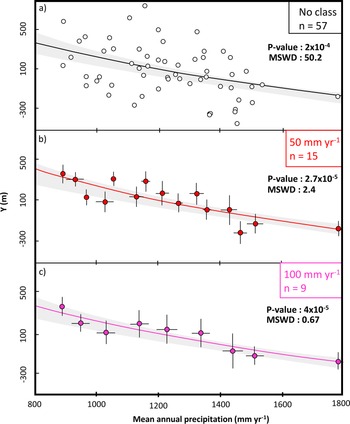
Relationships between normalized snowline altitude and mean annual precipitation computed from (a) the raw precipitation data set (no pre-averaging) and (b, c) precipitation data pre-averaged in subclimatic regions with bin sizes of (b) 50 and (c) 100 mm/yr. All three relationships are within the 2σ confidence interval of the relationship obtained with a subregional bin size of 200 mm/yr (shaded gray area; see Fig. 7). Each dot represents one subclimatic region. MSWD, mean standard deviation of the mean.

Uncertainties associated with the PRISM temperature and precipitation over the normal period (1981–2010) are difficult to evaluate. Daly et al. (Reference Daly, Halbleib, Smith, Gibson, Doggett, Taylor, Curtis and Pasteris2008) estimated uncertainties for the last PRISM climate-normal period (1971–2000) using cross-validation mean absolute error and a 70% prediction interval. Their results indicated that the highest uncertainties within the PRISM data set occur in the mountainous western United States, including the Sierra Nevada range, where uncertainties surrounding precipitation may reach 30% of the mean annual value and those for temperature may reach 1°C. We tested this PRISM-specific relative error of 30% for precipitation: it induced a drop of the mean standard deviation of the mean (MSWD) far below 1 (MSWD = 0.05). The MSWD, which is also known as the “reduced chi-square statistic,” is an indicator of the match between the model and the data, taking into account the agreement between the dispersion of the data and their attached uncertainties. This low MSWD value indicates that the data dispersion is much lower than expected from these uncertainties and that the 30% value reported by Daly et al. (Reference Daly, Halbleib, Smith, Gibson, Doggett, Taylor, Curtis and Pasteris2008) for precipitation probably overestimates the actual uncertainty. Hence, we consider that our error computation based on the standard deviation of precipitation in each subclimatic region (Table 1) is an accurate and sufficient predictor of the precipitation data dispersion.
Globally, the grid resolution of 800 × 800 m for the PRISM data could be a source of uncertainty if we consider that glaciers have a vertical extension and thus the top and the front of the glacier do not receive the same amount of precipitation and temperature. Although we did not try to explicitly quantify this uncertainty, this source of random error could also explain part of the data dispersion (Fig. 6).
Finally, although we did not identify a systematic correlation between the proportion of debris cover and the ELA position, we cannot exclude that the variability of the debris cover may explain part of the data scatter. Given that the elevation range covered by these small glaciers is on average ~100 m, the ELA scatter induced by the variable debris cover is limited and probably included in the noise of the data set (Supplementary Tables 1 and 2).
Normalized snowline versus P calibration
The normalized snowline values calculated for all glaciers using Eqs. 1 and 2 range between −457 and + 753 m, with a mean value of 162 ± 227 m. Mean annual precipitation for these glaciers ranges between 850 and 1791 mm/yr. After grouping the 57 glaciers into the five subclimatic regions of 200 mm/yr precipitation bins, we established the best fit between normalized snowline altitude and precipitation using the logarithmic model defined by Eq. 3 and a regression algorithm that accounts for data uncertainties (Vermeesch, Reference Vermeesch2018; Fig. 6). The best-fit values we obtained are A = 5150 ± 767 m and B = 1640 ± 244 m. Statistical parameters of this regression (R 2 = 0.94, P value = 6.7 × 10⁻³, MSWD = 0.62) indicate that it is accurate in describing the relationship between normalized snowline altitude and precipitation. An MSWD of 0.62, close to 1, shows that the magnitude of the uncertainties is realistic and is in agreement with the data dispersion.
DISCUSSION
Representativeness of the data set
We studied a representative glacier data set from the Sierra Nevada to obtain an accurate calibration. Our inclusion criteria avoid temporary snow bodies, thus yielding a total number of glaciers much lower than those in the previous compilation of Raub et al. (2006; 497 glaciers) and the Randolph Inventory Database 6.0 (GLIMS and NSIDC, 2005, updated 2018; 923 glaciers). However, these two inventories do not distinguish permanent glaciers from nonpermanent snowfields, and therefore may overestimate the actual number of glaciers. Fountain et al. (Reference Fountain, Glenn and Basagic2017) counted 157 glaciers in the Sierra Nevada based on a shear stress–threshold criterion to distinguish glaciers from perennial snowfields. However, they included debris-covered glaciers, whereas we only consider partially covered glaciers.
Moreover, the main reason that our data set is smaller than the Randolph Inventory Database is that we did not include glaciers with elevation ranges <30 m. The 57 partially covered glaciers used in our calibration have a mean elevation range of 107 m (standard deviation: 64 m). Their areas range from 3500 to 590,000 m2, for a mean value of 67,000 m2 (Supplementary Table 1). Glaciers having these typical sizes and geometries integrate climatic variables over the past 10 to 50 years (e.g., Oerlemans, Reference Oerlemans2012; Zekollari and Huybrechts, Reference Zekollari and Huybrechts2015). Hence, the selected calibration data set has the advantage of limiting the variability due to interannual fluctuations and justifies the use of the PRISM data set, which is averaged over the 30 years preceding the 2012–2013 glacier pictures.
Impact of the size of the subclimatic region on the calibration
The relationship between normalized snowline altitude and P (Eq. 3) is an easy-to-use tool to link precipitation and temperature to any glacial extent. However, secondary factors such as a glacier's orientation, atmospheric conditions, or local albedo can shift a particular glacier from the average relationship. Thus, we decided to minimize the noise generated by these secondary factors by averaging data from several glaciers based on the mean annual precipitation criteria. For our calibration, we used a 200 mm/yr interval to create subclimatic regions in which the P and normalized snowline altitude sub–data sets are averaged before performing the regression (see “Data”). As the width of this interval is an arbitrary choice, we tested the sensitivity of our model to the interval size by computing the calibration for intervals of 200 (Fig. 6), 100, and 50 mm/yr and for the raw data set (i.e., no binning interval; Fig. 8). The four relationships obtained are compatible within the 95% confidence interval, yielding similar parameters A and B (dashed blue lines in Fig. 6, light-gray shaded areas in Fig. 8). Notably, the calibration variables obtained for the raw data set (no binning) are A = 4905 and B = 1560, compatible within uncertainties with those derived from the 200 mm/yr binned data, A = 5150 ± 767 m and B = 1640 ± 244 m (Fig. 8). The computed P values are not significantly different between these different precipitation bin sizes, ranging from 2 × 10⁻⁴ for the whole data set to 2.7 × 10⁻⁵ for the 50 mm/yr bin (Fig.8). This test indicates that the data preclustering did not bias the obtained calibration, and we prefer to retain the parameters obtained with this 200 mm/yr interval. Moreover, the MSWD value decreases from 50.8 for the raw data to 0.62 for the 200 mm/yr bin (Fig. 8). An MSWD value of 0.62 indicates that this 200 mm/yr clustering accurately captures the variability arising from the data uncertainties, suggesting that our choice of bin size is representative of the real data dispersion (Fig. 8). Although different clustering bins may be used in further studies, our tests show that using a 200 mm/yr bin is justified and permits us to minimize the data scatter due to the secondary parameter control on the glacial mass balance.
Testing the calibration with a 1972 normalized snowline altitude data set of 11 representative glaciers
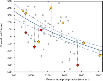
Figure 9 shows the agreement between the calibration curve and the test data set represented by 11 Sierra Nevadan normalized snowline altitudes observed in 1972. To test the robustness of our empirical normalized snowline altitude versus P relationship, we calculated the residuals between these 11 additional data and the calibration curve (Fig. 9). The obtained average residual value is 175 m. Using the present Sierra Nevadan Lr of 5.20 ± 0.14°C/km (see “Determination of 0°C Isotherm”), this corresponds to a paleotemperature uncertainty of 0.9°C. The size of this test data set (11 glaciers) is typical of a comprehensive paleoclimatic study that would reconstruct paleo-ELAs by dating moraines in a mountain range of a comparable area (e.g., Stansell et al., Reference Stansell, Polissar and Abbott2007; Roy and Lachniet, Reference Roy and Lachniet2010; Zech et al., Reference Zech, Terrizzano, Garcia Morabito, Veit and Zech2017). It is thus statistically representative and pertinent to provide a first-order estimate of the uncertainty attached to paleotemperature reconstruction from paleo-ELAs (~±1°C).
Comparison of the calibrated relationship with a test data set of 11 glacial equilibrium line altitudes (ELAs) observed in 1972. The 11 glaciers (red and yellow data points) used for this testing are based on PRISM climatic data of 1941–1970 and aerial photography of August 1972 (Raub et al., Reference Raub, Brown and Post2006). Yellow and red dots are respectively still existing (n = 7) and vanished glaciers (n = 4). Gray dots show the 2012–2013 glacial ELAs used to establish the calibration curve. Average residual between tested glaciers and the calibrated relationship (blue curve, dashed-blue curves represent 2σ confidence interval) is represented by the dark dashed-line distance and is on average 175 ± 197 m (standard deviation).

We also explored the cause of the disappearance of four glaciers within this data set (East Walker River basin, Mokelumne River basin, East Carson River basin, Merced River basin). Between the 1941–1970 and 1981–2010 periods, the PRISM data set indicates that temperature rose on average 1.1 ± 0.5°C at the locations of these four glaciers, while precipitation remained nearly constant or increased slightly (Supplementary Table 2). Combining temperature and precipitation measured over the 1981–2010 period at these four sites, our relationship (Fig. 6) yields theorical ELA1981–2010 values that are on average + 188 m higher than the summits of these four drainages. The disappearance of these four glaciers between 1972 and 2012 thus probably results from local warming that occurred over the last 40 years. This synchronous response of ELAs to warming confirms that these glaciers integrate the climatic parameters over 30 years or fewer.
Comparison of logarithmic and linear fits
Following several previous regional studies performed in the equatorial Andes (e.g., Fox and Bloom, Reference Fox and Bloom1994; Condom et al., Reference Condom, Coudrain, Sicart and Théry2007), we calibrated the normalized snowline altitude versus P relationship using a logarithmic fit. However, we also tested the statistical parameters of a linear fit, using the same data set: logarithmic fit, R 2 = 0.94, P value = 6.3 × 10⁻³; linear fit, R 2 = 0.94, P value = 6.7 × 10⁻³. The global calibration proposed by Greene et al. (Reference Greene, Seager and Broecker2002) is linear. In some particular cases, such as midlatitude glaciers fed by moderate to high precipitation (800–1800 mm/yr), a linear calibration seems to be a reliable approximation (Greene et al., Reference Greene, Seager and Broecker2002). However, their global linear calibration has only limited validity in extreme climatic conditions, notably in dry regions with precipitation of less than 200 mm/yr. For instance, their calibration is not able to reproduce the absence of glaciers in the central arid Andes (Ammann et al., Reference Ammann, Jenny, Kammer and Messerli2001). Linear glacier–climate calibrations should thus be considered with caution at regional scales, especially in arid areas. Although the Sierra Nevada is not subject to such a dry climate, our study aims to capture the regional specificity of the glacier–climate relationship. We therefore consider that the logarithmic calibration is probably a more accurate ELA–climate predictor (Fig. 6).
Comparison of the Sierra Nevadan and tropical Andean calibrations
Our ELA–climate calibration for Sierra Nevadan glaciers is statistically distinct from that established for the equatorial Andes by Fox and Bloom (Reference Fox and Bloom1994; Fig. 6). Our values for the empirical variables A and B (5150 ± 767 m and 1640 ± 244 m, respectively) are higher than their values for the Andes (A = 3427 m and B = 1148 m). In these two regions, the situations where ELAs and 0°C isotherms are equal are encountered at different annual precipitations (mean P = 1362 ± 94 mm/yr and 966 mm/yr for Sierra Nevada and tropical Andes, respectively). The differences between the two relationships should be considered with caution, as the discrepancy could lie in the nature of the climatological data set: our new calibration for the Sierra Nevada is based on reanalyzed temperature and precipitation, whereas the Andean calibration was established from discrete meteorological data from weather stations.
These potential intercontinental differences underscore the importance of local calibrations, when they exist, in computing paleoclimatic conditions from paleo-ELAs. However, despite these differences, the tropical Andean and Sierra Nevadan normalized snowline altitude values display quite comparable sensitivities to precipitation changes, the slopes of the relationships (the B parameters) being quite close for the two regions (Fig. 6). Our new calibration thus offers new and complementary constraints on the sensitivity to precipitation and temperature changes of alpine glaciers in an area of the American Cordillera that is wetter than the tropical Andes.
Implications for future paleoclimatic studies
Many paleoclimatic studies consider paleoglaciers to be paleothermometers, hypothesizing an equivalence between ELA and 0°C isotherm (Ramage et al., Reference Ramage, Smith, Rodbell and Seltzer2005; Vázquez-Selem and Lachniet, Reference Vázquez-Selem and Lachniet2017), while other studies limit their interpretation to ELA depression (Martini et al., Reference Martini, Kaplan, Strelin, Astini, Schaefer, Caffee and Schwartz2017). However, a glacier's extent is mainly controlled by two parameters: mean annual precipitation and temperature (Ohmura et al., Reference Ohmura, Kasser and Funk1992; Fox and Bloom, Reference Fox and Bloom1994; Condom et al., Reference Condom, Coudrain, Sicart and Théry2007). Hence, assuming that equilibrium lines and 0°C isotherms are strictly identical may induce inaccuracies in some situations. In particular, in regions fed by low precipitation (<200 mm/yr), the difference between the 0°C isotherm and ELA may reach 1000 m (Amman et al., Reference Ammann, Jenny, Kammer and Messerli2001; Carrasco et al., Reference Carrasco, Casassa and Quintana2005). Such a simplification could lead to bias larger than 5°C in temperature reconstruction. It is thus important to take into account both paleoprecipitation and paleotemperature in interpreting paleoglacial fluctuations.
Our empirical model is based on a relationship that only requires a paleo-ELA and a paleoprecipitation estimate to provide accurate reconstruction of paleotemperature. Compared with simpler approaches that directly consider paleo-ELAs as paleothermometers, this easy-to-use method has the potential to reduce the uncertainty of paleotemperature reconstruction from paleoglacial extents. Previous calibrations of the same model have either shown slight differences (Greene et al., Reference Greene, Seager and Broecker2002) or similarities (Condom et al., Reference Condom, Coudrain, Sicart and Théry2007) between midlatitude regions and the tropics, suggesting that paleoclimatic reconstruction from these models should use the closest empirical calibration. Although our relationship is established for the Sierra Nevada, its use for paleoclimatic reconstruction should for be encouraged for all midlatitude mountains ranges of North America, notably in American regions that are ice-free today (Owen et al., 2003; Marchetti et al., 2007).
CONCLUSION
Our calibration study established and tested a simple empirical model to link glacial ELAs of the U.S. Sierra Nevada with the main local climatic parameters (annual temperature and precipitation averaged over the previous 30 years). We demonstrated that the elevation difference between mean annual 0°C isotherm and ELA, the normalized snowline, is tightly linked with the mean annual precipitation (R 2 = 0.94, P value = 6.3 × 10⁻⁵). We provide here a simple tool to compute temperature from ELA and precipitation or precipitation from ELA and temperature. The uncertainty of temperature computed in this way is about 1°C at 1σ. This relationship will be especially useful for paleoclimatic studies, notably in regions where paleoglaciers are the unique paleoclimatic proxy.
Our study also compared the calibration relationships obtained from Sierra Nevadas and Andean glaciers (Condom et al., Reference Condom, Coudrain, Sicart and Théry2007). This comparison shows that different regions may require using specific calibration studies. When possible, using a local calibration has the potential to maximize the accuracy of glacial ELA-based paleoclimatic reconstructions. Further studies should be conducted in other mountain ranges to better document the interregional variability of this relationship between precipitation, temperature, and ELA.
Supplementary Material
The supplementary material for this article can be found at https://doi.org/10.1017/qua.2022.10
Acknowledgments
We thank Harry Zekollari for his very insightful comments on an earlier version of this article and Sylvie Cappelle for her expertise in handling several software programs used in this study. Robert Dennen carefully checked and edited the English. This work was funded by the ANR EroMed (PI: P-HB). The authors declare no competing interests.