





Impact Statement
Identifying the regions of a flow that most strongly influence its global behaviour is crucial in fluid mechanics, especially for unsteady or nonlinear flows where classical stability analyses can be difficult or expensive. In this work, we explore a data-driven approach based on vector quantisation and principal component analysis to cluster the flow domain into dynamically relevant regions. When applied to the canonical cylinder wake, the method naturally highlights regions associated with vortex shedding and structural sensitivity, showing that relevant flow patterns can be recovered directly from simulation data. The framework is then illustrated on the interaction of two synthetic jets, where the identified areas help interpret the mechanisms leading to symmetry breaking. Beyond these specific cases, the approach provides a simple and inexpensive way to analyse complex flows and identify regions where small perturbations may strongly influence the global dynamics.
1. Introduction
Understanding the intrinsic dynamics of complex fluid flows is crucial for diverse industrial fields, such as aerospace and wind engineering, the oil and gas industry or medicine. However, analysing these flows is challenging, as they involve a wide range of scales (in both space and time) (Peters Reference Peters2009), nonlinear interactions (Holmes et al. Reference Holmes, Lumley, Berkooz and Rowley2012) and experimental (Örlü Reference Örlü2017) and computationally (Jiménez Reference Jiménez2025) expensive simulations. An approach to address these drawbacks is modal decomposition techniques, which extract dominant flow structures and provide a reduced-order representation of the system (Taira et al. Reference Taira, Brunton, Dawson, Rowley, Colonius, McKeon, Schmidt, Gordeyev, Theofilis and Ukeiley2017). These methods have been proven to be very effective in capturing the essential physics of the flow while maintaining a moderate computational cost.
By identifying the dominant modes that govern the main dynamics of the flow, modal decomposition can be integrated with other strategies for specific applications such as instability analysis, flow control or optimisation. A complementary approach involves the identification of structural sensitivity zones, which highlight regions where small perturbations can have a significant global impact. As originally described by Giannetti & Luchini (Reference Giannetti and Luchini2007), structural sensitivity provides a powerful framework to detect regions of high receptivity to perturbations, which makes it particularly useful for guiding flow modifications.
A key challenge in computing structural sensitivity is its high computational cost, as traditional methods require solving both direct and adjoint problems (Giannetti & Luchini Reference Giannetti and Luchini2007). To address this limitation, clustering techniques provide an efficient, data-driven alternative to identify dynamically relevant flow regions directly from simulation data.
In this work, the term structural sensitivity zones is adopted to describe flow regions where small structural perturbations produce significant dynamic effects, and therefore small changes are most likely to influence the global dynamics. Here, such zones are identified through a data-driven approach based solely on direct flow simulations. This broadens the concept by allowing its application to unsteady and nonlinear regimes where adjoint solutions are difficult or expensive to compute.
Therefore, we explore the use of vector quantisation principal component analysis (VQPCA) to systematically identify structural sensitivity zones, reducing computational costs while maintaining accuracy. This clustering-based approach not only enables a deeper understanding of flow organisation but also offers valuable insights for applications such as reduced-order modelling and flow control. To the authors’ knowledge, this is the first application of VQPCA to a fluid dynamics problem for the identification of dynamically relevant regions and flow patterns.
From a conventional perspective, the computation of structural sensitivity maps typically involves combining direct and adjoint eigenfunctions. Luchini et al. (Reference Luchini, Giannetti and Pralits2008) developed a method based on this approach, which, despite its accuracy, can be computationally expensive, particularly for realistic three-dimensional flows. Recently, a novel approach (Corrochano & Le Clainche Reference Corrochano and Le Clainche2022) has been proposed to compute sensitivity maps at a reduced computational cost, since it requires only the computation of the direct problem. However, neither of these approaches can be extended to unsteady problems as they consider structural variations in the mean flow.
Even when sensitivity maps are available, identifying key regions for further analysis remains a challenge, particularly in complex flow environments. This issue is especially relevant when external modifications are introduced in these sensitive areas to influence global flow instabilities, as in the case of flow control. Techniques in this field are generally classified as active (e.g. oscillations and jets) or passive (e.g. cavities and vortex generators (Wang & Feng Reference Wang and Feng2018)). The process of identifying the most effective approach typically follows two main steps: first, selecting the appropriate technique and, second, optimising the control laws through numerical procedures. For nonlinear problems, genetic algorithms (Duriez et al. Reference Duriez, Brunton and Noack2017) are commonly used due to their ability to handle complex search spaces; however, they require hundreds of thousands of evaluations to achieve convergence. To make this computationally feasible, surrogated models are often used to approximate the response of the system, although the overall cost can still be significant (Pehlivanoglu & Yagiz Reference Pehlivanoglu and Yagiz2012). In this context, clustering techniques provide a powerful tool for analysing complex flow dynamics by identifying dynamically relevant regions. As a direct application, they can enhance the control optimisation step by reducing the search domain.
The primary objective of this work is to investigate a clustering technique as a tool to locate regions of maximum structural sensitivity in both steady and unsteady problems, substantially reducing computational cost. Clustering allows partitioning the flow field into dynamically relevant regions and provides a data-driven approach to identify areas where small perturbations can have a significant impact.
The proposed clustering method, VQPCA (Parente et al. Reference Parente, Sutherland, Dally, Tognotti and Smith2011), partitions the flow domain into distinct clusters. This study explores the potential connection between these clusters and structural sensitivity regions. The VQPCA method is based on principal component analysis (PCA), a well-established dimensionality reduction technique. Unlike traditional PCA, which operates on the entire dataset, VQPCA applies PCA locally within clusters, which are strategically chosen by the algorithm to optimise field reconstruction. While VQPCA has been widely used in combustion datasets to build reduced-order models (Amaduzzi et al. Reference Amaduzzi, D’Alessio, Pagani, Cuoci, Malpica Galassi and Parente2024; D’Alessio et al. Reference D’Alessio, Attili, Cuoci, Pitsch and Parente2021) and feature extraction (Zdybał et al. Reference Zdybał, D’Alessio, Attili, Coussement, Sutherland and Parente2023), recent work by Muñoz et al. (Reference Muñoz, Dave, D’Alessio, Bontempi, Parente and Le Clainche2023) has demonstrated its potential in non-reactive flows, where it effectively identifies and categorises regions based on their dynamics.
The approach is first applied to the flow past a cylinder, a case widely studied with well-established structural sensitivity regions. Given the extensive research on the inherent instabilities in this flow (Strykowski & Sreenivasan Reference Strykowski and Sreenivasan1990), it is the best candidate as a test case to calibrate the algorithm and validate our hypothesis. To further evaluate the robustness of the method, we analyse three datasets covering both two- and three-dimensional flows while varying the Reynolds number and spatial sampling.
After calibration, the algorithm is applied to the flow generated by two synthetic jets. These devices play a crucial role in various industrial applications, from improving fluid mixing (Wang & Menon Reference Wang and Menon2001) to optimising heat transfer (Pavlova & Amitay Reference Pavlova and Amitay2006) and even as alternative propulsion systems, inspired by the swimming motion of marine animals such as squids and jellyfish (Demont & Gosline Reference Demont and Gosline1988).
Subsequently, the identified structural sensitivity zones, determined through VQPCA, are analysed to explore their potential for modulating flow instabilities. Although these regions provide valuable information about the dynamics of the fluid, flow control naturally emerges as a potential application of this technique. To further illustrate this, two flow perturbation methods are examined: (i) active perturbation via point-force application and (ii) passive perturbation through the introduction of flow disruptors.
This study is organised as follows. Section 2 presents the methodology used, covering the clustering algorithm. The calibration and validation of this technique, performed on the flow around a circular cylinder, are detailed in § 3. Section 4 explores the application of the algorithm to synthetic jets, identifying structural sensitivity zones where a potential control strategy could be applied. Section 5 summarises the key conclusions.
2. Methodology
The governing equations describing an incompressible flow are the continuity and Navier–Stokes equations. They are written in a non-dimensional form as
 \begin{align} \nabla \cdot \boldsymbol u &= 0, \end{align}
 \begin{align} \frac {\partial \boldsymbol u}{\partial t} + \left ( \boldsymbol u \cdot \nabla \right ) \boldsymbol u &= -\nabla p + \frac {1}{\textit{Re}} \Delta \boldsymbol u, \end{align}
where
 $\boldsymbol u$
and
 $p$
are the non-dimensional velocity vector and pressure, respectively, and
 $Re = UL/\nu$
is the Reynolds number,
 $U$
and
 $L$
being the characteristic flow velocity and length and
 $\nu$
the kinematic viscosity of the fluid. These equations are non-dimensionalised with the units for length and time,
 $L$
and
 $L/U$
, respectively, as usual.
2.1. Structural sensitivity
In the field of fluid dynamics, Giannetti & Luchini (Reference Giannetti and Luchini2007) introduced the concepts of structural sensitivity and wavemakers. These concepts aim to identify flow regions where structural modifications in the stability problem lead to the most pronounced drift of the dominant linear stability eigenmode. A Reynolds decomposition is applied to the flow, which is expressed as a combination of the base flow or expectation (
 $\overline {\boldsymbol u}, \overline {p}$
) and an infinitesimal unsteady perturbation (
 $\boldsymbol u', p'$
), represented as
 \begin{equation*}\boldsymbol u = \overline {\boldsymbol u}+ \boldsymbol u' \ \ \text{and} \ \ p=\overline {p}+p'.\end{equation*}
Substituting this decomposition into (2.2), neglecting higher-order nonlinear terms in
 $\boldsymbol u'$
and introducing a forcing term, denoted as
 $\boldsymbol{f}$
, leads to
 \begin{equation} \frac {\partial \boldsymbol u'}{\partial t} + \left ( \overline {\boldsymbol u} \cdot \nabla \right ) \boldsymbol u' + \left ( \boldsymbol u' \cdot \nabla \right ) \overline {\boldsymbol u} = -\nabla p' + \frac {1}{\textit{Re}} \Delta \boldsymbol u' + \boldsymbol{f}. \end{equation}
For structural modifications, the forcing term is modelled to be proportional to the eigenmodal solution of the flow fluctuations. In linear flows, maximum sensitivity (maximum eigenvalue variation) is defined as the product of the magnitude of direct and adjoint velocity fields (Marquet et al. Reference Marquet, Sipp and Jacquin2008). Marquet et al. (Reference Marquet, Sipp and Jacquin2008) compared the impact of both base flow modifications and the application of a steady force. Following this approach, the present study examines both strategies within the identified sensitivity zones, considering the use of point forces and base flow modifications through the introduction of disruptors. In this context, ‘disruptors’ refer to square elements strategically placed within the domain, subject to specific wall conditions.
However, identification of structural sensitivity zones using conventional methods is highly computationally demanding, as it requires solving both the direct and adjoint Navier–Stokes equations. This challenge becomes even more prohibitive for unsteady applications (Rubino et al. Reference Rubino, Vitale, Colonna and Pini2020). To overcome this limitation, we propose an alternative approach based on VQPCA, which identifies potential structural sensitivity zones while only requiring the solution of the direct problem. This method not only extends the applicability of sensitivity analysis to unsteady flows, but also significantly reduces computational costs (Dave et al. Reference Dave, Swaminathan and Parente2022).
2.2. Clustering method: VQPCA
Vector quantisation via PCA is a local PCA technique introduced by Kambhatla & Leen (Reference Kambhatla and Leen1997) to mitigate reconstruction errors associated with the linearity of traditional PCA. By applying PCA locally, VQPCA constructs a more compact low-dimensional manifold that better captures the intrinsic structure of the data. This section provides an overview of the algorithm for this study. For more detailed information, the reader is referred to Parente et al. (Reference Parente, Sutherland, Dally, Tognotti and Smith2011).
In essence, VQPCA partitions the input dataset into distinct clusters of similar data points, acting as an unsupervised clustering algorithm. The input data consist of the flow dataset to be segmented, along with two crucial hyperparameters: the number of principal components retained in each cluster, denoted by
 $q$
, and the desired number of clusters,
 $k$
. The input dataset is structured as a matrix,
 $\mathbf{X} \in \mathbb{R}^{n \times p}$
, where
 $n$
represents the number of statistical observations to cluster and
 $p$
is the number of original variables.
Before applying machine learning algorithms to multivariate data, it is common practice to preprocess the dataset through centring and scaling. These operations are mathematically expressed as
 $\boldsymbol X'=(\boldsymbol X - \overline {\boldsymbol X})\boldsymbol D^{-1}$
, where
 $\overline {\boldsymbol X}$
and
 $\boldsymbol D$
represent the centring and scaling matrices, respectively. From this point on, the preprocessed matrix is referred to as
 $\boldsymbol X$
. The centring step subtracts the mean value of each variable, while scaling normalises each variable by the square root of its variance. For a more detailed explanation of these operations, the reader is referred to Parente & Sutherland (Reference Parente and Sutherland2013).
Figure 1 illustrates the steps undertaken by the algorithm. The process begins with the initialisation of the cluster centroids, which is selected to be a converged k-means solution (MacQueen Reference MacQueen1967) to accelerate convergence (D’Alessio et al. Reference D’Alessio, Parente, Stagni and Cuoci2020). For each cluster, the local eigenvector matrix,
 $\boldsymbol A^{(k)}$
, is computed, and a low-dimensional space, denoted as
 $\boldsymbol A_q^{(k)}$
, is defined by selecting the first
 $q$
principal components (
 $q \lt p$
). The reconstructed data,
 $\widetilde {\boldsymbol X}_q^{(k)}$
, are then obtained using the reduced basis. Principal component analysis is used here because the cluster assignment is based on local reconstruction error, for which PCA provides an optimal low-rank approximation in the least-squares sense. The reconstruction error at each grid point
 $i$
is calculated as
 $\epsilon _i^{(k)} = | \boldsymbol x_i - \widetilde {\boldsymbol x}_{i,q}^{(k)} |$
. Next, each data point is assigned to the cluster with the minimum reconstruction error, and the cluster centroids are updated. This process is repeated until the centroid variation falls below a predefined tolerance (Dave et al. Reference Dave, Swaminathan and Parente2022).
Scheme of the VQPCA algorithm, adapted from Dave et al. (Reference Dave, Swaminathan and Parente2022).

Figure 1 Long description
A flowchart illustrating the VQPCA algorithm process. The diagram starts with the input data matrix, which undergoes centering and scaling. This processed data matrix is then used for centroid initiation, leading to the partitioning of data into clusters. Local PCA is performed in each cluster, and data is reconstructed when assigned to a specific cluster from a q-dimensional manifold. Each point is assigned to the cluster that minimizes the reconstruction error. This iterative process continues until convergence is achieved, at which point the final cluster assignments are returned as the output.
The application of VQPCA to analyse complex fluid flows requires a specific arrangement of the data matrix, including compression along the temporal dimension. This enables the construction of a low-dimensional manifold that captures dominant flow patterns (Muñoz et al. Reference Muñoz, Dave, D’Alessio, Bontempi, Parente and Le Clainche2023) and partitions the domain into regions with similar dynamical behaviour. Although the primary aim of this clustering technique is to reveal the underlying flow organisation, one of its practical applications is flow control. Control strategies often rely on the introduction of perturbations (equation (2.3)) to modify the dynamics of the system, typically to suppress or enhance instabilities. Since VQPCA partitions the domain based on dominant flow dynamics, which are closely related to flow instabilities, it may highlight regions where perturbations have the greatest impact. This hypothesis is assessed and the method calibrated using the canonical case of a flow past a cylinder (§ 3).
The VQPCA method, proper orthogonal decomposition (POD)/PCA and dynamic mode decomposition (DMD) serve complementary purposes. The DMD technique represents spatio-temporal data through global modes, each associated with a specific temporal evolution, and can reveal localised flow-relevant regions (Spurin et al. Reference Spurin, Armstrong, McClure and Berg2023), although identifying the relevant modes requires an additional selection step. The POD/PCA approach provides orthogonal low-rank directions ranked by variance, but each mode may contain contributions from several frequencies. The VQPCA method embeds this idea locally: PCA bases are built within different clusters, and the domain is partitioned according to local reconstruction error. Thus, DMD identifies dynamically relevant global modes, whereas VQPCA identifies spatial regions with locally coherent temporal dynamics.
For noisy or experimental datasets, retaining only the dominant principal components within each cluster provides VQPCA with a limited implicit filtering effect, analogous to the low-rank singular value decomposition (SVD) truncation commonly used in DMD. Fluctuations not coherent with the dominant local temporal behaviour are expected to remain mainly in the reconstruction residual. Nevertheless, measured data still require standard preprocessing and robustness checks.
3. Application to the wake of a circular cylinder
3.1. Instabilities on the wake of a circular cylinder
The flow past a circular cylinder is a classic and well-understood benchmark problem in fluid dynamics. Despite its apparent simplicity, a range of flow regimes emerges as the Reynolds number increases. The Reynolds number is defined as
 $\textit{Re} = {U D}/{\nu }$
, where
 $U$
is the incoming free-stream velocity,
 $D$
is the cylinder diameter and
 $\nu$
is the kinematic viscosity of the fluid. At low Reynolds numbers (
 $\textit{Re} \lt 40$
), the flow remains steady and symmetric with respect to the mid-
 $Y$
and mid-
 $Z$
planes, and it is essentially two-dimensional. As
 $\textit{Re}$
increases to around
 $46$
, the first Hopf bifurcation occurs (Jackson Reference Jackson1987), resulting in an unsteady and periodic vortex shedding known as the von Kármán vortex street, although the flow remains two-dimensional. At approximately
 $\textit{Re} \approx 189$
, a secondary bifurcation triggers the onset of three-dimensionality, which depends on the spanwise length of the cylinder, defined as
 $L_z = 2\pi /\beta$
, where
 $\beta$
is the spanwise wavenumber (Barkley & Henderson Reference Barkley and Henderson1996).
The sensitivity of vortex shedding to small external perturbations (Kovasznay Reference Kovasznay1949) and geometrical modifications (Stansby Reference Stansby1974) at low Reynolds numbers has been well established in previous studies. Strykowski & Sreenivasan (Reference Strykowski and Sreenivasan1990) identified specific regions in the wake where local alterations exert the greatest influence on the global flow. Their analysis, involving structural perturbations introduced through smaller cylinders, aimed to control the onset of flow instability and was supported by both experimental and computational investigations. Later, Giannetti & Luchini (Reference Giannetti and Luchini2007) introduced a structural sensitivity analysis based on linearisation around the base flow, defining these critical areas as structural sensitivity zones. In particular, the regions identified in the two studies do not overlap completely. This discrepancy arises because the former captures the effect of perturbations on both the base flow and its fluctuations, while the latter considers only linear perturbations around a steady base flow.
In this section, we apply VQPCA to the cylinder datasets presented in § 3.2 to determine whether the same structural sensitivity zones can be recovered. These results serve to validate the proposed clustering-based approach and to calibrate the hyperparameter selection for future applications.
3.2. Datasets
This study employs three distinct datasets representing the wake behind a circular cylinder at different Reynolds numbers. Two datasets correspond to two-dimensional simulations at Reynolds numbers of
 $60$
and
 $100$
, while the third represents a three-dimensional flow at a Reynolds number of
 $280$
, with a spanwise domain length of
 $6.99D$
. For clarity, these cases are referred to as 2D60, 2D100 and 3D280 throughout the text.
Numerical simulations were conducted using the open-source spectral element solver (Fischer et al. Reference Fischer, Lottes and Kerkemeier2008), which solves the incompressible continuity and Navier–Stokes equations in non-dimensional form ((2.1) and (2.2)). The computational domain extends from
 $x \in [-15, 50]D$
in the streamwise direction and
 $y \in [-15, 15]D$
in the normal direction. Boundary conditions were implemented following the set-up described by Barkley & Henderson (Reference Barkley and Henderson1996). At the inlet and on the upper and lower boundaries, Dirichlet conditions were applied for the velocity field (
 $u_x = U = 1$
,
 $u_y = 0$
and
 $u_z = 0$
in the three-dimensional case), while Neumann conditions were used for pressure. Standard outflow conditions were imposed at the outlet, consisting of Neumann conditions for velocity and Dirichlet conditions for pressure. No-slip conditions were enforced on the cylinder surface. The two-dimensional domain consists of
 $600$
rectangular macro-elements, each discretised with
 $p+1$
Gauss–Lobatto–Legendre points, where
 $p = 9$
is the polynomial order. For the three-dimensional simulation, the spanwise direction is extruded using
 $64$
equispaced planes over a domain length of
 $L_z=6.99D$
, with periodic boundary conditions imposed at the spanwise ends. This length corresponds approximately to one complete wavelength of a three-dimensional perturbation with non-dimensional spanwise wavenumber
 $\beta =0.9$
, since
 $\lambda _z=2\pi /\beta \simeq 6.98D$
. According to the Floquet stability analysis of Barkley & Henderson (Reference Barkley and Henderson1996), this wavenumber belongs to the long-wavelength instability branch associated with mode A at
 $\textit{Re}=280$
. Additional details of the simulation set-up and parameters can be found in Vega & Le Clainche (Reference Vega and Le Clainche2020) and Le Clainche et al. (Reference Le Clainche, Pérez and Vega2018).
Although the three datasets share the same computational domain in the
 $x$
–
 $y$
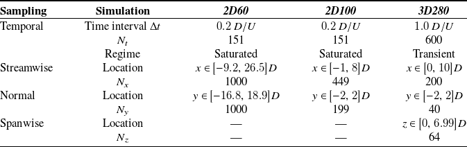
plane, they differ in their temporal and spatial sampling. Details of these sampling schemes are provided in table 1. The temporal sampling is characterised by the number of equispaced snapshots,
 $N_t$
, collected during the transient or saturated regime, after the simulations have converged in time. The corresponding time intervals,
 $\Delta t$
, are also presented for each of the three test cases. The temporal sampling of the three-dimensional simulation is limited to transient data due to an instability in the spanwise direction, which evolves over time as the flow saturates in the other spatial directions (Le Clainche et al. Reference Le Clainche, Pérez and Vega2018).
Summary of the temporal and spatial sampling of each dataset. Temporal sampling includes the number of snapshots collected (
 $N_t$
), their time interval (
 $\Delta t$
) and the flow regime (saturated or transient). Spatial sampling includes the number of grid points (
 $N_x$
,
 $N_y$
,
 $N_z$
) and their locations in the streamwise, normal and spanwise directions.

Table 1 Long description
The table presents a comparison of temporal and spatial sampling for three datasets: 2D60, 2D100, and 3D280. It has four rows and five columns. The columns are labeled Sampling, Simulation, 2D60, 2D100, and 3D280. The rows are labeled Temporal, Streamwise, Normal, and Spanwise. Under Temporal, the sub-rows are Time interval, Nt, and Regime. Under Streamwise, Normal, and Spanwise, the sub-rows are Location and Nx, Ny, and Nz respectively. For 2D60, the Time interval is 0.2 D/U, Nt is 151, and Regime is Saturated. The Streamwise Location is x ∈ [-9.2, 26.5]D, and Nx is 1000. The Normal Location is y ∈ [-16.8, 18.9]D, and Ny is 1000. For 2D100, the Time interval is 0.2 D/U, Nt is 151, and Regime is Saturated. The Streamwise Location is x ∈ [-1, 8]D, and Nx is 449. The Normal Location is y ∈ [-2, 2]D, and Ny is 199. For 3D280, the Time interval is 1.0 D/U, Nt is 600, and Regime is Transient. The Streamwise Location is x ∈ [0, 10]D, and Nx is 200. The Normal Location is y ∈ [-2, 2]D, and Ny is 40. The Spanwise Location is z ∈ [0, 6.99]D, and Nz is 64.
Contour plots of the velocity components of (a,b) 2D60 and (c,d) 2D100 in their sampling domain.

Figure 2 Long description
The image contains four contour plots. Panel A shows the streamwise component, ux, of 2D60. The x-axis is labeled x/D and ranges from -9 to 25. The y-axis is labeled y/D and ranges from -15 to 15. The color scale ranges from -1 to 1. Panel B shows the normal component, uy, of 2D60. The x-axis is labeled x/D and ranges from -9 to 25. The y-axis is labeled y/D and ranges from -15 to 15. The color scale ranges from -0.6 to 0.6. Panel C shows the streamwise component, ux, of 2D100. The x-axis is labeled x/D and ranges from -1 to 8. The y-axis is labeled y/D and ranges from -2 to 2. The color scale ranges from -1 to 1. Panel D shows the normal component, uy, of 2D100. The x-axis is labeled x/D and ranges from -1 to 8. The y-axis is labeled y/D and ranges from -2 to 2. The color scale ranges from -0.5 to 0.5.
For spatial sampling, the number of grid points (
 $N_x$
,
 $N_y$
,
 $N_z$
) in the streamwise, normal and spanwise directions is specified, along with their respective locations (
 $x$
,
 $y$
,
 $z$
). The centre of the cylinder is located at the origin of the coordinate system (
 $x = 0$
,
 $y = 0$
), and in the three-dimensional case, its length is given by
 $L_z$
.
Figure 2 shows contour plots of the streamwise velocity component,
 $u_x$
, and the normal velocity component,
 $u_y$
, for the 2D60 and 2D100 datasets. As expected, the first instability is evident in both cases, marked by the vortex shedding downstream of the cylinder, consistent with Reynolds numbers exceeding
 $46$
. Additionally, these plots highlight the differences in spatial sampling, displaying the complete computational domain used for the data analysis, as detailed in table 1.
Figure 3 displays the streamwise velocity component in the middle
 $x$
–
 $y$
plane and the three-dimensional spanwise vorticity, defined as
 $\omega _z = {\partial u_y}/{\partial x} - {\partial u_x}/{\partial y}$
, for the 3D280 case. As shown, this case exhibits structures not only in the
 $x$
–
 $y$
plane but also along the spanwise direction, indicating that the second bifurcation has occurred. This is consistent with the Reynolds number exceeding
 $189$
and the spanwise length of the cylinder being sufficient for the instability to develop.
(a) Streamwise component of the velocity
 $u_x$
and (b) vorticity
 $\omega _z$
of 3D280.

The variety of datasets allows for a comprehensive evaluation of the algorithm’s performance under (i) varying operating conditions and (ii) different spatial dimensionalities. This is achieved by analysing two- and three-dimensional datasets that capture diverse spatial domains at different Reynolds numbers.
3.3. Data preparation
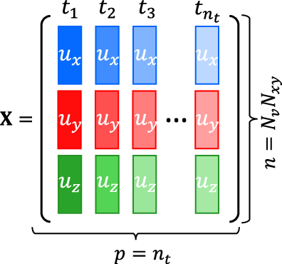
The datasets have been structured to ensure consistency in the application of the clustering technique. Each dataset is organised into a matrix
 $\boldsymbol X\in \mathbb{R}^{n\times p}$
, where
 $n$
represents the number of statistical observations to be clustered and
 $p$
is the number of variables describing each observation. For convenience, the total number of grid points in space is defined as
 $N_{xyz} = N_x N_y N_z$
, with
 $N_z = 1$
for the two-dimensional cases. The number of selected fluid variables (e.g. velocity components and pressure) is denoted by
 $N_v$
, taking values
 $2$
and
 $3$
for two- and three-dimensional cases, respectively (representing
 $u_x$
,
 $u_y$
and
 $u_z$
), and the total number of snapshots included in the analysis is
 $n_t$
. Therefore, each spatial-variable location is treated as an observation described by its temporal evolution over the selected snapshots. Although centring and scaling normalise the selected variables and the PCA step reduces redundancy among them, the clustering may still depend on the physical fields used to construct the input matrix. Other variables, such as pressure, vorticity or the
 $Q$
-criterion, could be included to emphasise specific flow features; here, velocity components are retained because they are the variables most commonly considered in the structural sensitivity literature.
Following Muñoz et al. (Reference Muñoz, Dave, D’Alessio, Bontempi, Parente and Le Clainche2023), the data are organised in matrices with dimensions
 $n=N_{xyz} N_v$
and
 $p=n_t$
. Figure 4 schematises the construction of the matrices.
3.4. Clustering results
This section presents the results of the VQPCA implementation in the cylinder datasets (§ 3.2), described in § 3.3, with the goal of identifying structural sensitivity zones.
Summary of the number of snapshots selected (
 $n_t$
) and corresponding wave cycles in each case.

Table 2 Long description
The table compares the number of snapshots selected and the corresponding wave cycles for three simulations: 2D60, 2D100, and 3D280. It has four columns labeled Simulation, 2D60, 2D100, and 3D280, and two data rows. The first row, Snapshots selected n_t, gives values of 30 for 2D60, 30 for 2D100, and 40 for 3D280. The second row, Wave cycles on the interval, gives values of 1 for 2D60, 1 for 2D100, and 10 for 3D280.
Scheme of the matrix
 $\boldsymbol X$
.

To begin the analysis, the first step involves calibrating the hyperparameters of the algorithm. To capture the most energetic direction in time, the number of principal components retained is fixed at
 $q=1$
. The number of selected snapshots,
 $n_t$
, is chosen to cover a full number of oscillation cycles in periodic flows, while being kept as low as possible to reduce computational cost. The number of clusters,
 $k$
, is determined by minimising the Davies–Bouldin index (DBI) (Davies & Bouldin Reference Davies and Bouldin1979), which quantifies cluster quality by balancing intra-cluster similarity and inter-cluster separation. Section 3.4.1 details the hyperparameter calibration using the 2D100 dataset as a reference case. This dataset was selected due to its lower spatial dimensionality, which enables faster evaluations during the calibration phase. Once the optimal parameters are identified, the algorithm is systematically applied to the remaining datasets. The results are then analysed and compared to validate the methodology, as discussed in § 3.4.2.
The computational cost of VQPCA is mainly controlled by the number of spatial-variable observations,
 $N_{xyz}N_v$
, the number of selected snapshots,
 $n_t$
, the number of clusters,
 $k$
, the number of retained principal components,
 $q$
, and the number of iterations required for convergence. Since in the present applications
 $n_t$
,
 $k$
and
 $q$
are small, the cost scales approximately linearly with the number of sampled grid points, which makes the method suitable as a post-processing tool within computational fluid dynamics workflows. For reference, the algorithm took 42 s to converge for the 2D100 dataset (
 $N_{xy}=89351$
) using
 $k=3$
,
 $q=1$
and
 $n_t=30$
, on a single core of an Intel Xeon E5-2603 processor.
3.4.1. Hyperparameter calibration
The first hyperparameter to be defined is the number of selected snapshots, denoted as
 $n_t$
. Following the aforementioned guidelines,
 $n_t$
is set to
 $30$
for both 2D60 and 2D100, capturing one full vortex-shedding cycle during the quasi-steady regime. This is sufficient due to the two-dimensional nature of the flow and the regularity of the shedding pattern, which is well represented within a single period. For 3D280, however, a larger value of
 $n_t=40$
is chosen to represent 10 cycles, starting from the 100th cycle, after the two-dimensional shedding has reached a quasi-saturated state, but while the spanwise instability is still evolving. In the three-dimensional case, extended sampling ensures that the more complex and potentially asymmetric three-dimensional structures are adequately captured. This information is summarised in table 2.
The second and final hyperparameter to be selected is the number of clusters
 $k$
. To investigate its effect, figures 5 and 6 show the clustering indices obtained for the streamwise and normal velocity components (
 $u_x$
and
 $u_y$
, respectively), in a range of
 $k \in [2,8]$
. As
 $k$
increases, the clustering algorithm refines the domain segmentation by either splitting existing regions or introducing entirely new ones. This behaviour reflects the ability of the algorithm to identify increasingly localised dynamics within the flow. In particular, while smaller values of
 $k$
capture the global structure of the flow, larger values provide a more granular view that may better align with local instabilities or flow features relevant to control.
Clustering contours corresponding to the streamwise velocity component,
 $u_x$
, of the reference case 2D100. Each subfigure corresponds to a number of clusters,
 $k \in [2,8]$
.

Same as figure 5 for the normal component of the velocity,
 $u_y$
.

Figure 6 Long description
Panel k=2: A heat map showing the clustering contours for the normal velocity component of the 2D100 cylinder wake with two clusters. The x-axis is labeled x/D and ranges from -1 to 8. The y-axis is labeled y/D and ranges from -2 to 2. The colors identify the two different cluster labels. Panel k=3: A heat map with the same axes showing the clustering solution with three clusters, represented by three different cluster labels. Panels k=4, k=5, k=6, k=7, and k=8 show the corresponding clustering solutions with four, five, six, seven, and eight clusters, respectively. In all panels, the colors represent categorical cluster labels and do not indicate velocity magnitude. As the number of clusters increases, the flow domain is partitioned into a progressively larger number of regions.
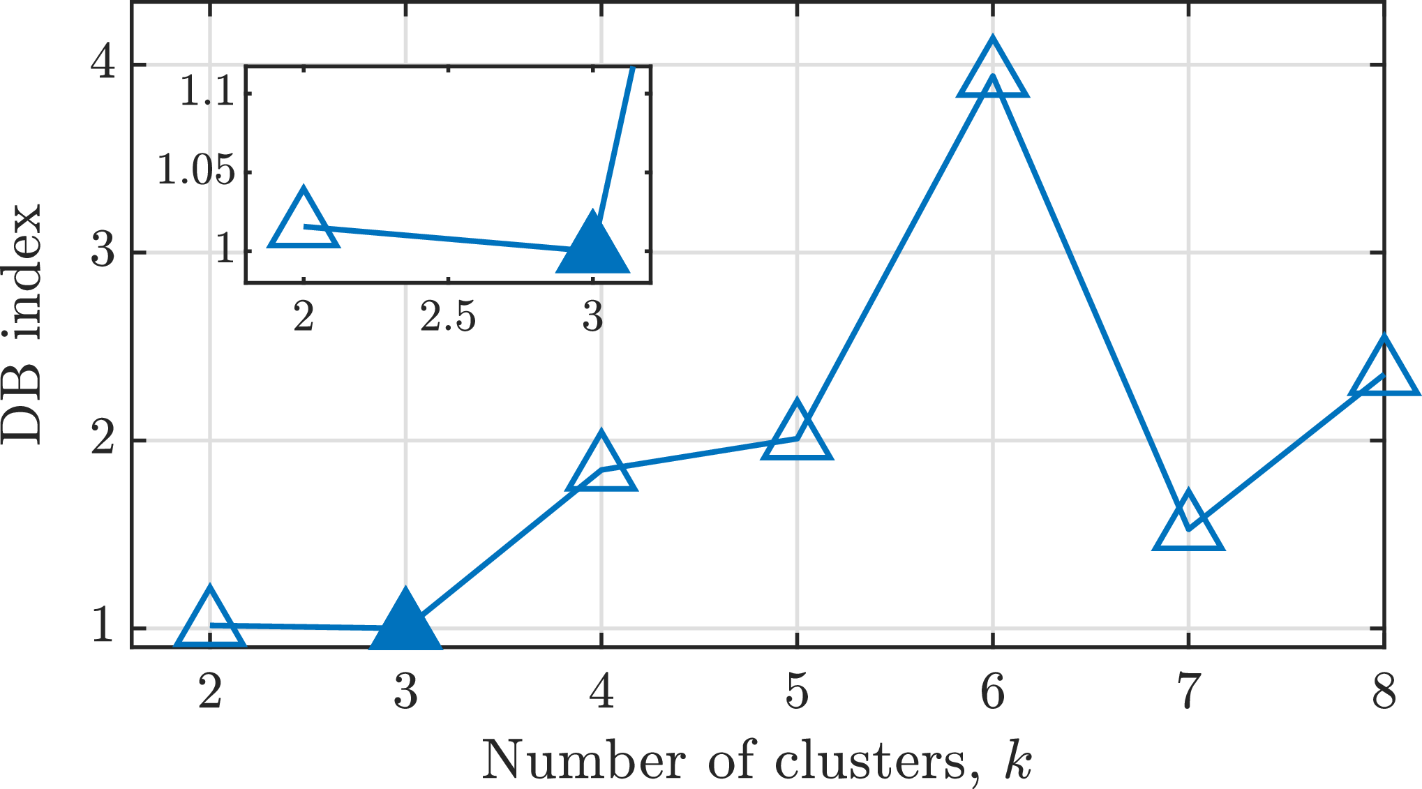
As the number of clusters increases, smaller scales are captured. However, the objective is not simply to solve smaller structures, but to identify a partitioning in which each cluster exhibits strong internal coherence in its reduced-dimensional representation while remaining as distinct as possible from the others. In this context, an ideal clustering solution maximises intra-cluster similarity and inter-cluster dissimilarity, leading to high orthogonality between clusters. To determine the optimal number of clusters, we employ the DBI, a commonly used metric based on Euclidean distances that quantifies this trade-off. A lower DBI indicates better clustering performance. Figure 7 shows the DBI values obtained for the 2D100 dataset as the number of clusters varies from
 $k=2$
to
 $k=8$
. According to this criterion, the optimal clustering corresponds to
 $k=3$
, which is marked in the figure with a filled symbol.
The DBI for the clustering results of 2D100 with
 $k\in [2,8]$
. Optimal solution is represented with a filled symbol.

The clustering contours for the streamwise velocity component
 $u_x$
, shown in figure 5 for the optimal configuration (
 $k=3$
), reveal two lobe-shaped regions, while the third cluster spans the remainder of the domain. These lobe structures closely resemble those reported in structural sensitivity analyses of the circular cylinder wake, such as figure 20 in Strykowski & Sreenivasan (Reference Strykowski and Sreenivasan1990) and figure 17 in Giannetti & Luchini (Reference Giannetti and Luchini2007), although obtained using different methodologies and Reynolds numbers. As discussed in § 1, structural sensitivity zones highlight flow regions that are particularly receptive to perturbations. Introducing minor alterations within these zones can influence the onset of instabilities, either delaying or promoting them, which facilitates the application of flow control strategies.
As the number of clusters or retained principal components increases, the characteristic lobe shapes become less visible, with the domain being divided into more granular regions, including those away from the central wake. Moreover, the structure of this optimal clustering solution shows a strong resemblance to the spatial distribution of the first DMD mode, specifically the norm of its magnitude, defined as
 $N_1 = \sqrt { {|u_x^1|}^2 + {|u_y^1|}^2 }$
(figure 8
a). This DMD mode is known to represent the global wake motion and is closely related to the fundamental flow instability, further reinforcing the relevance of the clustering results.
(a) Norm
 $N_1$
and (b)
 $\mathcal{R}(u_y^1)$
of the first DMD mode at frequency
 $f_1$
. (c) Power spectral density of the first principal component for each cluster
 $k$
,
 $\text{PSD}(\text{PC}_1^{(k)})$
, of the optimal clustering solution.

Figure 8 Long description
Panel A: A contour plot displays the norm of the absolute value of the first DMD mode. The x-axis is labeled x/D and ranges from 0 to 8. The y-axis is labeled y/D and ranges from -2 to 2. The color scale on the right indicates values from -1 to 1. Panel B: Another contour plot shows the real part of the normal velocity component of the first DMD mode. The axes and color scale are the same as in Panel A. Panel C: A line graph presents the power spectral density for each cluster. The x-axis is labeled f [Hz] and ranges from 0 to 11. The y-axis is labeled PSD [dB] and ranges from -100 to 0. Three lines represent different clusters, with k=1 in blue, k=2 in orange, and k=3 in green. The graph shows variations in power spectral density across different frequencies for each cluster.
Figure 6, which illustrates the clustering solution for
 $u_y$
, supports the observation that the cluster structures change significantly as the number of clusters increases. This analysis focuses on the optimal case with
 $k=3$
, where the domain is divided into wake regions that closely resemble the configuration shown in figure 2(d). The similarity becomes even more evident when the clustering is compared with the real part of the first DMD mode of
 $u_y$
(figure 8
b), which is associated with the oscillation frequency of the wake. In particular, the clustering solution is symmetric, reflecting the inability of the algorithm to distinguish between regions above and below the cylinder along the normal direction (
 $y$
).
To further confirm this correspondence, we compute the power spectral density of the principal component for each cluster
 $k$
, denoted
 $\text{PSD} \left (\text{PC}_1^{(k)}\right )$
. The results are shown in figure 8(c). The frequency of the first DMD mode, denoted as
 $f_1$
, corresponds to the wake oscillation frequency. The spectral density of clusters
 $1$
and
 $3$
peaks at
 $f_1$
, indicating a strong correlation with this mode. In contrast, the principal component of cluster
 $2$
shows a maximum spectral density at
 $f=0$
, revealing a steady region.
These results demonstrate that the DBI provides an optimal solution closely related to the flow physics. It effectively identifies (i) regions that correspond to the structural sensitivity of the first instability in the wake, particularly with respect to the streamwise velocity component, and (ii) the first DMD mode, which is associated with the wake behind the cylinder generated by this instability. For consistency in the analysis and subsequent comparisons,
 $k=3$
is fixed from this point onward.
3.4.2. Robustness assessment of the method and its calibration
Having selected all parameters based on a reference case, the next step is to assess the robustness and reliability of both the method and its calibration. To this end, clustering results are compared in the three cylinder datasets (2D60, 2D100 and 3D280), and the main assumptions underlying the method are evaluated. Specifically, the clustering procedure is shown to extract physically meaningful features from the flow. In particular, clustering based on the streamwise velocity component,
 $u_x$
, was found to reveal regions potentially associated with structural sensitivity zones.
The comparison described above is illustrated in figure 9, which shows the clustering results for the streamwise and normal velocity components across the three cases. The same hyperparameter values used in the previous analysis are maintained, namely
 $k=3$
and
 $n_t$
as listed in table 2. For the three-dimensional case, results are shown on the mid-plane in the
 $x$
–
 $y$
direction. In all cases, the characteristic lobes previously identified in 2D100 are present and their structure aligns well with the existing literature (Giannetti & Luchini Reference Giannetti and Luchini2007; Strykowski & Sreenivasan Reference Strykowski and Sreenivasan1990). Moreover, as the Reynolds number increases, the lobes become smaller and shift closer to the cylinder, which is consistent with experimental observations (see figure 20 in Strykowski & Sreenivasan (Reference Strykowski and Sreenivasan1990)).
This agreement is expected primarily when the flow dynamics is dominated by a small number of coherent instabilities. In such regimes, global decompositions, such as DMD and POD/SVD, can recover comparable dominant dynamics (Gómez et al. Reference Gómez, Le Clainche, Paredes, Hermanns and Theofilis2012), while VQPCA performs low-rank PCA reconstruction locally within each cluster. Therefore, VQPCA can identify the spatial subregions in which this dominant dynamics is most strongly expressed, providing a physical explanation for the observed similarity between some clusters and established structural sensitivity regions. Nevertheless, these clusters should be interpreted as data-driven indicators of dynamically relevant or structurally sensitive regions, rather than as exact replacements for adjoint-based sensitivity maps. The present results support this interpretation for nonlinear laminar flows dominated by coherent structures. Its extension to transitional regimes appears plausible, but its applicability to broadband, strongly multiscale or fully turbulent flows remains to be assessed.
Clustering solution for the three cylinder datasets (cases 2D60, 2D100 and 3D280). Top row: streamwise velocity component,
 $u_x$
. Bottom row: normal velocity component,
 $u_y$
.

The lower spatial resolution of the 3D280 dataset results in less defined cluster contours in figure 9. However, the algorithm yields consistent results across all cases, despite variations in Reynolds number, mesh characteristics (including domain extent, discretisation and spatial dimensionality) and the inclusion of the third velocity component. Additional analysis of the three-dimensional case is provided in Appendix A of the supplementary material available at http://doi.org/10.1017/flo.2026.10066, where it is shown that clustering primarily captures a two-dimensional wave structure, confirming that the optimal clustering solution remains effectively bi-dimensional.
4. Application to the flow of two synthetic jets
Having established the robustness of the clustering framework on a canonical problem, we now turn to a more complex, unsteady configuration to assess its applicability beyond globally periodic wakes.
4.1. Flow and instabilities on two synthetic jets
Synthetic jets are devices of significant industrial relevance and their operation has been extensively investigated in the literature (Kral et al. Reference Kral, Donovan, Cain and Cary1997; Le Clainche et al. Reference Le Clainche, Pérez, Vega and Soria2020). A synthetic jet typically consists of a cavity with a membrane or piston at one end and an orifice at the other. The sinusoidal motion of the piston expels and entrains fluid through the orifice, forming a train of counter-rotating vortices that generate thrust.
The flow induced by two synchronised synthetic jets represents a particularly interesting configuration, as the interaction between the two jets can trigger a global instability that breaks the flow symmetry (Muñoz & Le Clainche Reference Muñoz and Le Clainche2022). The resulting flow dynamics is governed by two non-dimensional parameters: the Reynolds number, defined as
 $\textit{Re} = {U D}/{\nu }$
, where
 $U$
is a characteristic velocity,
 $D$
is the diameter of a jet orifice and
 $\nu$
is the kinematic viscosity of the fluid; and the Strouhal number, defined as
 $St= {fD}/{U}$
, where
 $f$
is the frequency of the piston oscillation.
The frequency and time
 $t$
define the periodic phase
 $\varphi = 2 \pi f t \in [0,2\pi ]$
, which distinguishes the injection (
 $\varphi \in [0,\pi ]$
) and suction (
 $\varphi \in [\pi , 2\pi ]$
) parts of the cycle. According to Muñoz & Le Clainche (Reference Muñoz and Le Clainche2022), a symmetry-breaking instability emerges at Reynolds numbers in the range of
 $140{-}150$
for
 $St = 0.03$
in the two-dimensional configuration.
Figure 10 presents velocity contours in two representative phases of the actuation cycle for a symmetric flow at
 $\textit{Re} = 100$
, which illustrates the jet mechanism. During the injection phase (figure 10
a), fluid is expelled from the cavities through the orifices, generating distinct flow streams that propagate downstream. For simplicity, these are referred to as jet streams. In contrast, during the suction phase (figure 10
b), the flow is drawn back into the cavities, while the vortices formed during the injection phase continue their downstream evolution.
Contours of the streamwise component of the velocity,
 $u_x$
, of the case at
 $\textit{Re}$
= 100 in a characteristic time during the (a) injection and (b) suction phases.

For each subfigure and each Reynolds number, streamlines and vorticity contours of snapshots
 $\varphi =\pi /21$
and
 $\varphi =2\pi$
, corresponding to the beginning of the injection phase and the end of the suction phase, respectively. The red circles correspond to saddle points.

The effects of the flow instability are illustrated in figure 11, which displays vorticity contours and streamlines at two distinct time instants for Reynolds numbers
 $\textit{Re} = 100$
,
 $140$
and
 $150$
. The flow remains symmetric at the lower Reynolds numbers but becomes clearly asymmetric at
 $\textit{Re} = 150$
, indicating the onset of instability. Under symmetric conditions, two recirculation bubbles form between the jets and the symmetry line – features that play a crucial role in the development of the instability, as discussed in the following sections. These bubbles reach their maximum lengths at
 $\varphi = 2\pi$
, measuring approximately
 $2.5D$
and
 $3D$
in the
 $x$
direction for
 $\textit{Re} = 100$
and
 $140$
, respectively. Additionally, their temporal persistence differs: at
 $\textit{Re} = 140$
, the bubbles are present during the phase range
 $\varphi \in [37\pi /42, 5\pi /21]$
, while at
 $\textit{Re} = 100$
they exist for a shorter interval,
 $\varphi \in [41\pi /42, 2\pi /21]$
.
The symmetric and asymmetric flow regimes significantly influence the downstream field, potentially limiting the performance and applicability of synthetic jet devices. Therefore, controlling the onset of the symmetry-breaking instability becomes essential. To this end, the clustering method developed in § 3 is applied to the present configuration with the objective of identifying the potential structural sensitivity zones responsible for triggering the instability.
4.2. Dataset
The dataset analysed corresponds to two synchronised synthetic jets operating at a Strouhal number
 $St=0.03$
and Reynolds numbers
 $Re=100$
,
 $Re=140$
and
 $Re=150$
. The flow is governed by the two-dimensional, incompressible Navier–Stokes formulation ((2.1) and (2.2)), non-dimensionalised with the characteristic velocity
 $U=1$
and length
 $L=D=1$
. At the inlet, a sinusoidal axial velocity profile mimics the motion of the jet piston, prescribed as
 $u_x = \frac {1}{5} \sin (2 \pi f t)$
and
 $u_y = 0$
along with Neumann boundary conditions for pressure. No-slip boundary conditions (
 $u_x=u_y=0$
) are imposed on all walls, while the outflow condition follows the formulation proposed by Dong et al. (Reference Dong, Karniadakis and Chryssostomidis2014).
The computational domain spans
 $x\in [-5.2D, 300D]$
in the streamwise direction and
 $y \in [-245.7D , 240.5D]$
in the normal direction, with the origin of the coordinate system located at the upper jet nozzle. The mesh consists of
 $3182$
macro-elements, each one discretised using a spectral element method with a polynomial order of
 $18$
in both directions, yielding a total of
 $1\,030\,968$
grid points. Original flow simulations were performed using the open-source spectral element solver Nek5000 (Fischer et al. Reference Fischer, Lottes and Kerkemeier2008), as reported in Muñoz & Le Clainche (Reference Muñoz and Le Clainche2022), where further computational details can be found. In addition to the original datasets, new simulations were performed in the present study to explore flow control strategies. These modifications and their corresponding configurations are discussed in § 4.5.
Clustering is performed on the dataset corresponding to
 $\textit{Re}=100$
, and subsequently the results are extrapolated to the cases with higher Reynolds numbers. The dataset includes
 $N_v = 2$
flow variables, namely the two velocity components, sampled at
 $N_x = 45$
and
 $N_y = 22$
equispaced grid points in the streamwise and normal directions, respectively. This corresponds to a spatial domain of
 $x \in [0.9D, 35.6D]$
and
 $y \in [-10.3D, 5.7D]$
. A total of
 $N_t = 4369$
snapshots were collected over seven saturated piston cycles (from the
 $24{{\rm th}}$
to the
 $30{{\rm th}}$
cycle), with
 $624$
snapshots per cycle, providing a high-resolution temporal representation of the periodic dynamics.
4.3. Data preparation
Based on the clustering results obtained for the cylinder flow in § 3.4, the data matrix
 $\boldsymbol X \in \mathbb{R}^{n \times p}$
is constructed as schematised in figure 4, where
 $n = n_v N_{xy}$
and
 $p = n_t$
. We select
 $n_v = 2$
flow variables, namely the velocity components
 $u_x$
and
 $u_y$
, and
 $n_t = 42$
snapshots, corresponding to one complete cycle. These snapshots are uniformly sampled in time over the 24th cycle. This selection balances temporal resolution with computational efficiency, as increasing
 $n_t$
significantly increases the cost of the clustering process.
4.4. Clustering results
The application of this technique to the flow generated by two synthetic jets at
 $\textit{Re}=100$
was originally introduced by Muñoz et al. (Reference Muñoz, Dave, D’Alessio, Bontempi, Parente and Le Clainche2023, figure 18). Key flow features such as jet streams, their lateral separation and their eventual merging into a single jet in downstream evolution were successfully identified. This symmetric configuration is selected as the reference case.
In the present study, clustering is carried out following the methodology described in § 3.4.1 to identify structural sensitivity zones. In particular, clustering solutions for a range of cluster numbers,
 $k \in [2,8]$
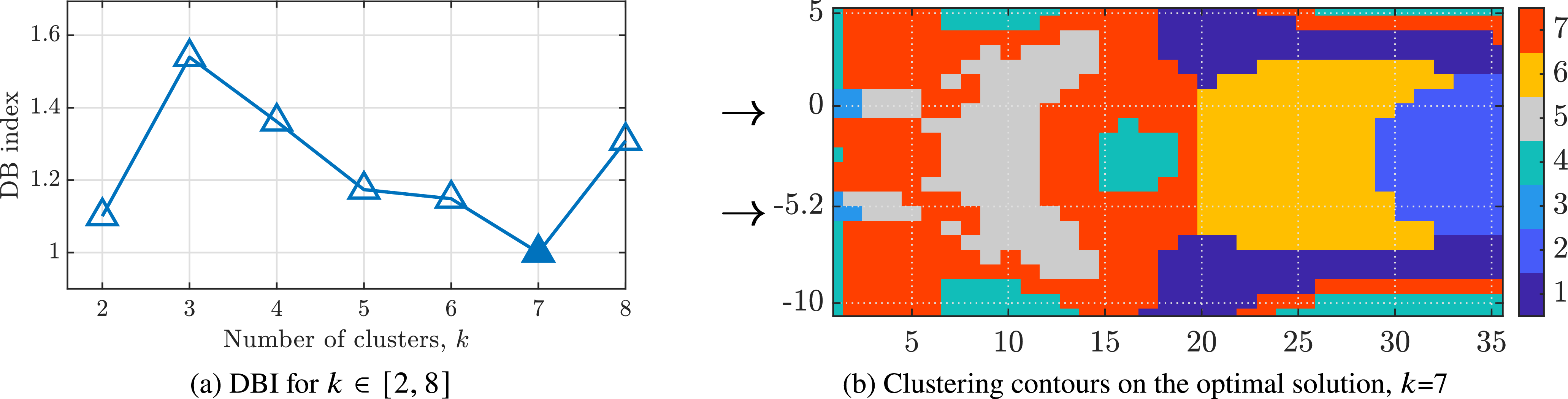
, are evaluated. Figure 12(a) presents the corresponding DBI values, with the optimal solution at
 $k = 7$
(indicated by the lowest DBI) highlighted using a filled marker. The resulting cluster contours for the streamwise velocity component in the optimal case are shown in figure 12(b).
A more detailed analysis of the cluster solution is now conducted, focusing specifically on the region near the jet exits. Figure 13 highlights this area and marks the locations of two key flow features: jet streams and recirculation bubbles, indicated by black and blue lines, respectively. Jet streams are accurately captured by cluster
 $3$
in the immediate vicinity of the orifices and by cluster
 $5$
further downstream. Recirculation bubbles, which form between jet streams, are primarily associated with cluster
 $7$
. Identification of these coherent structures, together with the validation performed in the cylinder case (§ 3.4), provides a practical, physics-informed criterion for prioritising the clusters, rather than a fully automated ranking. After selecting
 $k=7$
using the DBI, clusters are prioritised when they contain coherent structures directly involved in the symmetry-breaking mechanism. This identifies clusters
 $3$
and
 $5$
, associated with the jet streams, and cluster
 $7$
, associated with the recirculation bubbles, as the most relevant candidates for structural sensitivity. Their relevance is subsequently assessed through the perturbation tests summarised in § 4.5 and detailed in Appendix B of the supplementary material.
(a) The DBI for the clustering results with
 $k\in {[2, 8]}$
. The optimal solution based on the DBI is highlighted with a filled marker. (b) Contours of the clusters identified for the optimal clustering, k = 7. Both panels correspond to synthetic jet flow at
 $\textit{Re} = 100$
.

Figure 12 Long description
Panel A: A line graph shows the Davies-Bouldin Index (DBI) for clustering results with the number of clusters, k, ranging from 2 to 8. The x-axis represents the number of clusters, k, and the y-axis represents the DBI index. The optimal solution based on the DBI is highlighted with a filled marker at k = 7. Panel B: A contour plot displays the clusters identified for the optimal clustering, k = 7. The x-axis and y-axis represent spatial coordinates, and different colors indicate different clusters. Both panels correspond to synthetic jet flow.
Identification of the jet streams and recirculation bubbles, black and blue lines, respectively, from the clustering solution of figure 12(b).

A future automated ranking could use cluster-wise quantities such as the leading local-PCA eigenvalue, retained reconstruction energy or integrated fluctuation kinetic energy. However, such a metric would require further validation, since energetic intensity is not necessarily equivalent to structural sensitivity.
To explore the practical implications of the identified sensitivity regions, additional simulations have been conducted with slight modifications (boundary conditions, computational domain and mesh) to the baseline set-up. These cases aim to illustrate how clustering results can guide flow control strategies, setting the basis for a more detailed study. In particular, localised perturbations in the form of point forces and passive disruptors are applied to selected clusters in order to assess their influence on the onset of symmetry breaking. The next section briefly summarises illustrative results obtained when these regions are perturbed, while full details are deferred to Appendix B of the supplementary material.
4.5. Prospective flow control as clustering application
Although, as already mentioned, the primary objective of this work is the identification of structurally sensitive regions using clustering, a secondary analysis explores the potential of these results to guide flow control strategies. The present section discusses the main trends found; detailed configurations and parametric variations are reported in Appendix B of the supplementary material.
As a prospective application of the clustering framework, targeted perturbations were applied to selected clusters to assess their influence on the onset of symmetry breaking in the flow of two synthetic jets. The geometry and numerical set-up follow the configurations presented by Muñoz & Le Clainche (Reference Muñoz and Le Clainche2022), as summarised in § 4.2, with suitable modifications to accommodate the control mechanisms. Then, two strategies are explored: point forces and disruptors. Point forces consist of localised, time-dependent body forces applied at specific locations in the flow, whereas disruptors are passive square elements introduced into the domain to modify the local flow topology through geometric obstruction. Both approaches are designed to investigate the sensitivity of the regions identified by clustering, rather than to achieve optimal control solutions.
The efficacy of the control strategies is assessed using a newly introduced indicator: the symmetry-breaking cycle (cycle
 $_b$
), which denotes the piston cycle at which the flow asymmetry becomes first clearly observable. For the destabilisation objective at
 $\textit{Re}=140$
, success is defined as achieving asymmetry within the first analysed cycles. In contrast, the stabilisation objective at
 $\textit{Re}=150$
aims to delay the onset of asymmetry beyond the original transition point, cycle
 ${_b}_{org} = 22$
. An effective strategy in this case would yield cycle
 $_b$
> cycle
 ${_b}_{org}$
, or ideally maintain a symmetric flow throughout.
Point-force perturbations were primarily used to test the sensitivity of jet-stream clusters. The main finding is that forces applied within clusters associated with the jet streams have a strong influence on the onset of symmetry breaking. In flows close to instability, such perturbations were able to either advance or delay the instability depending on their placement and orientation, confirming the high structural sensitivity of these regions. In particular, perturbations aligned with the dominant jet dynamics were found to accelerate symmetry breaking, while forces applied in neighbouring clusters produced a moderate stabilising effect. These trends, described in Appendix B of the supplementary material (see figure 16 for an overview), demonstrate that the jet-stream clusters identified by VQPCA correspond to dynamically active regions whose perturbation rapidly affects the global flow state.
Disruptors were introduced to investigate the sensitivity of the cluster associated with the recirculation bubbles between the two jets, which were found to contribute to flow stabilisation. In contrast to point forces, disruptors consistently produced a strong stabilising effect when placed within this cluster. In several cases, the onset of symmetry breaking was significantly delayed, and in the most favourable configurations the flow remained symmetric for several tens of cycles. Flow visualisations indicate that disruptors modify the shape and persistence of the recirculation bubbles, promoting a more symmetric configuration. A representative comparison of disruptor locations and their stabilising effect is provided in Appendix B (see figure 18) of the supplementary material. These results highlight the central role of the recirculation-bubble cluster in governing the symmetry-breaking instability.
5. Concluding remarks
This work introduces an efficient, low-cost approach for identifying structural sensitivity in fluid flows, with computational times typically of the order of seconds. This efficiency is achieved through a data-driven method that relies exclusively on information from the direct problem, avoiding the computational expense of adjoint-based techniques.
The core of the method lies in a clustering algorithm based on VQPCA, which partitions the flow domain using a low-dimensional representation of the system. Specifically, the method builds this space from a single temporal correlation, retaining only the dominant principal component for each cluster. This enables each cluster to be uniquely defined by its temporal behaviour, effectively partitioning the flow into dynamically coherent regions. In particular, the results suggest that small perturbations in these identified regions can trigger changes in global flow dynamics, indicating a strong link between clustering-based partitioning and structural sensitivity.
The approach is validated through the canonical case of flow past a circular cylinder, a well-established benchmark. The results are consistent with known physical structures and the method was proved robust throughout variations in sampling resolution, Reynolds number and dimensionality of the dataset, demonstrating consistency with established results in the literature.
The methodology is further tested on a more complex scenario: the interaction of two planar synthetic jets. In this case, the clustering identified dynamically meaningful regions corresponding to the jet streams and the recirculation bubbles, both of which emerged as zones of potential structural sensitivity. These insights guided a prospective secondary application: the evaluation of flow control strategies based on perturbations targeted at these clusters. Although not the main focus of this study, these tests illustrate the ability of clustering to guide the placement of perturbations to either advance or delay symmetry breaking.
In summary, the clustering-based framework presented here is both robust and computationally efficient, providing rapid insight into structural sensitivity zones of fluid dynamic problems. Beyond the cases studied, the methodology shows strong potential for more complex scenarios, including the analysis of turbulent flows, experimental datasets and integration with machine learning frameworks for real-time flow analysis and control.
Supplementary material
Supplementary material is available at http://doi.org/10.1017/flo.2026.10066.
Data availability statement
Data supporting the findings of this study are openly available by contacting the authors directly by email.
Author contributions
E.M. performed the simulations, processed and visualised the results. E.M., H.D. and J.A.M. drafted the manuscript, analysed the results and reviewed and edited the manuscript. A.P. and S.L.C. supervised the study, assisted in manuscript preparation and provided critical feedback throughout the project. All authors have read and approved the final version of the manuscript.
Funding statement
E.M., J.A.M. and S.L.C. would like to thank the Comunidad de Madrid for its support through the Call Research Grants for Young Investigators from the Universidad Politécnica de Madrid and also acknowledge the grant PID2020-114173RB-I00 funded by the Spanish Ministry of Culture and Innovation MCIN/AEI/10.13039/501100011033. H.D. and A.P. are grateful for the financial support received through the Individual Fellowship Call of Université Libre de Bruxelles (ULB) and the European Commission Grant Agreement number 801505 within the framework of the Marie Sklodowska-Curie Actions (H2020) programme. The research was sponsored by the Fédération Wallonie-Bruxelles, via ‘Actions de recherche concertées – projets avancés’ for 2022–2027.
Competing interests
The authors declare no conflict of interest.
Ethical standards
The research meets all ethical guidelines, including adherence to the legal requirements of the study country.

 Nt
 Δt
 Nx
 Ny
 Nz


 ux
 ωz

 nt
 X

 ux
 k∈[2,8]

 uy
 k∈[2,8]

 N1
 R(uy1)
 f1
 k
 PSD(PC1(k))

 ux
 uy

 ux
 Re

 φ=π/21
 φ=2π
 k∈[2,8]
 Re=100


 Open access

