


%20--%3e%3c!DOCTYPE%20svg%20PUBLIC%20'-//W3C//DTD%20SVG%201.0//EN'%20'http://www.w3.org/TR/2001/REC-SVG-20010904/DTD/svg10.dtd'%3e%3csvg%20version='1.0'%20id='Layer_1'%20xmlns='http://www.w3.org/2000/svg'%20xmlns:xlink='http://www.w3.org/1999/xlink'%20x='0px'%20y='0px'%20width='64px'%20height='64px'%20viewBox='5.5%20-3.5%2064%2064'%20enable-background='new%205.5%20-3.5%2064%2064'%20xml:space='preserve'%3e%3cg%3e%3ccircle%20fill='%23FFFFFF'%20fill-opacity='0'%20cx='37.785'%20cy='28.501'%20r='28.836'/%3e%3cpath%20fill='%23595959'%20d='M37.441-3.5c8.951,0,16.572,3.125,22.857,9.372c3.008,3.009,5.295,6.448,6.857,10.314%20c1.561,3.867,2.344,7.971,2.344,12.314c0,4.381-0.773,8.486-2.314,12.313c-1.543,3.828-3.82,7.21-6.828,10.143%20c-3.123,3.085-6.666,5.448-10.629,7.086c-3.961,1.638-8.057,2.457-12.285,2.457s-8.276-0.808-12.143-2.429%20c-3.866-1.618-7.333-3.961-10.4-7.027c-3.067-3.066-5.4-6.524-7-10.372S5.5,32.767,5.5,28.5c0-4.229,0.809-8.295,2.428-12.2%20c1.619-3.905,3.972-7.4,7.057-10.486C21.08-0.394,28.565-3.5,37.441-3.5z%20M37.557,2.272c-7.314,0-13.467,2.553-18.458,7.657%20c-2.515,2.553-4.448,5.419-5.8,8.6c-1.354,3.181-2.029,6.505-2.029,9.972c0,3.429,0.675,6.734,2.029,9.913%20c1.353,3.183,3.285,6.021,5.8,8.516c2.514,2.496,5.351,4.399,8.515,5.715c3.161,1.314,6.476,1.971,9.943,1.971%20c3.428,0,6.75-0.665,9.973-1.999c3.219-1.335,6.121-3.257,8.713-5.771c4.99-4.876,7.484-10.99,7.484-18.344%20c0-3.543-0.648-6.895-1.943-10.057c-1.293-3.162-3.18-5.98-5.654-8.458C50.984,4.844,44.795,2.272,37.557,2.272z%20M37.156,23.187%20l-4.287,2.229c-0.458-0.951-1.019-1.619-1.685-2c-0.667-0.38-1.286-0.571-1.858-0.571c-2.856,0-4.286,1.885-4.286,5.657%20c0,1.714,0.362,3.084,1.085,4.113c0.724,1.029,1.791,1.544,3.201,1.544c1.867,0,3.181-0.915,3.944-2.743l3.942,2%20c-0.838,1.563-2,2.791-3.486,3.686c-1.484,0.896-3.123,1.343-4.914,1.343c-2.857,0-5.163-0.875-6.915-2.629%20c-1.752-1.752-2.628-4.19-2.628-7.313c0-3.048,0.886-5.466,2.657-7.257c1.771-1.79,4.009-2.686,6.715-2.686%20C32.604,18.558,35.441,20.101,37.156,23.187z%20M55.613,23.187l-4.229,2.229c-0.457-0.951-1.02-1.619-1.686-2%20c-0.668-0.38-1.307-0.571-1.914-0.571c-2.857,0-4.287,1.885-4.287,5.657c0,1.714,0.363,3.084,1.086,4.113%20c0.723,1.029,1.789,1.544,3.201,1.544c1.865,0,3.18-0.915,3.941-2.743l4,2c-0.875,1.563-2.057,2.791-3.541,3.686%20c-1.486,0.896-3.105,1.343-4.857,1.343c-2.896,0-5.209-0.875-6.941-2.629c-1.736-1.752-2.602-4.19-2.602-7.313%20c0-3.048,0.885-5.466,2.658-7.257c1.77-1.79,4.008-2.686,6.713-2.686C51.117,18.558,53.938,20.101,55.613,23.187z'/%3e%3c/g%3e%3c/svg%3e)
%20--%3e%3c!DOCTYPE%20svg%20PUBLIC%20'-//W3C//DTD%20SVG%201.0//EN'%20'http://www.w3.org/TR/2001/REC-SVG-20010904/DTD/svg10.dtd'%3e%3csvg%20version='1.0'%20id='Layer_1'%20xmlns='http://www.w3.org/2000/svg'%20xmlns:xlink='http://www.w3.org/1999/xlink'%20x='0px'%20y='0px'%20width='64px'%20height='64px'%20viewBox='5.5%20-3.5%2064%2064'%20enable-background='new%205.5%20-3.5%2064%2064'%20xml:space='preserve'%3e%3cg%3e%3ccircle%20fill='%23FFFFFF'%20fill-opacity='0'%20cx='37.637'%20cy='28.806'%20r='28.276'/%3e%3cg%3e%3cpath%20fill='%23595959'%20d='M37.443-3.5c8.988,0,16.57,3.085,22.742,9.257C66.393,11.967,69.5,19.548,69.5,28.5c0,8.991-3.049,16.476-9.145,22.456%20C53.879,57.319,46.242,60.5,37.443,60.5c-8.649,0-16.153-3.144-22.514-9.43C8.644,44.784,5.5,37.262,5.5,28.5%20c0-8.761,3.144-16.342,9.429-22.742C21.101-0.415,28.604-3.5,37.443-3.5z%20M37.557,2.272c-7.276,0-13.428,2.553-18.457,7.657%20c-5.22,5.334-7.829,11.525-7.829,18.572c0,7.086,2.59,13.22,7.77,18.398c5.181,5.182,11.352,7.771,18.514,7.771%20c7.123,0,13.334-2.607,18.629-7.828c5.029-4.838,7.543-10.952,7.543-18.343c0-7.276-2.553-13.465-7.656-18.571%20C50.967,4.824,44.795,2.272,37.557,2.272z%20M46.129,20.557v13.085h-3.656v15.542h-9.944V33.643h-3.656V20.557%20c0-0.572,0.2-1.057,0.599-1.457c0.401-0.399,0.887-0.6,1.457-0.6h13.144c0.533,0,1.01,0.2,1.428,0.6%20C45.918,19.5,46.129,19.986,46.129,20.557z%20M33.042,12.329c0-3.008,1.485-4.514,4.458-4.514s4.457,1.504,4.457,4.514%20c0,2.971-1.486,4.457-4.457,4.457S33.042,15.3,33.042,12.329z'/%3e%3c/g%3e%3c/g%3e%3c/svg%3e)
1. Methods and tools
1.1. Irregular grid of CLOUDY models
We compute a grid of 3,500,000 photoionization models for H ii regions using the multi-purpose photoionization code CLOUDY in its version 17.03. The input space-parameter is of dimension 13: log(U), O/H, N/O, C/O, Ne/O, S/O, Ar/O, ionizing cluster age, shape-factor, hydrogen density, optical depth, dust content, filling factor. The ionizing SED is defined by BPASS binary-including library (Eldridge et al. Reference Eldridge, Stanway, Xiao, McClelland, Taylor, Ng, Greis and Bray2017; Stanway & Eldridge Reference Stanway and Eldridge2018). For extremely large grids, we adopt a practical approach involving using randomly-distributed independent parameters, which offers an efficient way to populate datasets to train ML algorithms. The models are stored under reference HII_24 in 3MdB_17, which is a large database of photoionization models, with public access through the mySQL protocol since 2014 (http://3mdb.astro.unam.mx, see Morisset et al. Reference Morisset, Delgado-Inglada and Flores-Fajardo2015).
1.2. CLOUDY emulator using ANN
A subset of 800,000 models is defined to train the ANN. The ANN is implemented through the Tensorflow python library (http://tensorflow.org). The ANN of the 256-512-256 GELU neurons (Hendrycks & Gimpel Reference Hendrycks and Gimpel2016) takes 13 input parameters and predicts 14 emission line ratios + electron temperature + H
 $\alpha$
absolute luminosity. The training time is 2 hours on a standard GPU. The ANN allows us to generate 1 million models in 0.2 seconds (!). The ANN and the first results are described in paper I (Morisset et al. Reference Morisset, Charlot, Sánchez, Espinosa-Ponce, Barat and Dautremer2025) : https://ui.adsabs.harvard.edu/abs/2025MNRAS.538.1884M
2. Some results
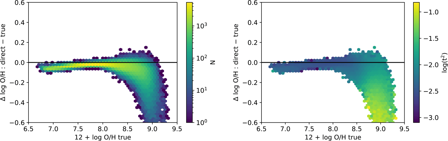
250,000 galaxy models are produced containing between 100 and 3000 H ii regions each. Global DIG emission and dust attenuation (individually defined for each H ii region) are taken into account. In Fig. 1 we show that the direct-method determination of O/H in metal-rich H ii regions and galaxies can strongly underestimate the true value. This is due to the combination of: 1) the contamination of [O
 $\,$
iii]
 $\lambda$
4363 by recombination, 2) the natural electron temperature gradient in cold regions, described by Stasińska (Reference Stasińska2005), and 3) the effect of phosphorescence contamination of [O
 $\,$
iii]
 $\lambda$
4363, see Morisset et al. in prep.
Distribution of the logarithmic difference between O/H derived from the direct method and true, H
 $\alpha$
-weighted O/H as a function of 12 + log (O/H), for the subset of 207 750 composite star-forming galaxies with log([O
 $\,$
iii]
 $\lambda$
4363/H
 $\beta$
)
 $\gt -3$
. Left: Colour-coded as a function of model number density. Right: Colour-coded as a function of root-mean-square t of H II-region temperature fluctuations. Taken from Morisset et al. (Reference Morisset, Delgado-Inglada and Flores-Fajardo2015).

Figure 1 Long description
Panel A: A scatter plot shows the distribution of the logarithmic difference between oxygen abundance derived from the direct method and true values as a function of 12 + log (O/H) true. The x-axis represents 12 + log O/H true, ranging from 6.5 to 9.5. The y-axis represents the difference in log O/H (direct - true), ranging from -0.6 to 0.6. The color scale indicates the number density of models, with yellow representing higher densities and purple representing lower densities. Panel B: Another scatter plot shows the same x and y axes but is color-coded as a function of the root-mean-square of H II-region temperature fluctuations. The color scale ranges from yellow (higher values) to purple (lower values). Both plots reveal a trend where the difference in log O/H (direct - true) varies with the true oxygen abundance, showing a noticeable pattern around 12 + log O/H true values of 8.5 to 9.0.
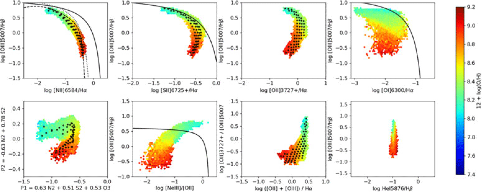
Models are compared to observations: some galaxy models are selected if they reproduce simultaneously [N ii]/H
 $\beta$
, [O
 $\,$
ii]/H
 $\beta$
, [O
 $\,$
iii]/H
 $\beta$
, and [S
 $\,$
ii]/H
 $\beta$
. He
 $\,$
i/H
 $\beta$
, and [Ar
 $\,$
iii]/H
 $\beta$
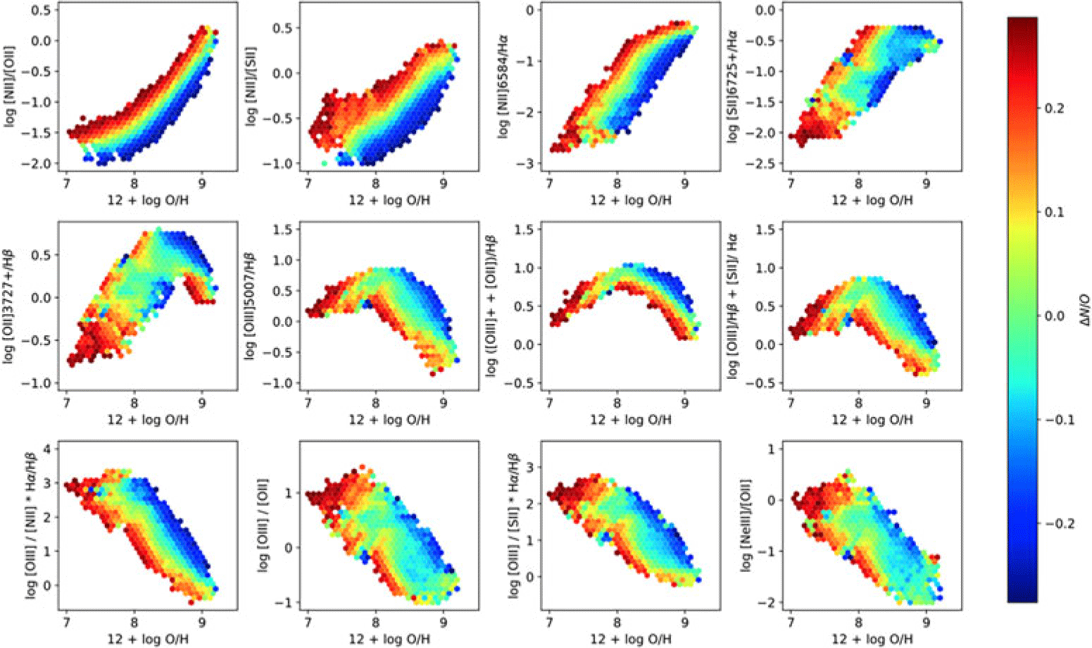
can also be used if present in the observational set. These models are shown in Fig. 2, in the case of fitting the stacked observations from Curti et al. (Reference Curti, Cresci, Mannucci, Marconi, Maiolino and Esposito2017). The selected galaxies can then be plotted in Strong Line (SL) calibrators vs. O/H diagrams. In Fig. 3 we show the effect of changing the N/O vs. O/H relationship at the level of the galaxy models. The scatter observed in the SL calibrators can be identified with real dispersions in the relationships between the different parameters, here N/O vs. O/H, but also log(U) vs. O/H, among others.
Plots for BPT-type diagrams for the results of best SF galaxies models. Black dots are from Curti et al. (Reference Curti, Cresci, Mannucci, Marconi, Maiolino and Esposito2017). Plots are taken from Morisset et al. in prep.

Strong line calibrators vs. oxygen abundance for the SF synthetic galaxies selected by fitting Curti et al. (Reference Curti, Cresci, Mannucci, Marconi, Maiolino and Esposito2017) observations. The color code follows the departure from canonical N/O vs. O/H relationship. Plots are taken from Morisset et al. in prep.

Figure 3 Long description
The image contains twelve scatter plots arranged in a 3x4 grid. Each plot shows the relationship between different emission lines and oxygen abundance (12 + log O/H) in synthetic star-forming galaxies. The color code represents the departure from the canonical N/O vs. O/H relationship, ranging from blue to red. Panel A: log [N II]/[O II] vs. 12 + log O/H. Panel B: log [N II]/[S II] vs. 12 + log O/H. Panel C: log ([N II]6584/Hα) vs. 12 + log O/H. Panel D: log ([S II]6725/Hα) vs. 12 + log O/H. Panel E: log ([O II]3727/Hβ) vs. 12 + log O/H. Panel F: log ([O III]5007/Hβ) vs. 12 + log O/H. Panel G: log ([O III] + [O II])/Hβ vs. 12 + log O/H. Panel H: log ([O III]/Hα + [S II]/Hα) vs. 12 + log O/H. Panel I: log ([O III]/Hβ) vs. 12 + log O/H. Panel J: log ([O III]/[O II]) vs. 12 + log O/H. Panel K: log ([S II]/[O II]) vs. 12 + log O/H. Panel L: log ([N II]/[O II]) vs. 12 + log O/H.
3. Conclusions and future work
ANN is a powerful tool to create very fast CLOUDY ersatz. Synthetic galaxy models obtained by summing individual H ii region models allow us to explore the effects of parameter scatters. Stay tuned for paper II. The ANN can also be used for any massive production of H ii region models, e.g. in an MCMC method or a Genetic algorithm, to derive physical/chemical parameters from observed line ratios. The results will soon be updated using a grid of models using new CLOUDY c25.00.
Acknowledgments
The initial stages of this work were conceived and developed during a CM sabbatical at the Institut d’Astrophysique de Paris (IAP) to collaborate with SC. CM gratefully acknowledges the PASPA grant that supported this sabbatical. CM acknowledges the support of UNAM/DGAPA/PAPIIT grants IN101220 and IG101223.
 α

 λ
 β
 >−3

 Open access

