1 Introduction
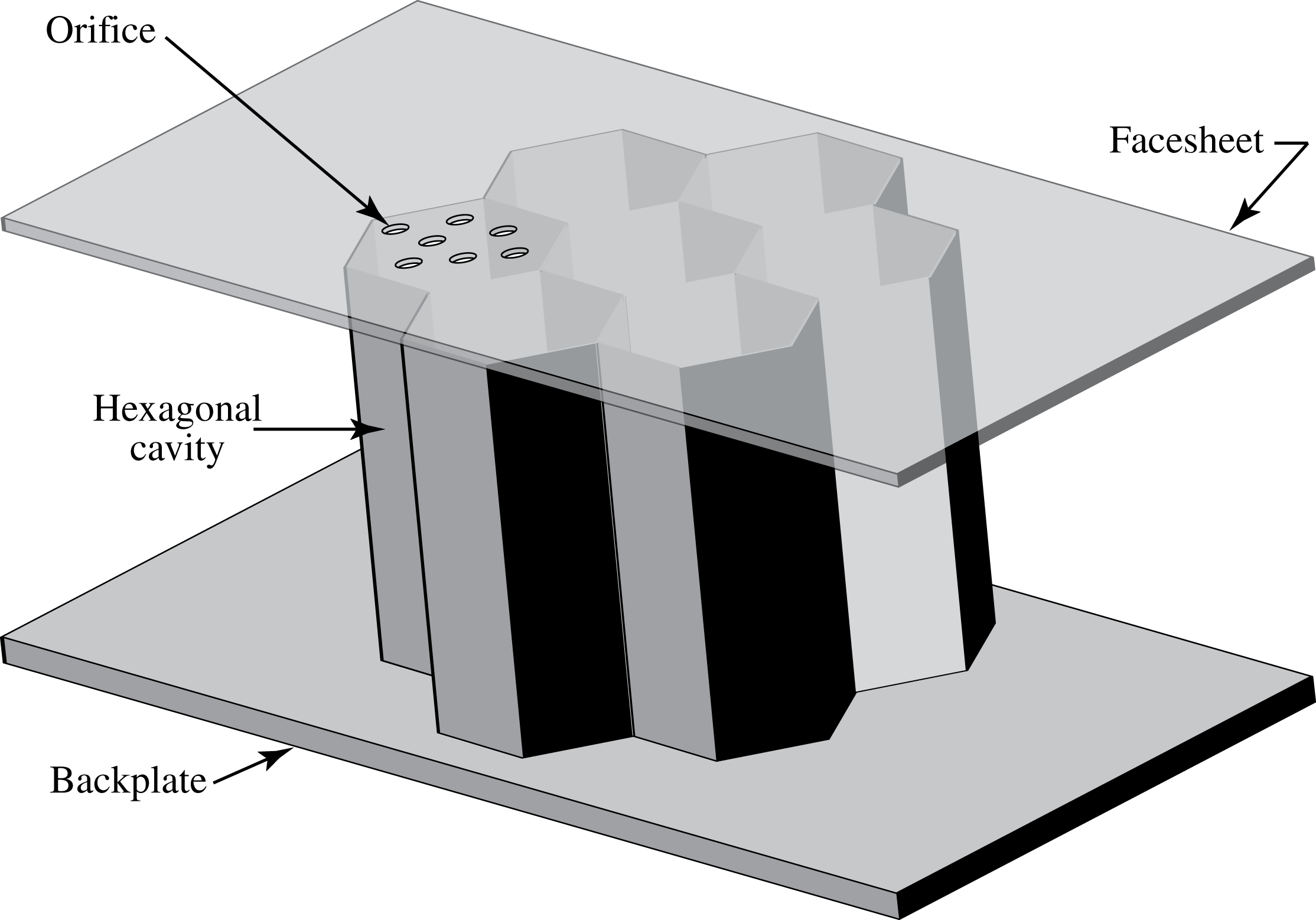
Acoustic liners are an important component of aircraft noise reduction for internal engine flow paths to reduce fan, compressor, turbine and jet noise (Motsinger & Kraft Reference Motsinger, Kraft and Hubbard1995). They work by converting energy bound to the acoustic field into vorticity-bound energy to lower the sound amplitude. Several classes of liners of varying complexity are available with designable sound absorption characteristics. For example, backing cavities can be added to small, sharp-edged openings to tune the frequency response of the liner’s acoustic absorption to the application of interest. A schematic of a single degree-of-freedom liner is shown in figure 1 where the facesheet containing the orifices is fixed to an array of closed hexagonal cavities; all structural elements are assumed to be rigid.
Schematic of a single degree-of-freedom conventional acoustic liner.

For typical aircraft applications, the wavelength of sound to be attenuated by the liner is much larger than the characteristic dimensions of the liner orifice and its cavity depth and a ‘lumped element’ method of analysis has proven useful. For conventional liners, such as the one shown in figure 1, the unit element is a Helmholtz resonator whose dynamics are widely known (Morse & Ingard Reference Morse and Ingard1968; Pierce Reference Pierce1994) for low-amplitude, single frequency, incident sound waves in an otherwise still environment. In the lumped element context the resonator alters the incident sound field by (1) generating vorticity at the orifice side walls through the no-slip boundary condition and (2) scattering a portion of the incident sound field into a cylindrical (if in two dimensions) or spherical acoustic field. Correlations exist to connect the physical dimensions of the resonator to its characteristic response that are usually based on approximate solutions to account for viscosity and/or the scattered pressure field; for example, the resonant frequency is
 $$\begin{eqnarray}{\it\omega}_{H}=c_{\infty }\left(\frac{A}{\ell ^{\prime }V}\right)^{1/2}\end{eqnarray}$$
for a resonator with orifice area
 $A$
, cavity volume
 $V$
, orifice ‘neck’ length
 $\ell ^{\prime }=\ell +2{\rm\Delta}\ell$
, operating in an environment with speed of sound
 $c_{\infty }$
. The geometrical neck length
 $\ell$
is modified by a correction
 ${\rm\Delta}\ell \approx 0.8\sqrt{A/{\rm\pi}}$
that accounts for the scattered pressure field and its influence on the effective mass of the air near the orifice.
At the conditions for which (1.1) is valid, the resonator dynamics can be accurately described by linear equations with constant coefficients. Under these conditions the interaction of an incident sound wave with the resonator can be described in the temporal frequency domain where the concept of an acoustic impedance, with symbol
 $Z$
, is useful. For a surface with local outward unit normal
 $\boldsymbol{n}$
, the acoustic impedance is defined as
 $$\begin{eqnarray}Z=\frac{\hat{p}}{\hat{\boldsymbol{v}}\boldsymbol{\cdot }\boldsymbol{n}},\end{eqnarray}$$
where
 $\hat{p}$
and
 $\hat{\boldsymbol{v}}$
are the Fourier coefficients of the unsteady acoustic pressure and velocity fields on the surface, respectively. It is clear that
 $Z$
is frequency dependent and complex valued, taking on the values of 0,
 $\infty$
and
 ${\it\rho}_{\infty }c_{\infty }$
for ‘pressure release’, hard wall and boundary-free planar propagation through a uniform atmosphere. It can be shown that if
 $Z$
is prescribed on a surface then a Neumann boundary condition results that makes the acoustic problem well posed (Evans Reference Evans1998), at least for frequency domain problems. When used in conjunction with time-domain problems, care must be taken to ensure well posedness (Tam & Auriault Reference Tam and Auriault1996). It is to be stressed that the impedance
 $Z$
is an effective boundary condition used to hide the complexity of the fundamental flow physics involved in the interaction of sound in a compressible viscous gas with a perforated, cavity-backed surface. It is not a general physical property of the medium but depends instead on the particular physical scenario and on how the impedance is ‘educed’.
Because, in large part, Helmholtz resonators are the unit element in conventional acoustic liners, a liner is usually described by its acoustic impedance which, under suitable conditions, provides a rational means to quantify and, ultimately, design liners for use in acoustic attention. However, typical aircraft conditions are far from the linear regime in which an acoustic impedance is natural. For example, laminar or turbulent grazing flows are present, the sound amplitude is not ‘small’, and the multiple orifices (see figure 1) can interact because of their close proximity. These complexities must be embedded within the liner’s acoustic impedance
 $Z$
and create a large possible parametric dependence to capture these effects, as discussed in the survey by Motsinger & Kraft (Reference Motsinger, Kraft and Hubbard1995), creating a complex modelling challenge. Proposed future applications of acoustic liners to aircraft exteriors will further increase the parametric range required of impedance models (Posey, Tinetti & Dunn Reference Posey, Tinetti and Dunn2006).
It is even questionable whether the reliance on the acoustic impedance is itself useful at nonlinear conditions since the fundamental concept lies in the frequency domain where single frequency behaviour gives way to multiple (tonal) frequency and/or broadband behaviour, depending the level of nonlinearlity and specific flow scenario. A time-domain approach to liners may yield an easier modelling approach, as in prior work (Zhang & Bodony Reference Zhang and Bodony2012), but the historical inertia of acoustic impedance is likely to remain. The purpose of this work is to begin developing an accurate database of the orifice–sound–flow interaction to improve liner modelling and design at realistic conditions.
1.1 Literature review
The preceding discussion builds upon existing and on-going work to characterize the performance of acoustic liners or Helmholtz resonators in complex conditions, such as with significant grazing flow and/or at nonlinear conditions. Early work by Sivian (Reference Sivian1935) to examine small-orifice impedance was expanded by Ingard & Labate (Reference Ingard and Labate1950) who observed that the size of the orifice could significantly change the sound-induced flow inside the orifice due to viscosity, possibly generating an oscillatory turbulent jet, and displaying a nonlinear impedance. Rogers & Hersh (Reference Rogers and Hersh1975) and Hersh & Rogers (Reference Hersh and Rogers1976) used a single orifice mounted within a water tunnel to visualize the oscillatory flow to develop a semi-empirical impedance model that accounted for high-amplitude conditions.
More recent experiments on the fluid mechanics of liners emphasized more the detailed flow structure. Hughes & Dowling (Reference Hughes and Dowling1990) and Dowling & Hughes (Reference Dowling and Hughes1992) studied in detail the vortex shedding of screens with regular arrays of slits and circular perforations with mean bias flow, respectively. Building on the work of Howe (Reference Howe1979), Eldredge & Dowling (Reference Eldredge and Dowling2003) considered the effectiveness of a cylindrical perforated liner with mean bias flow in its absorption. Ozalp, Pinarbasi & Rockwell (Reference Ozalp, Pinarbasi and Rockwell2003) studied the self-excited oscillations of a turbulent boundary layer along a perforated plate closed by a cavity using particle image velocimetry (PIV). Ma, Slaboch & Morris (Reference Ma, Slaboch and Morris2009) also investigated the detailed fluid dynamic characteristics of a flow-excited Helmholtz resonator using PIV and proposed a predictive methodology for the corresponding measurements. Marx & Aurégan (Reference Marx and Aurégan2013) performed linear stability normal mode analysis of a lined wall with flow and the effect of viscous dissipation while Fischer, Bake & Bassetti (Reference Fischer, Bake and Bassetti2013) performed a comparison between the PIV and computational aeroacoustic results in the vicinity of an acoustic liner, with phase-locked results, with encouraging agreement between a linearized boundary condition and the experimental data. A recent theoretical nonlinear Helmholtz model was developed by Singh & Rienstra (Reference Singh and Rienstra2014) to be applicability in the weakly nonlinear sound amplitude regime. Ćosić et al. (Reference Ćosić, Wassmer, Terhaar and Paschereit2015) investigated the effect of hot grazing flow over a Helmholtz resonator using PIV.
The use of acoustic impedance to characterize liner performance has inspired a long history of investigation to develop the measurement and eduction tools necessary to deduce it. For example, through extensive experiments Melling (Reference Melling1973) determined the impedance of a liner by applying a semi-empirical method and realized that the linear or nonlinear behaviour of the excited flow in the liner depended mostly on the incident sound pressure level (SPL). The popular two-microphone method for impedance eduction, such as used by Dean (Reference Dean1974), was used because of its simplicity and reliability, even when a grazing flow was present. Solving an associated inverse problem is an indirect way to educe the impedance and has been studied by several, including Jones et al. (Reference Jones, Tracy, Watson and Parrott2002), Taktak et al. (Reference Taktak, Ville, Haddar, Gabard and Foucart2010), Enghardt et al. (Reference Enghardt, Fisher, Schulz and Busse-Gerstengarbe2012) and Piot, Primus & Simon (Reference Piot, Primus and Simon2012). For full-scale engines, an insertion loss method can be used (Motsinger & Kraft Reference Motsinger, Kraft and Hubbard1995). Schuster (Reference Schuster2012) recently discussed the effect of different ensemble averaging approaches when using an in situ two-microphone method in the presence of a turbulent grazing flow.
Modelling the acoustic impedance enables liner design and optimization, often in a semi-empirical approach, by emphasizing the flow physics rather than providing purely parametric models. Hersh & Rogers (Reference Hersh and Rogers1976) were among the first to develop a fluid mechanical model to predict orifice resistance and reactance as a function of incident sound pressure level, frequency and orifice geometry. Howe (Reference Howe1979) developed an expression for the Rayleigh conductivity of an aperture through which a high-Reynolds-number flow passed, whereas Cummings (Reference Cummings1987) established a relation between the acoustic resistance and the discharge coefficient via a quasi-steady model. A nonlinear discrete vortex dynamic model was proposed by Jing et al. (Reference Jing, Sun, Wu and Meng2001) and followed by experiments of low-Mach turbulent boundary layers over a perforated facesheet. The model was then studied in more detail by Sun et al. (Reference Sun, Jing, Zhang and Shi2002) who investigated a similar case but focused on the interaction of the bias and grazing flow effect with an empirical equation connecting the acoustic impedance with the grazing flow Mach number and the effective discharge coefficient. Hersh, Walker & Celano (Reference Hersh, Walker and Celano2003) developed a time-domain model to predict the impedance with a particular emphasis on nonlinearity and discharge coefficient relationship while Kooijman, Hirschberg & Golliard (Reference Kooijman, Hirschberg and Golliard2008) investigated the acoustical response of orifices under different boundary-layer profiles and liner edge geometries. More specific models regarding the interaction effect of perforated plates with bias flow can be found in Lee, Ih & Peat (Reference Lee, Ih and Peat2007). Tonon, Moers & Hirschberg (Reference Tonon, Moers and Hirschberg2013) extensively investigated the inflow vena contracta, a parameter strongly related to the inflow discharge coefficient, and obtained a semi-empirical correction model for a two-dimensional wall perforation. Scarpato et al. (Reference Scarpato, Tran, Ducruix and Schuller2012) and Scarpato, Ducruix & Schuller (Reference Scarpato, Ducruix and Schuller2013) performed extensive work on modelling the acoustic properties of perforate backed by a cavity with bias flow at low Strouhal number. Zhou & Bodén (Reference Zhou and Bodén2014) investigated the bias flow under medium and high-level acoustic excitation and found more complex acoustic properties compared with the no-bias flow case.
The usually small geometry (orifice diameters are of the order of 1 mm) and complex flow field have prompted several computational studies to examine the detailed flow within the resonator/liner region and, in later work, to directly estimate the impedance. Initial efforts focused on slit geometries that were computationally less demanding and gradually increased the flow complexity from normal incidence, no grazing flow (Tam et al. Reference Tam, Kurbatskii, Ahuja and Gaeta2001) to those with a grazing flow (Tam, Ju & Walker Reference Tam, Ju and Walker2008b ; Zhang & Bodony Reference Zhang and Bodony2011). More recently, fully three-dimensional numerical simulations of sound interacting with resonators have been performed with different geometries. Tam et al. (Reference Tam, Ju, Jones, Watson and Parrott2008a ) observed the formation of vortex rings in their simulations of a rectangular orifice liner and noted that their earlier results from slit liners had a very different flow topology, a result confirmed by Roche et al. (Reference Roche, Leylekian, Delattre and Vuillot2009). Xu, Li & Guo (Reference Xu, Li and Guo2014) extended earlier slit liner simulations into a fully three-dimensional simulation and found the absorption coefficients agreed very well with the previous two-dimensional simulations. An example application of alternative numerical methods (i.e. the lattice Boltzmann method) to liner investigations can be found in Ji & Zhao (Reference Ji and Zhao2014).
Recent work by Tam et al. (Reference Tam, Pastouchenko, Jones and Watson2014) focused on creating a two-dimensional model of the NASA Langley grazing flow impedance tube (GFIT) fitted with an eight-orifice slit liner. Care was taken to match, as much as possible, the spatially developing flow within the GFIT through a tuned eddy viscosity and grazing acoustic incidence along the duct; in addition, a slit liner was manufactured to match the computational model. Comparisons between the experimental and computational efforts identified the importance of the GFIT acoustic termination conditions at low-frequency conditions while suggesting that liners can add drag, of the order of 4 %, for a liner with approximately 10 % porosity. Furthermore, impedance predictions by the simulations using the same data reduction method as used with the experimental data exhibited the same frequency dependence as did the experimental data but quantitative differences existed in the resistance and reactance at low frequencies, perhaps due to differences in modelling the GFIT termination impedance. Predictions at higher frequencies were, in general, in closer quantitative agreement between the two methods.
1.2 Objective of the present study
Prior work on the behaviour of acoustic liners and/or Helmholtz resonators has not addressed several fundamental questions, including (1) how does a turbulent grazing flow interact with a cavity-backed orifice in the presence of an incident acoustic field and (2) how can reduced-order models be constructed to account for this interaction? Our earlier work using direct numerical simulations for examining the flow in and around a hexagonal cavity-backed circular orifice did not include any grazing flow but showed, among other things, how the fully three-dimensional flow, possibly turbulent, generated by the acoustic field can modify the acoustic impedance and how to model this interaction to predict the change in the impedance (Zhang & Bodony Reference Zhang and Bodony2012). The present work extends our simulation database and analysis to include laminar and turbulent grazing flows using acoustic fields and liner geometries that are relevant to those used at NASA and industry.
The results of this work are presented as follows. We examine first the essential hydrodynamic elements of the interactions followed by the acoustic impedance and its reduced-order modelling. We start by presenting the computational model derived from the NASA Langley GFIT facility and briefly discussing verification. Subsequently, a global visualization of the flow in and around the orifice is presented prior to quantifying the flow near the orifice, estimating the discharge coefficient and relevant pressure statistics and assessing the liner drag. Attention is paid to how to effectively scale the data.
2 Computational model
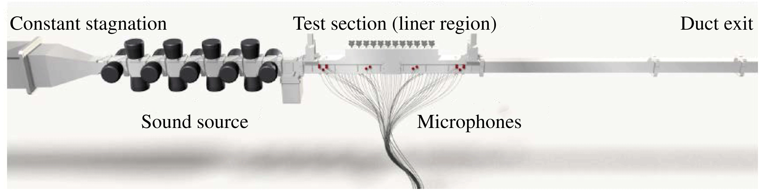
The computational model is derived from the NASA Langley grazing flow impedance tube (GFIT), as shown in figure 2. The GFIT test section is rectangular with dimensions
 $2^{\prime \prime }\times 2.5^{\prime \prime }$
and is located downstream of a speaker driver bank and high-pressure plenum. Within the test section, whose axial location may be adjusted, the liner sample is installed on one side of the duct while several pressure microphones are mounted on the opposite (hardwall) side of the duct. Downstream of the test section the duct continues into a vacuum termination. A Pitot probe is available for making streamwise velocity surveys at several locations within the duct, and the test section location is chosen to, in part, set the desired boundary-layer thickness at the liner sample upstream edge. The grazing flow Mach number can be controlled up to Mach 0.6. Additional details on the GFIT and its data acquisition system are available in Jones & Watson (Reference Jones and Watson2011). M. G. Jones & W. R. Watson (2012, private communication) provided a baseline experimental dataset based on a Mach 0.5 grazing flow over a single degree-of-freedom conventional liner (liner details will be presented later) that included Pitot profiles at locations away from the test liner and impedance values taken under single frequency, 130 dB conditions.
Grazing Flow Impedance Tube (GFIT) at NASA Langley Research Center. Image courtesy Dr Michael Jones, NASA Langley.

2.1 RANS-based duct flow simulation
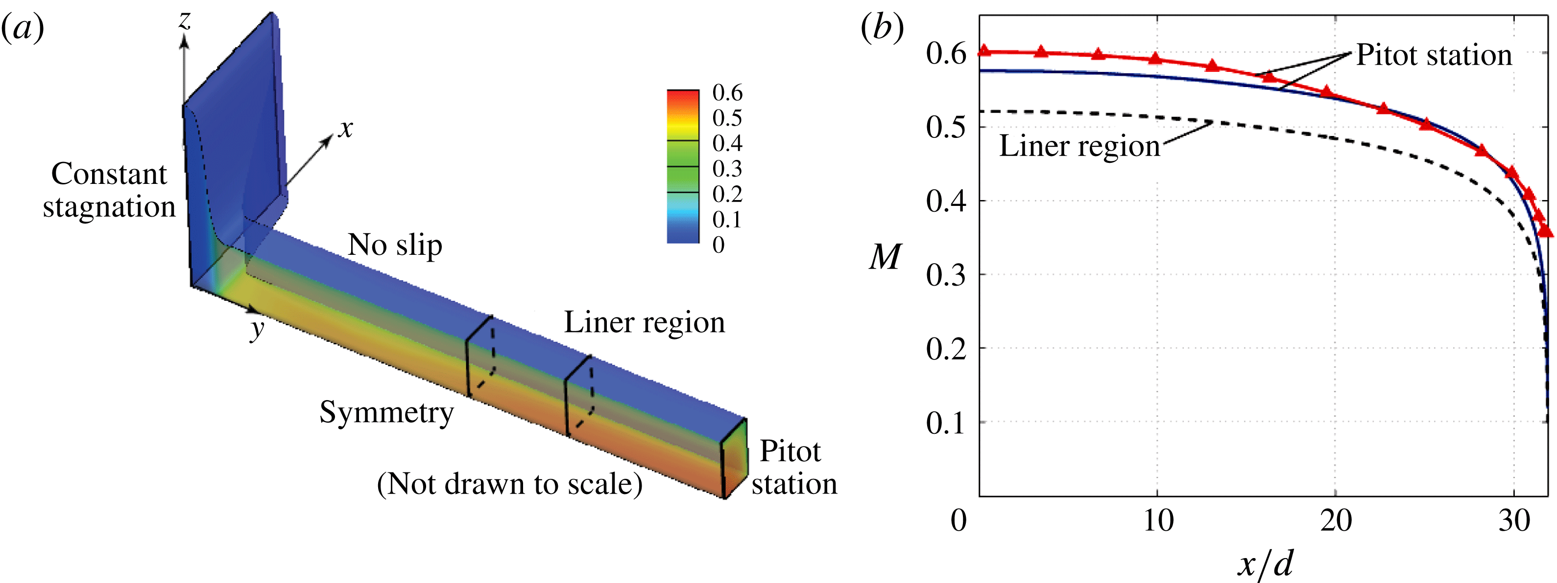
The Pitot data available within the GFIT is sufficient to estimate a large portion of the grazing flow profile but several additional parameters are needed from which to construct a viable computational model. To provide additional parameter estimates, a Reynolds-averaged Navier–Stokes (RANS) simulation was conducted of a large portion of the GFIT, including the upstream plenum and a significant portion of the exit ductwork. The NASA-provided CAD files were used to construct a structured grid on which the commercial CFD package Fluent was used to simulate the steady flow within the GFIT using the standard
 $k$
–
 ${\it\epsilon}$
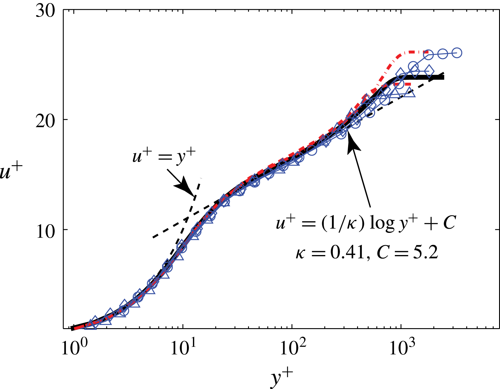
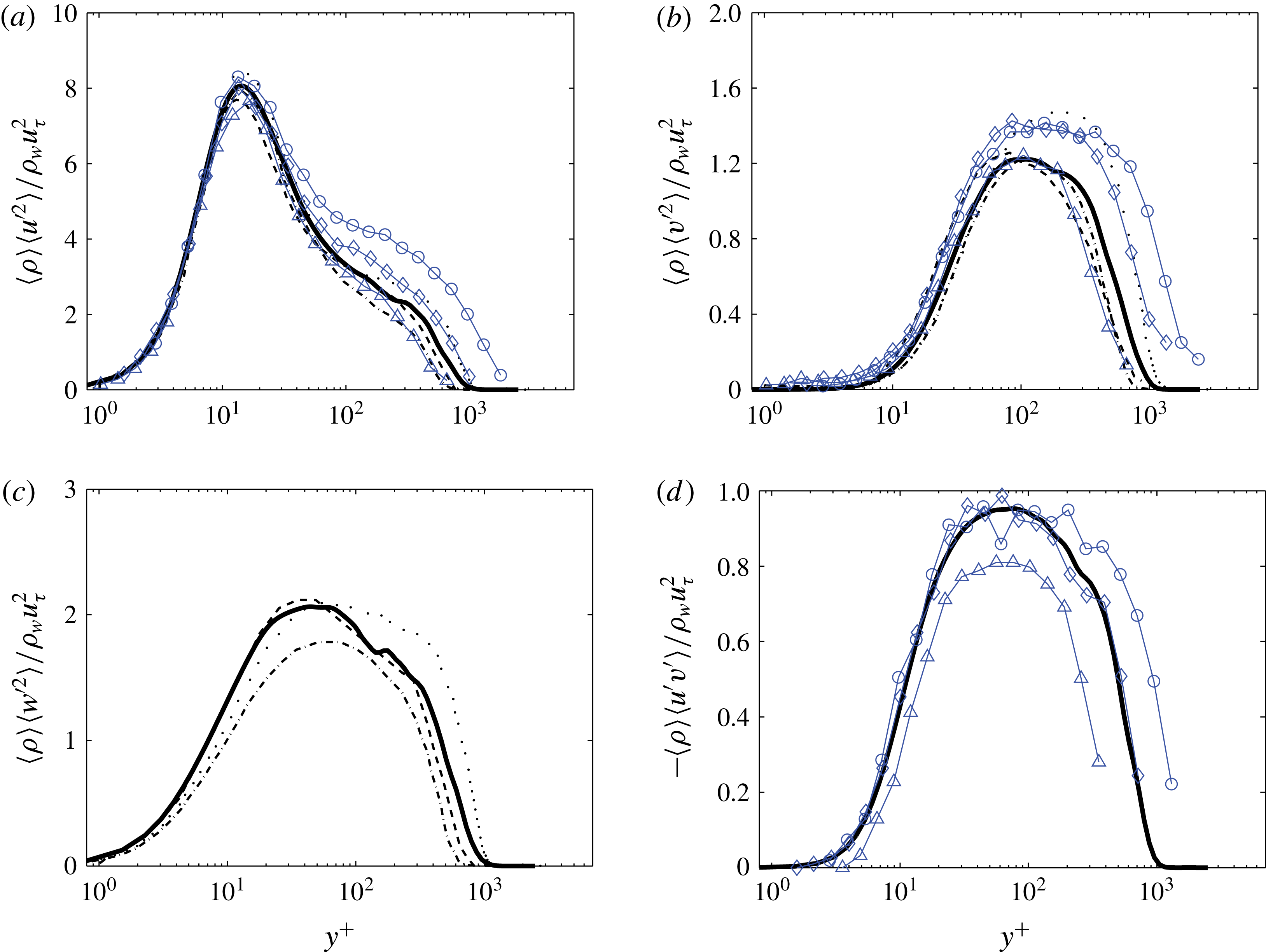
turbulence model. Only hardwall conditions were used in the RANS prediction with adiabatic thermal conditions and the rectangular symmetry of the tunnel was used to reduce the grid requirements by using symmetry plane boundary conditions. The known plenum pressure and atmospheric temperature were used to estimate the total pressure and total temperature coming into the plenum, while the exit pressure and laminar-to-turbulent transition location were adjusted until the predicted and measured velocity profiles matched to a reasonable degree, as shown in figure 3. At the Pitot location the local Mach number was approximately 0.6 while at the liner location it was closer to Mach 0.5. As table 1 shows, several parameters were estimated from both experimental and simulation datasets and found to have differences less than 10 %. Other than to ensure grid convergence, no attempts were made to assess the sensitivity of the RANS predictions to the particular model chosen; the present results are similar to those found in Tam et al. (Reference Tam, Pastouchenko, Jones and Watson2014) using an entirely different method.
The RANS results provide confidence that the basic thermodynamic state and flow field throughout the GFIT are sufficiently characterized to permit the detailed direct numerical simulations to proceed. However, they also show that the Reynolds number based on the momentum thickness is approximately 23 000 at the liner test section, which is too large for a direct numerical simulation to be viable. Because prior experiments (Goldman & Panton Reference Goldman and Panton1976) suggest that the ratio of the momentum thickness
 ${\it\delta}^{\dagger }$
to the orifice diameter
 $d$
is an important parameter, it was decided to artificially lower the Reynolds number to
 $Re_{{\it\delta}^{\dagger }}\approx 2300$
while keeping the ratio
 ${\it\delta}^{\dagger }/d$
and the Mach number fixed at 2.0 and 0.5, respectively. The consequence of this modelling assumption is that the energy in the scales of motion smaller than the orifice diameter are reduced. However, in wall units for the reduced Reynolds numbers, the orifice diameter is
 $d^{+}\approx 114\gg 1$
so that it is reasonable to assume that only the larger scales of motion within the turbulent boundary layer are able to effectively interact with the orifice, and that smaller-scale motions are dynamically unimportant. There are not currently means to perform a posteriori tests on this modelling assumption.
Velocity profile comparison between the experimental data and simulation results. Legend: ——, simulation data at the exit of the plane of the duct; –▵–, experimental data at the exit plane of the duct; - - - -, simulation data at the centre of the test section of the duct.

Comparisons of the turbulent boundary-layer features between the simulation results and experimental data.

2.2 Geometric model
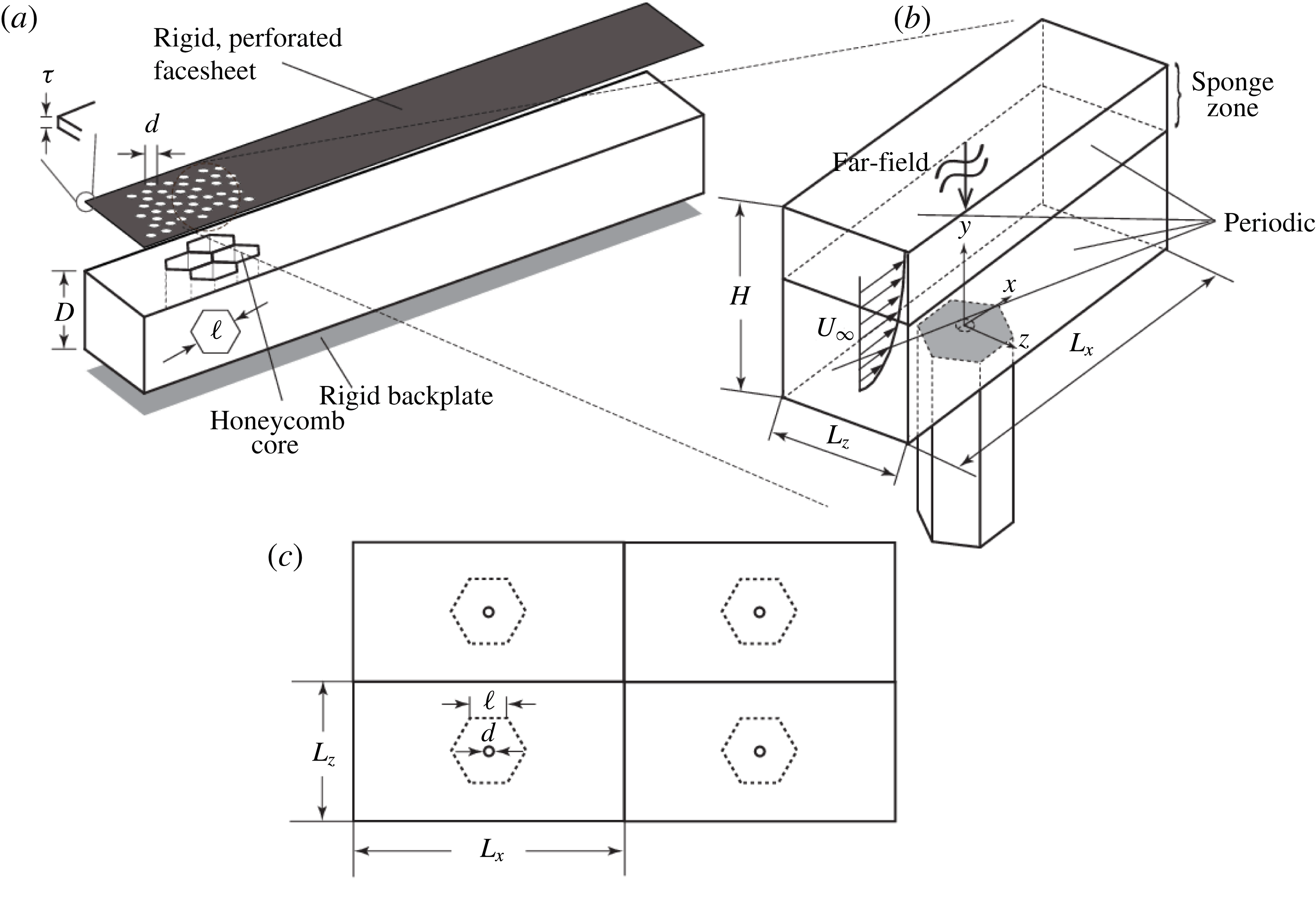
The liner geometry tested within the GFIT has a facesheet thickness of
 ${\it\tau}=0.64$
mm (refer to figure 4(a) for symbol definitions), an orifice diameter of
 $d=0.99$
mm, a cavity depth of
 $D=38.1$
mm and a cavity width of
 $\ell =5.49$
mm. The open-area porosity is 8.7 % which corresponds to, on average, 8–9 orifices per cavity; the spacing of the orifices is not centred over the cavities so, at times, an orifice may span two or three cavities and thus be partially blocked by the cavity side walls. Simplification of the geometry was used to reduce the computational cost by including only one orifice per cavity and increasing the inter-orifice spacing so as to reduce their interaction. The resulting geometry is shown in figure 4(b) where the streamwise and spanwise lengths of the exterior domain,
 $L_{x}\approx 240d$
and
 $L_{z}\approx 80d$
, respectively, result in an assumed periodicity of the liner as shown in figure 4(c). Reducing the orifice-per-cavity count from 8–9 to 1 reduces the effective open-area porosity to 0.99 %. Finally, note that the present simulations use a temporally evolving boundary-layer model where the thickness of the layer grows with time rather than in the downstream direction. Consequences of these modelling assumptions will be discussed later in this paper.
Several views of the computational model. (a) Important liner dimensions (adapted from Zhang & Bodony (Reference Zhang and Bodony2012)); (b) single liner with isolated orifice under a grazing flow; and (c) assumed periodicity.

2.3 Grid design
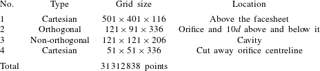
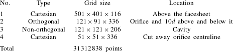
As noted in § 1, the simulations include a turbulent boundary layer grazing a circular orifice with a hexagonal backing cavity in the presence of an externally imposed incident acoustic field. The liner geometry is identical to that used previously (Zhang & Bodony Reference Zhang and Bodony2012) without a grazing flow but with an enlarged domain above the liner facesheet. Four meshes are arranged in an overset – sometimes called Chimera – setting where multiple grids can overlap and their common information is communicated by interpolation (Bodony et al.
Reference Bodony, Zagaris, Reichert and Zhang2011; Reichert, Heath & Bodony Reference Reichert, Heath and Bodony2012). Details about the individual grids are given in table 2 where grid 1 is used to hold the turbulent boundary layer while grids 2–4 are primarily to represent the circular orifice and its backing cavity. The individual grids are relatively simple to generate while their interpolation data was determined using a NASA-developed pre-processing tool (Suhs, Rogers & Dietz Reference Suhs, Rogers and Dietz2003) coupled to one developed at the Air Force Research Laboratory to produce sixth-order interpolation stencils (Sherer, Visbal & Galbraith Reference Sherer, Visbal and Galbraith2006). The minimum grid spacing in the orifice is
 ${\rm\Delta}r_{min}=0.0075d$
at the orifice walls. In the
 $z$
-direction, a uniform grid spacing
 ${\rm\Delta}z_{min}=0.01d$
is used
 $1d$
offset above and below the orifice. At
 $10d$
away from the orifice, the resolution decreases smoothly but ensures
 ${\rm\Delta}z_{min}\leqslant 0.1d$
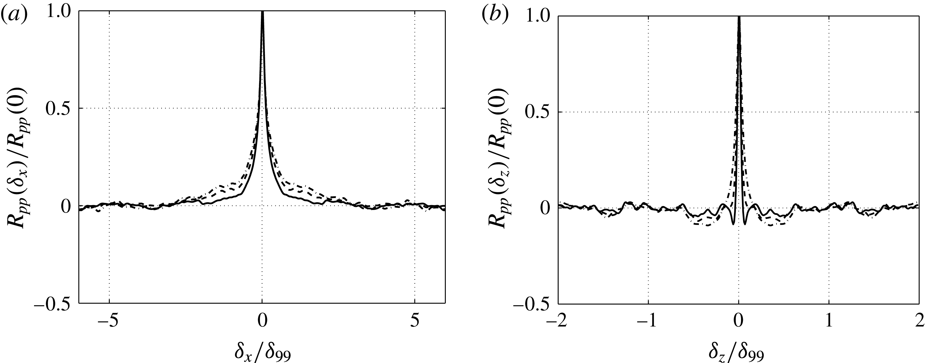
. Also note that the size of the upper rectangular box is set to be sufficiently large for fully uncorrelated statistics, as noted in appendix A. The in-orifice flow has been shown to be fully resolved in prior work (Zhang & Bodony Reference Zhang and Bodony2012).
Grid information used in the numerical simulation.
2.4 Numerical method
On each of the four grids we solve the compressible Navier–Stokes equations in a non-orthogonal coordinate system
 ${\bf\xi}={\it\bf\Xi}(\boldsymbol{x})$
, with
 ${\bf\xi}=({\it\xi},{\it\eta},{\it\zeta})^{\text{T}}$
, written in conservative form
 $$\begin{eqnarray}\displaystyle & \displaystyle \frac{\partial }{\partial t}\left(\frac{{\it\rho}}{J}\right)+\frac{\partial }{\partial {\it\xi}_{j}}({\it\rho}U_{j})=0 & \displaystyle\end{eqnarray}$$
 $$\begin{eqnarray}\displaystyle & \displaystyle \frac{\partial }{\partial t}\left(\frac{{\it\rho}u_{i}}{J}\right)+\frac{\partial }{\partial {\it\xi}_{j}}({\it\rho}u_{i}U_{j}+p\hat{{\it\xi}}_{j,i}-{\it\tau}_{ki}\hat{{\it\xi}}_{j,k})=0 & \displaystyle\end{eqnarray}$$
 $$\begin{eqnarray}\displaystyle & \displaystyle \frac{\partial }{\partial t}\left(\frac{{\it\rho}E}{J}\right)+\frac{\partial }{\partial {\it\xi}_{j}}(\{{\it\rho}E+p\}U_{j}-\hat{{\it\xi}}_{j,i}\{u_{k}{\it\tau}_{ik}-q_{i}\})=0, & \displaystyle\end{eqnarray}$$
 $\text{J}=|\partial \boldsymbol{x}/\partial {\bf\xi}|$
is the Jacobian of the grid transformation,
 $\hat{{\it\xi}}_{j,i}=\text{J}^{-1}\partial {\it\xi}_{j}/\partial x_{i}$
are the Jacobian-weighted metrics and
 $U_{i}=u_{j}\hat{{\it\xi}}_{i,j}$
are the contravariant velocities. A Newtonian fluid with Fourier’s law of heat conduction is assumed such that
 $$\begin{eqnarray}\displaystyle & \displaystyle {\it\tau}_{ij}={\it\mu}\left(\frac{\partial u_{i}}{\partial x_{j}}+\frac{\partial u_{j}}{\partial x_{i}}\right)+{\it\lambda}\frac{\partial u_{k}}{\partial x_{k}}{\it\delta}_{ij} & \displaystyle\end{eqnarray}$$
 $$\begin{eqnarray}\displaystyle & \displaystyle q_{i}=-k\frac{\partial T}{\partial x_{i}}, & \displaystyle\end{eqnarray}$$
 ${\it\lambda}={\it\mu}_{B}-2{\it\mu}/3$
and
 ${\it\mu}_{B}=0.6{\it\mu}$
for air. The temperature dependence of
 ${\it\mu}$
and
 $k$
are given by power laws
 $$\begin{eqnarray}\displaystyle \frac{{\it\mu}}{{\it\mu}_{\infty }}=\frac{k}{k_{\infty }}=\left(\frac{T}{T_{\infty }}\right)^{n}, & & \displaystyle\end{eqnarray}$$
with
 $n=0.666$
. When the equations are non-dimensionalized with respect to the ambient density
 ${\it\rho}_{\infty }$
, the ambient speed of sound
 $a_{\infty }$
, the orifice diameter
 $d$
and the ambient viscosity
 ${\it\mu}_{\infty }$
the equation of state for a calorically perfect ideal gas is
 $$\begin{eqnarray}\displaystyle p=\frac{{\it\gamma}-1}{{\it\gamma}}{\it\rho}T, & & \displaystyle\end{eqnarray}$$
with
 ${\it\gamma}=C_{p}/C_{v}$
, the ratio of specific heats, fixed at 1.4. The equations are discretized using a node-centred finite difference approach of the form
 $$\begin{eqnarray}\frac{\partial }{\partial {\it\xi}}\approx \unicode[STIX]{x1D64B}^{-1}\unicode[STIX]{x1D64C},\end{eqnarray}$$
where
 $\{\unicode[STIX]{x1D64B},\unicode[STIX]{x1D64C}\}$
are explicit summation-by-parts matrices (Strand Reference Strand1994) that are eighth-order accurate in the interior and fifth-order accurate globally. The required second derivatives use repeated first derivatives and do not provide dissipation for under-resolved flow scales so that a high-order spectral like filter is used to preserve numerical stability (Visbal & Gaitonde Reference Visbal and Gaitonde2002). Time integration uses the standard fourth-order Runge–Kutta method.
The boundary conditions listed in figure 4 and the no-slip, isothermal condition applied to all solid surfaces use the simultaneous-approximation-term formulation developed by Svärd, Carpenter & Nordström (Reference Svärd, Carpenter and Nordström2007) and Svärd & Nordström (Reference Svärd and Nordström2008). A ‘sponge’ zone (Bodony Reference Bodony2006) is used above the facesheet to accurately enforce the incident acoustic wave while simultaneously absorbing reflected acoustic waves. The incident acoustic field is planar, monochromatic and of the form,
 $$\begin{eqnarray}\displaystyle \boldsymbol{q}_{inc}^{\prime }(\boldsymbol{x},t)=A[1,\boldsymbol{k}/({\it\rho}_{\infty }c_{\infty }^{3}|\boldsymbol{k}|),1/c_{\infty }^{2}]^{\text{T}}\exp \{\text{i}(\boldsymbol{k}\boldsymbol{\cdot }\boldsymbol{x}-{\it\omega}t)\}, & & \displaystyle\end{eqnarray}$$
with assumed real part, where
 $\boldsymbol{q}_{inc}^{\prime }=[{\it\rho}_{inc}^{\prime },\boldsymbol{u}_{inc}^{\prime },p_{inc}^{\prime }]^{\text{T}}$
, and
 $A=10^{\text{SPL}/20-9.701}$
for air at standard temperature and pressure. The wavenumber
 $\boldsymbol{k}$
and frequency
 ${\it\omega}$
are related by
 $|\boldsymbol{k}|={\it\omega}/c_{\infty }$
and the direction of
 $\boldsymbol{k}$
is normal to the facesheet. These waves are imposed only at top of the domain (sponge zone) and propagate to the orifice by the fully nonlinear equations of motion in the direction normal to the facesheet. The sponge zone also imposes the mean grazing flow. In doing so the present simulations differ from their experimental motivation in which a grazing acoustic field is used.
The simulation was executed at a constant time step with a CFL number of approximately 0.48, which corresponds to
 $10^{-6}$
of one acoustic cycle at 3 kHz. Data are collected every 1000 iterations.
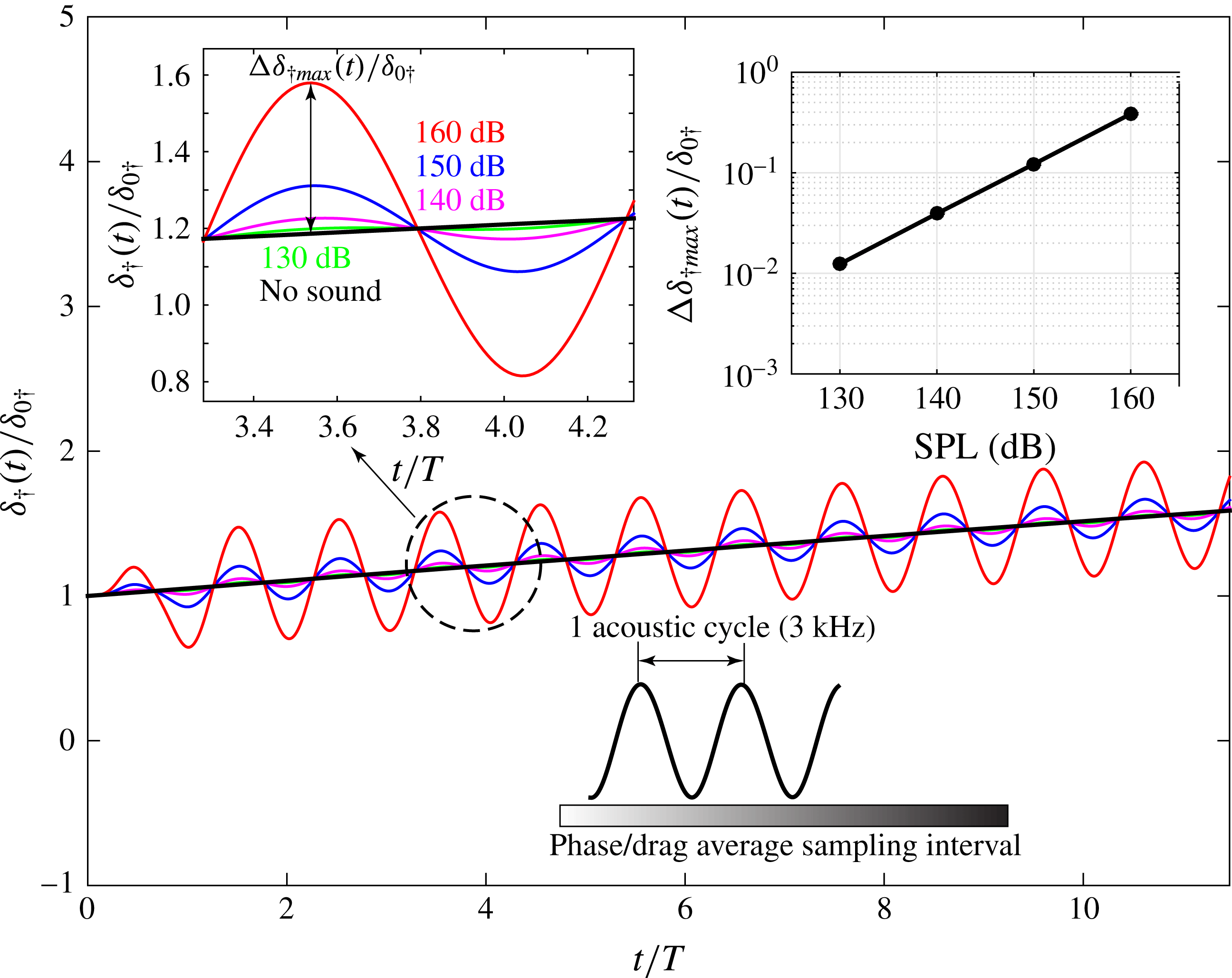
Momentum thickness of the temporally evolving turbulent boundary layer under a normal incident sound at different SPLs.

3 Summary of simulation cases
The simulations proceed by establishing the temporally evolving external flow, either a laminar or turbulent boundary layer, as described in appendix A. The incident plane wave of specified amplitude and frequency impinges upon the facesheet, excites the fluid near the orifice, and is mostly reflected back. Throughout the simulation, the temporally evolving boundary layer slowly thickens, as shown in figure 5, with a modulation due to the incident sound. The phase-averaging presented later was performed over a period of 5 acoustic cycles in which there is a roughly 20 % growth in boundary-layer thickness. We also show that after several initial acoustic cycles, the flow inside the orifice approaches a statistically steady state and the presented quantities do not depend on the boundary-layer growth.
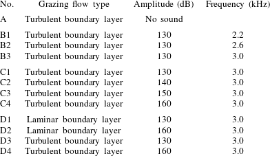
In all, nine different simulations were classified into four sets as shown in table 3. Set (A) contains only one simulation for a turbulent boundary layer grazing the cavity-backed orifice without any incident sound; this case is for reference only. All of the other cases include the incident sound: set (B) contains simulations at variable frequency but fixed 130 dB level that correspond to the GFIT data (M. G. Jones & W. R. Watson 2012, private communication). Set (C) contains the simulations at fixed frequency 3.0 kHz but with variable amplitude from 130 to 160 dB to study the influence of the amplitude of the sound on the flow–orifice interaction. Set (D) contains simulations with fixed frequency 3.0 kHz and either laminar or turbulent boundary layers at both 130 and 160 dB SPL with the goal of investigating the behaviour of the sound-induced flow under different boundary-layer types. Note that some of the cases are repeatedly shown for comparisons.
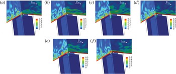
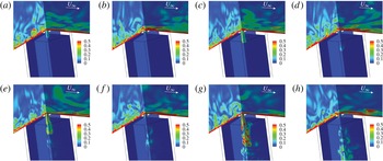
Vorticity contours near the orifice of the liner for set (B) simulations. Slices taken at
 $x=0.0$
,
 $z=0.0$
: (a) 2.2 kHz, inflow; (b) 2.2 kHz, outflow; (c) 2.6 kHz, inflow; (d) 2.6 kHz, outflow; (e) 3.0 kHz, inflow; (f) 3.0 kHz, outflow.

List of the simulations completed in this work.

4 Flow visualization of the sound-induced near-orifice flow
Because of the small orifice sizes used in real world linear applications, visual diagnostics of the near-orifice flow are limited, an exception being the water tunnel visualization studies by Rogers & Hersh (Reference Rogers and Hersh1975). However, semi-empirical modelling can greatly benefit from flow visualization as a means to approximate the complicated fluid mechanics that occurs. This section provides a pictorial representation of the near-orifice flow at the conditions listed in table 3; a quantitative description follows in subsequent sections.
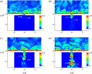
For visualization, vorticity contours taken through the orifice are shown for all the cases from set (B) to set (D) in figure 6 through figure 8, respectively, using the coordinate system in figure 4(b). The presence of the grazing flow clearly breaks the upstream–downstream symmetry of the in-orifice flow so that the flow cannot be considered axisymmetric (cf. Zhang & Bodony Reference Zhang and Bodony2012). The 130 dB sound amplitude case (set B) in figure 6 show minimal penetration of the low-magnitude vorticity into the cavity. The inflow and outflow cycles are qualitatively very different as the exterior grazing flow sweeps downstream the vorticity ejected from the orifice. For this frequency range of 2.2–3.0 kHz very little difference in the flow features are observed.
Vorticity contours near the orifice of the liner under turbulent boundary layer for set (C) simulations. Slices taken at
 $x=0.0$
,
 $z=0.0$
: (a) 130 dB, inflow; (b) 130 dB, outflow; (c) 140 dB, inflow; (d) 140 dB, outflow; (e) 150 dB, inflow; (f) 150 dB, outflow; (g) 160 dB, inflow; (h) 160 dB, outflow.

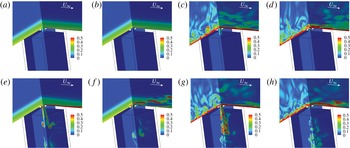
Vorticity contours near the orifice of the liner for set (D) simulations. Slices taken at
 $x=0.0$
,
 $z=0.0$
: (a) 130 dB, laminar, inflow; (b) 130 dB, laminar, outflow; (c) 130 dB, turbulent, inflow; (d) 130 dB, turbulent, outflow; (e) 160 dB, laminar, inflow; (f) 160 dB, laminar, outflow; (g) 160 dB, turbulent, inflow; (h) 160 dB, turbulent, outflow.

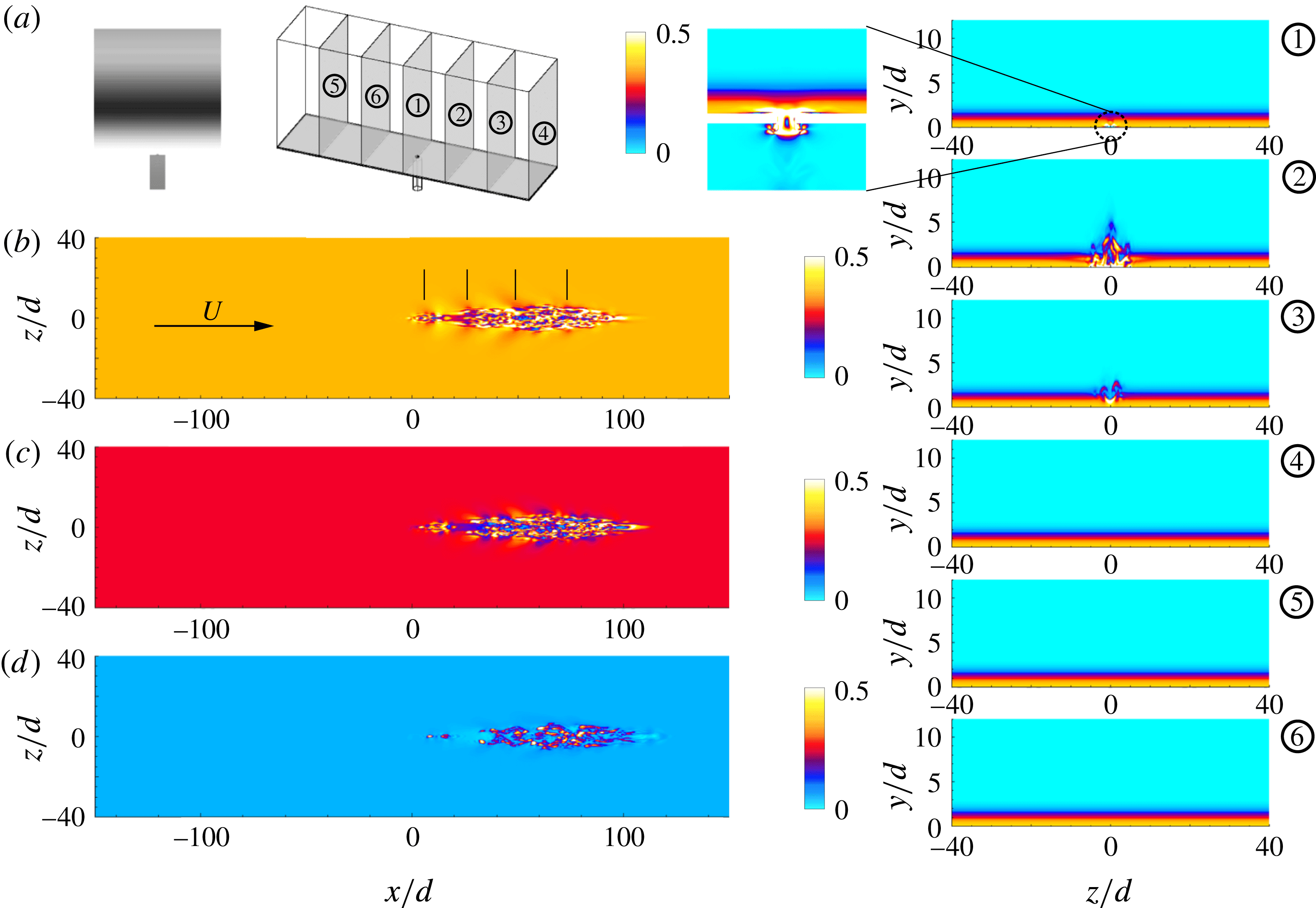
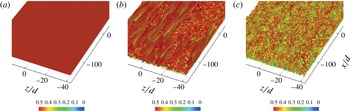
Vorticity magnitude visualization of the cavity-induced transition on an initially laminar boundary layer under 160 dB, 3 kHz, acoustic excitation. The vertical lines in the
 $y=0.5d$
(b) image identify locations excited by constant acoustic phase. (c)
 $y=1.0d$
; (d)
 $2.0d$
.

Figure 7 shows that the penetration depth of the vorticity into the cavity increases with higher sound amplitudes and secondary instabilities develop on the transient jet. The ejection of vorticity, however, shows less visual dependence on the incident sound amplitude with the transient jet being quickly swept downstream and grazing the facesheet.
Whether the grazing boundary layer is laminar or turbulent has a strong influence on the sound-induced flow into the cavity, as shown in figure 8. At 130 dB amplitude the turbulent case is able to more deeply penetrate vorticity into the cavity, presumably when the acoustic and hydrodynamic fields are in phase, while the laminar boundary layer shows very little vorticity generation. For the outflow cycle the ejected vorticity magnitude exceeds that present in the laminar boundary layer but is less than the near-wall vorticity for the turbulent case. At 160 dB the importance of the boundary-layer type is visually apparent in that, for the laminar case, the injected vorticity into the cavity is less intense and more organized into vortex rings as compared to the turbulent boundary-layer case. The ejected vorticity, however, is evidently quite important for the laminar boundary layer at 160 dB as its magnitude exceeds that found in the boundary layer and causes strong boundary-layer disturbances.
At 160 dB the injected vorticity disturbance is sufficiently strong to cause the boundary layer to transition, as shown in figure 9. In the figure, the flow is from left-to-right and contours of streamwise velocity are shown for different heights above the wall and at different downstream planes. The injected vorticity is clearly visible at a distance
 $2d$
above the facesheet and causes significant distortion of the boundary layer as seen in cross-stream plane 2 located approximately
 $70d$
downstream of the orifice. The localized disturbance grows laterally, has a half-angle of approximately nine degrees, and is convected downstream; the boundary layer does not relaminarize. The disturbance is visually consistent with a turbulent spot that is continually fed concentrated vorticity from a fixed location. Because the simulation uses streamwise periodicity the boundary-layer state seen by the orifice changes from laminar towards turbulent; however, the acoustic field is so dominant at 160 dB there is not a statistically significant change in the measured impedance between the laminar and turbulent regimes (see figure 35). At 130 dB, 3 kHz conditions the orifice–sound interaction is much weaker and does not lead to transition, indicating that there is an amplitude threshold, probably weakly dependent on frequency, above which a liner will induce transition. However our parameter space does not allow for us to more precisely quantify this barrier.
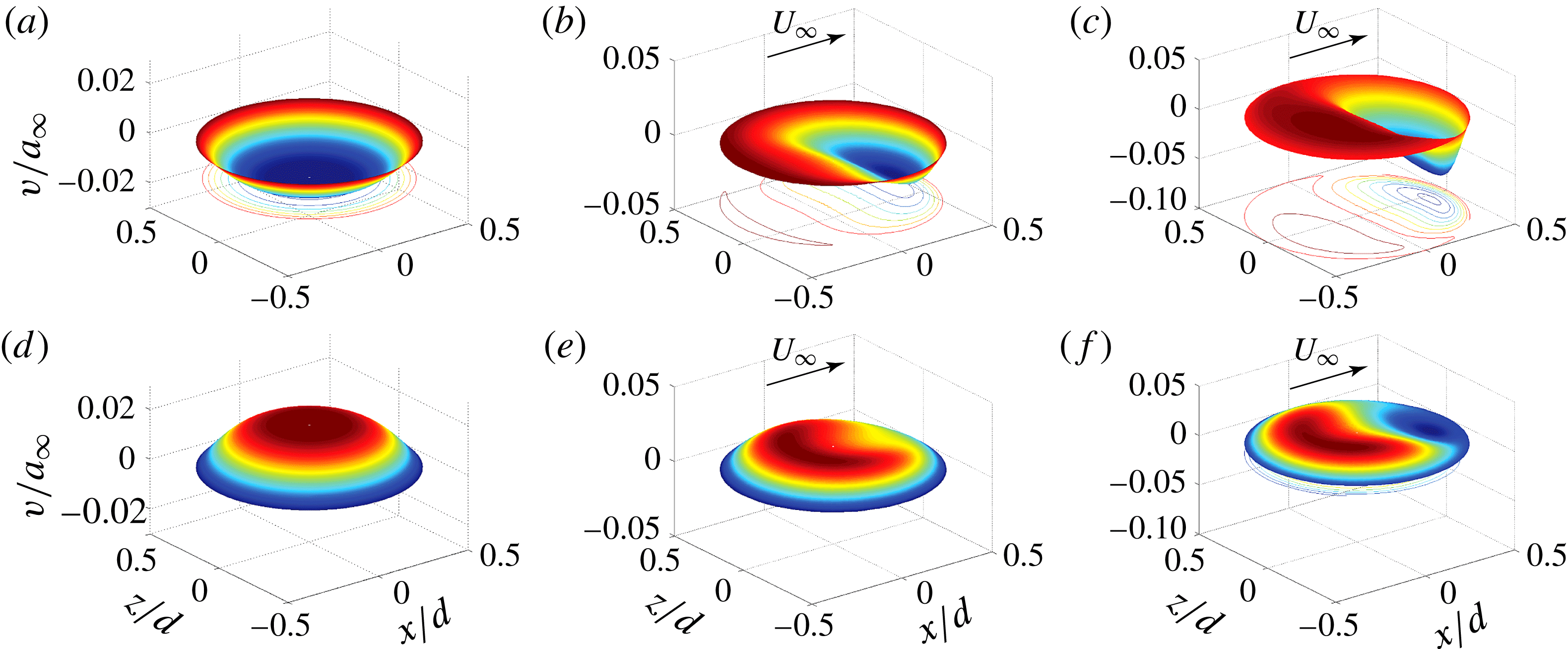
Instantaneous
 $v$
-velocity profile at the mid-plane of the orifice for different grazing flow states and 130 dB, 3 kHz acoustic excitation: (a) no flow, inflow; (b) laminar, inflow; (c) turbulent, inflow; (d) no flow, outflow; (e) laminar, outflow; (f) turbulent, outflow.

5 Velocity profiles near the orifice
The velocity field inside and near the orifice is, from the point of view of the acoustic impedance, the most important consequence of the flow–orifice–sound interaction. In this section we document several different measures of the near-orifice velocity for use in developing a reduced-order impedance model. We first examine the velocity profiles at the centre cut of the orifice.
Schematic of probe locations inside the orifice.

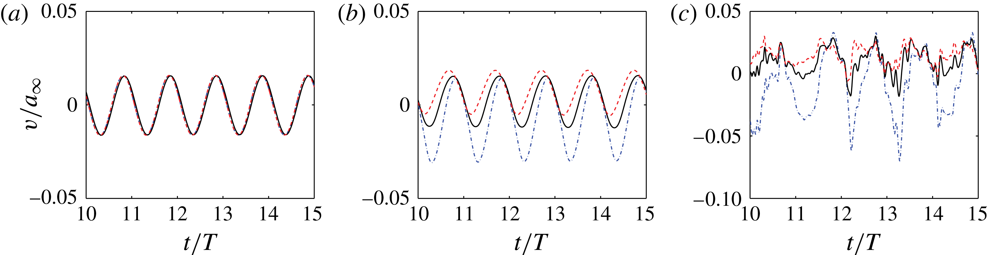
Velocity fluctuations with different grazing flow conditions for simulation B3 (130 dB 3.0 kHz). Legend: - - - -, Probe A; ——, Probe B; — ⋅ —, Probe C: (a) no flow, (b) laminar BL, (c) turbulent BL.

5.1 Mid-facesheet velocity distributions
The impact of the grazing flow on the in-orifice flow can be quickly appreciated by considering the profiles of the orifice-normal velocity taken in the orifice, along the facesheet mid-plane, as shown in figure 10. Conditions without grazing flow and with laminar and turbulent boundary layers are shown for 3 kHz, 130 dB incident sound. The no-flow cases illustrate the azimuthal axisymmetry the velocity profile has when a grazing flow is absent and the profile can be well approximated by hyperbolic tangent curves with a fitted boundary-layer thickness or with periodic pipe flow root-mean-square (r.m.s.) profiles (Zhang & Bodony Reference Zhang and Bodony2012). When a grazing flow is present in the
 $+x$
direction, the azimuthal symmetry is clearly broken and the inflow and outflow cycles are not qualitatively or quantitatively similar, as shown in figure 10(b,c,e,f). Note also that the peak velocity increases by a factor of 2 when the grazing flow is turbulent, and that it is concentrated on the downstream side of the orifice during the inflow cycle. During the outflow cycle the flow is more azimuthally symmetric but still not as much as for the no-flow case.
5.2 Orifice velocity time histories
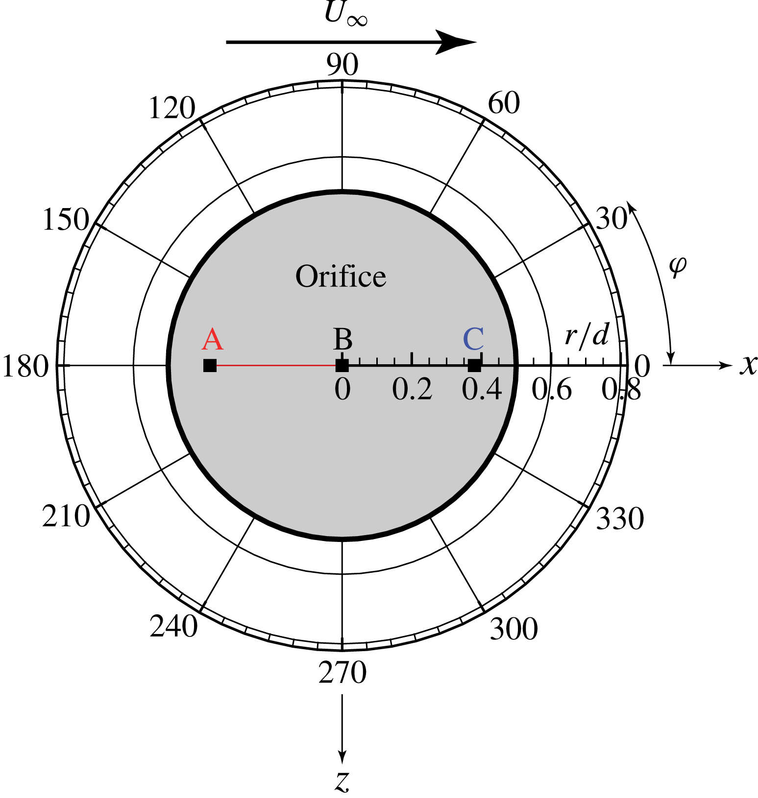
To further quantitatively analyse the biased velocity profiles three probes, labelled A, B and C in figure 11, were placed in the mid-plane of the orifice to record the time history of the velocity fluctuations after the initial transient period. Figure 12 demonstrates the time history of the velocity fluctuations at 130 dB case with different grazing flow conditions. Since the velocity profile has an axisymmetric feature at a quiescent condition, the time history of the velocity fluctuations at A–C collapse. With a laminar boundary layer present, the velocity fluctuations at location A, B and C still remain sinusoidal but with different magnitudes and phases. At Probe A, the velocity fluctuation is nearly always positive, indicating an outflow-dominated motion even during the inflow phase of the incident sound. Although Probe B sits in the centre of the orifice, the velocity fluctuation observed has a positive constant mean value that suggests a biased outflow motion on top of which sits the sound-induced fluctuations. Probe C sits
 $0.36d$
downstream of the origin and reveals a strong motion that is roughly symmetric about
 $v/a_{\infty }=0$
. For the turbulent boundary-layer-induced flow in figure 12(c), the same qualitative picture emerges as in the laminar case but with significant added stochasticity. Again, on average, Probes A and B show an outflow-only and biased outflow, respectively, with roughly the same velocity magnitude peaks, albeit with an increased level of high-frequency (relative to the forcing frequency) fluctuations arising from the boundary layer. Probe C now shows a net inflow character with peak velocities that are roughly 2 times those for the laminar boundary-layer case.
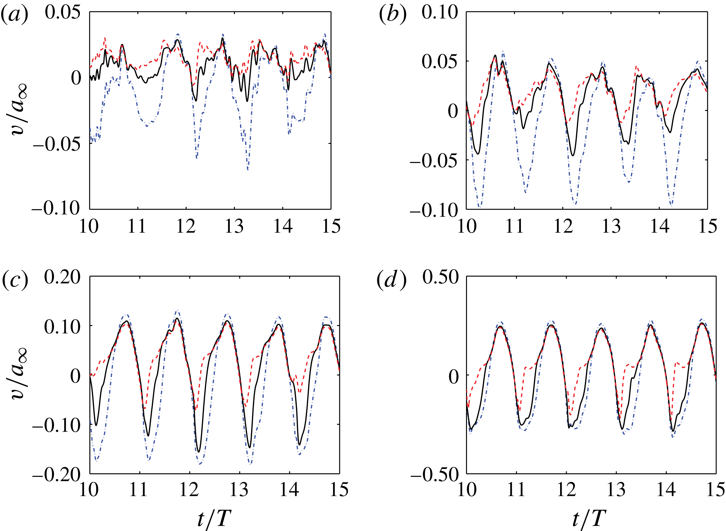
Velocity fluctuations at different SPL with turbulent grazing flow for simulations C1–C4 (3 kHz). Legend: - - - -, Probe A; ——, Probe B; — ⋅ —, Probe C: (a) 130 dB, (b) 140 dB, (c) 150 dB, (d) 160 dB.

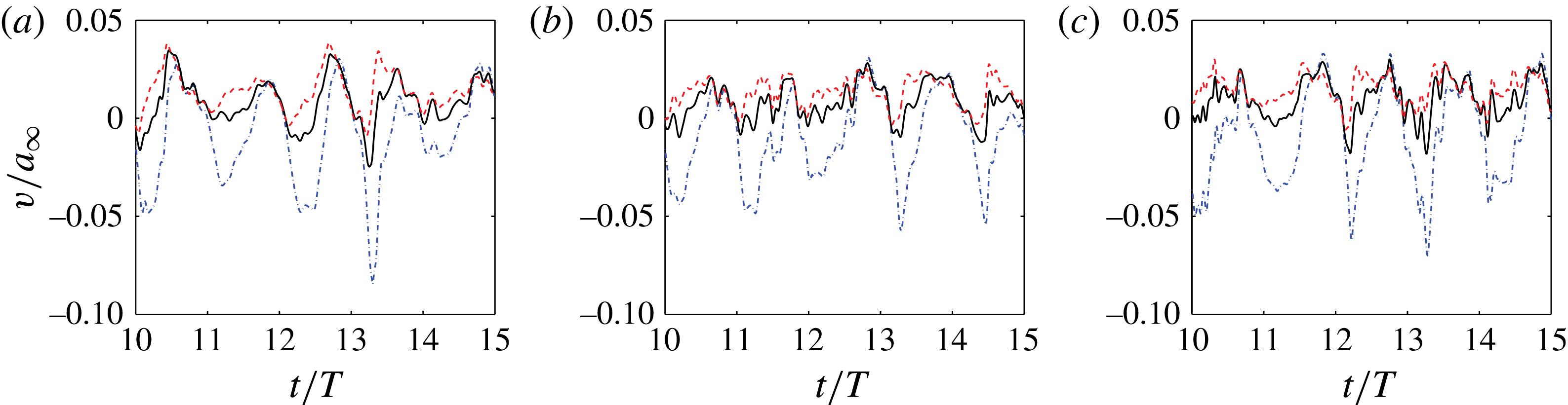
Velocity fluctuations at different frequencies for simulations B1–B3 (130 dB). Legend: - - - -, Probe A; ——, Probe B; — ⋅ —, Probe C: (a) 2.2 kHz, (b) 2.6 kHz, (c) 3.0 kHz.

Figures 13 and 14 demonstrate the effect of changing the sound amplitude or the frequency, respectively, on the velocity history recorded at Probes A, B and C. The velocity fluctuation magnitude increases as the amplitude of the incident sound goes up. The maximum magnitude of the fluctuation reaches roughly 10 %, 18 % and 30 % of the ambient speed of sound for 140 dB, 150 dB and 160 dB, respectively. For reference, a planar acoustic wave would induce velocities of 0.1 %, 0.4 %, 1 % and 4 % of the ambient speed of sound, respectively, indicating the importance of the hydrodynamic field. The additional fluctuations caused by the turbulent boundary layer play a less significant role as the acoustic field becomes stronger and, eventually, the acoustic field overwhelms the hydrodynamic field at 160 dB. Also note that at higher SPLs, the qualitative differences between the fluctuations at different probe locations lessens, indicating a more azimuthally symmetric in-orifice flow. At fixed 130 dB amplitude (see figure 14) the frequency of the incident sound does not appear to influence the in-orifice flow by a large amount.
5.3 Phase-averaged velocity profiles
The in-orifice velocity probes indicated qualitatively different behaviour when a grazing flow was present, with quantitative differences arising from the state of the external boundary layer. They also suggest that in- and outflow cycles arising from the incident sound may be very different. Any future fluid dynamic-based model of the in-orifice flow must take into account these flow asymmetries so, to make the details more accessible for modelling, we construct phase-averaged data conditioned on the incident sound to better describe how the incident sound, orifice wall boundary layers and the grazing boundary layer interact. Our choice is motivated by prior experimental data collected in a water tunnel (Hersh & Rogers Reference Hersh and Rogers1976).
Contour plots of phase-averaged velocity
 $v/a_{\infty }$
with streamlines taken at different phase angles. All cases have a turbulent boundary-layer grazing flow and an incident sound of 3 kHz, cases C1–C4, with amplitude indicated: (a) 130 dB, (b) 140 dB, (c) 150 dB, (d) 160 dB.

Contour plots of phase-averaged velocity
 $v/a_{\infty }$
with streamlines taken at different phase angles. All cases have an incident sound of frequency 3 kHz with amplitude and boundary-layer state indicated, cases D1–D4: (a) 130 dB laminar BL, (b) 130 dB turbulent BL, (c) 160 dB laminar BL, (d) 160 dB turbulent BL.

Referring to figure 11, phase-averaged data are extracted along a plane with normal in the transverse direction
 $+z$
, corresponding to
 ${\it\varphi}=0^{\circ },\,180^{\circ }$
. The plane cuts through the middle of the orifice,
 $x=0$
. The phase angle
 ${\it\phi}$
of the incident sound is taken relative to the sound as it impacts the plate with
 ${\it\phi}=0$
being the beginning of the inflow cycle and
 ${\it\phi}={\rm\pi}$
being the beginning of the outflow cycle.
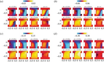
The images in figure 15 show how the phase-averaged flow varies with
 ${\it\phi}$
and between cases of different amplitude at a 3 kHz constant frequency, cases C1–C4. Only the region in the orifice’s immediate vicinity is shown with a small portion of the facesheet visible. Considering first the 130 dB incident case in figure 15(a) it is clear that during the inflow cycle the near-orifice flow shares resemblance to a driven cavity flow wherein, for sufficiently low Reynolds number, a vortex sits in the upstream side and drives a circulatory flow within the orifice. The analogy is imprecise in that the strength of the induced flow depends both on the grazing boundary-layer-applied shear and the incident pressure field, as noted in the other phase angles between
 ${\it\phi}={\rm\pi}/4$
and
 ${\it\phi}={\rm\pi}$
. During the outflow cycle, where
 ${\rm\pi}\leqslant {\it\phi}\leqslant 2{\rm\pi}$
, the upstream vortex disappears and the driven cavity analogy fails. Instead, the in-orifice flow more resembles that expected from our earlier work without a grazing flow present; it is only when the ejected flow passes the plane of the facesheet that the grazing flow appears to be effective. At higher acoustic sound amplitudes the influence of the upstream vortex reduces and the analogy further degrades. It is always true that, during the inflow cycle, the fluid that is able to get into the cavity enters from the downstream side while, during the outflow cycle, the downstream bias is nearly absent. The origin of this asymmetry is, of course, the asymmetry in the flow exterior to the orifice – either the on the facesheet side or within the cavity – but its presence is crucial to effectively modelling the flow. More quantitative measures of the asymmetry will be given later in §§ 5.5.2 and 5.6.
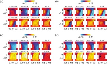
Figure 16 again looks at the phase-averaged view of the near-orifice flow but focuses on the influence of the state of the external boundary layer for the 130 and 160 dB incident sound cases, all at 3 kHz. During the inflow cycle for 130 dB sound the laminar and turbulent boundary-layer state has a strong influence on the size and effective strength of the upstream vortex, in analogy to the driven cavity, where the stronger mean shear from the turbulent boundary layer creates a stronger induced flow within the orifice. At 160 dB incident the inflow cycle depends only weakly on the boundary-layer state, an observation that carries over to the outflow cycles at both sound amplitudes.
5.4 Dimensionless parameters
In the foregoing analysis it was shown that the in-orifice flow is influenced by the combined effects of the incident acoustic field and the grazing flow. We now examine how to scale the data.
5.4.1 Velocity scale
There are several candidate velocity scales from which to choose, including the grazing flow velocity,
 $U_{\infty }$
, the velocity associated with the incident sound field,
 $|p^{\prime }|/({\it\rho}_{\infty }a_{\infty })$
and the sound-induced velocity in a Helmholtz resonator. In addition one may consider velocity scales associated with the turbulent boundary layer. We focus on the linear response of the lumped element of the Helmholtz resonator without a grazing flow, which yields (Morse & Ingard Reference Morse and Ingard1968)
 $$\begin{eqnarray}\displaystyle v_{ac}^{\prime }=\frac{|p^{\prime }|}{{\it\rho}{\it\omega}({\it\tau}+0.8d)}\frac{1}{\displaystyle \sqrt{\left[\left(\frac{{\it\omega}_{H}}{{\it\omega}}\right)^{2}-1\right]+\left(\frac{{\it\omega}_{H}}{{\it\omega}Q}\right)^{2}}}, & & \displaystyle\end{eqnarray}$$
where
 ${\it\omega}_{H}$
was given in (1.1) and
 $Q$
is the quality factor with a typical factor of 10. Note that in the high-frequency limit (
 ${\it\omega}/{\it\omega}_{H}\gg 1$
) we consider, the approximation can be made
 $$\begin{eqnarray}\displaystyle v_{ac}^{\prime }\approx \frac{|p^{\prime }|}{{\it\rho}{\it\omega}({\it\tau}+0.8d)}. & & \displaystyle\end{eqnarray}$$
This method generally provides a very good magnitude estimate for the sound induced in-orifice flow in quiescent conditions but has not been evaluated when a grazing flow is present.
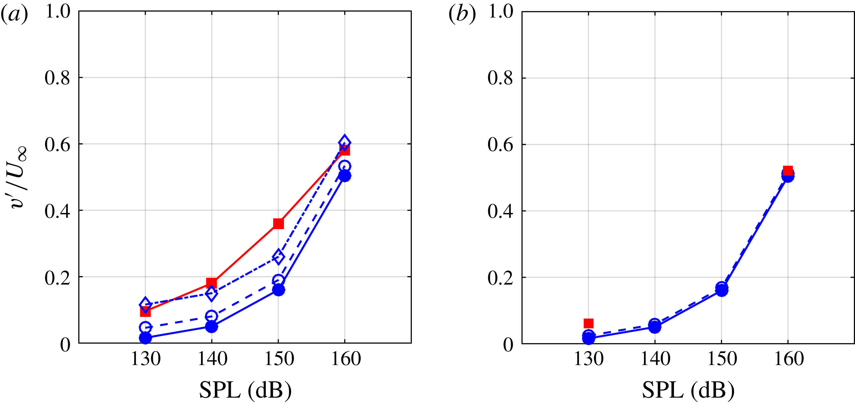
The simulation databases were processed to extract the average maximum in-orifice velocity for the cases listed in table 3. These values are to be denoted by
 $v_{peak}^{\prime }$
and are plotted in figure 17 and compared to the
 $v_{ac}^{\prime }$
values from (5.2) for 3 kHz incident acoustic fields and a turbulent boundary-layer grazing flow. For the turbulent boundary cases there is good qualitative agreement between the two velocity scales as the SPL increases but they differ by a near-constant value of approximately
 $0.1U_{\infty }$
; namely,
 $v_{peak}^{\prime }\approx 0.1U_{\infty }+v_{ac}^{\prime }$
. It is clear that at the highest sound amplitude case the importance of the boundary layer is reduced so that
 $v_{peak}^{\prime }\approx v_{ac}^{\prime }$
. For the laminar boundary-layer cases, shown in figure 17(b), there is closer agreement between the two velocity scales but again an offset appears. Whether
 $v_{peak}^{\prime }$
or
 $v_{ac}^{\prime }$
better scales the data will be discussed next along with a means to estimate
 $v_{peak}^{\prime }$
from
 $v_{ac}^{\prime }$
.
Comparison between the theoretical peak orifice velocity and the DNS data at different SPLs at 3 kHz. Legend: –▪–, DNS peak velocity
 $v_{peak}^{\prime }$
; –●–, theoretical acoustic velocity
 $v_{ac}^{\prime }$
given by (5.2); –○–, estimate
 $\tilde{v}_{peak}^{\prime }$
using
 ${\it\alpha}=0$
and
 ${\it\beta}=0.6$
; –♢–, estimate
 $\tilde{v}_{peak}^{\prime }$
using
 ${\it\alpha}=1$
and
 ${\it\beta}=0.6$
: (a) turbulent BL, (b) laminar BL.

5.4.2 Strouhal and Reynolds number
With the proper quantification of the in-orifice velocity shown above, we can determine the Strouhal and Reynolds numbers based upon the orifice flow conditions,
 $$\begin{eqnarray}\displaystyle Sr=\frac{{\it\omega}d}{v_{o}^{\prime }}\quad Re_{d}=\frac{v_{o}^{\prime }d}{{\it\nu}}, & & \displaystyle\end{eqnarray}$$
where
 $v_{o}^{\prime }$
is the in-orifice flow velocity. A simple computation of
 $Sr$
and
 $Re_{d}$
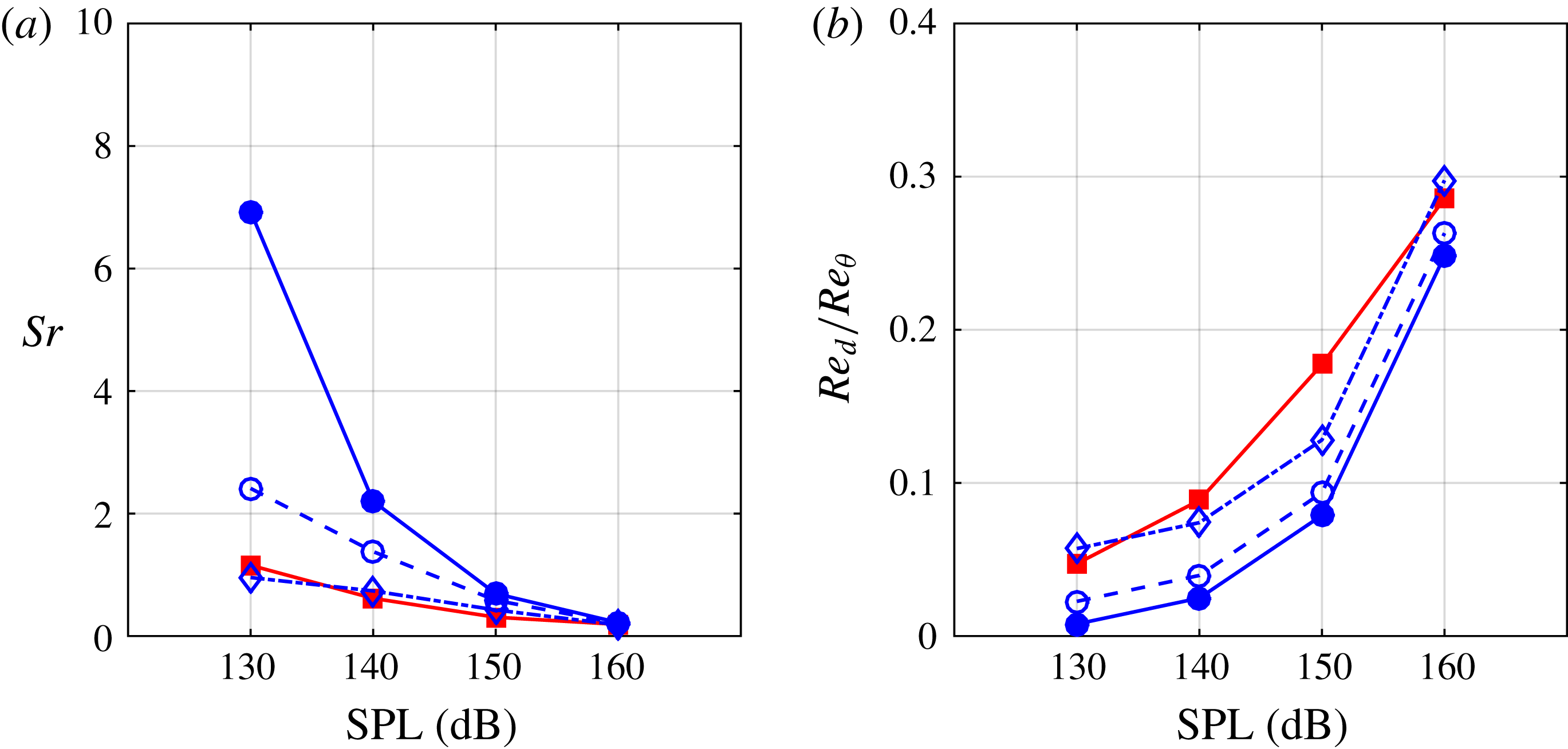
using the two velocity scales is given in figure 18.
Importantly, the inverse Strouhal number
 $1/Sr$
indicates how far into the cavity the sound-induced fluid can penetrate. Using the DNS databases we evaluate the predictive measure of
 $1/Sr$
using the two velocity scales, as marked by arrows, in figure 19. Both velocity scales are reasonable but the DNS-measured scale of
 $v_{peak}^{\prime }$
yields a better estimate of the fluid penetration depth over 130–160 dB incident sound amplitude range.
Strouhal number and Reynolds number (scaled by the boundary layer Reynolds number) for the in-orifice flow at different SPLs, 3 kHz, and turbulent grazing boundary layer. Legend: see figure 17: (a) Strouhal number, (b) Reynolds number.

Vorticity magnitude at inflow peak phase (
 ${\it\phi}=1/2{\rm\pi}$
). Marks: right arrow (
 $\rightarrow$
) indicates the location of
 $1/Sr^{(ac)}$
; left arrow (
 $\leftarrow$
) indicates the location of
 $1/Sr^{(p)}$
.

5.4.3 Estimating
 $v_{peak}^{\prime }$

The data of figures 17–19 demonstrate that the small difference between
 $v_{ac}^{\prime }$
and
 $v_{peak}^{\prime }$
is important. To estimate the difference we recall the flow visualizations of § 5 and the observation that both the presence of a grazing flow and the state of that grazing flow were important. We hypothesize that these two physical can be used to derive scaling results that more closely connect
 $v_{ac}^{\prime }$
and
 $v_{peak}^{\prime }$
.
Referring to figures 6–8 we observe that when the boundary layer is turbulent there is an additional penetration of fluid into the orifice, indicating that the boundary-layer disturbances contribute to the sound-induced flow. A crude estimate of this effect is to assume that the horizontal velocity fluctuations within the boundary layer are transported into the orifice through the sound-associated pressure gradient. This implies that an additional velocity fluctuation of the order of
 $u_{rms}^{\prime }$
should be added to
 $v_{ac}^{\prime }$
.
The phase-averaged data shown in figures 15 and 16 have a flow pattern analogy to a lid-driven cavity (Botella & Peyret Reference Botella and Peyret1998). Even though the analogy is imperfect it suggests that the shear-driven flow near the facesheet side of the orifice contributes to the in-orifice velocity. Thus the wall friction velocity
 $u_{{\it\tau}}=\sqrt{{\it\tau}_{w}/{\it\rho}}$
is the appropriate velocity scale.
Combining these two additional velocity scales yields an estimate of
 $$\begin{eqnarray}\displaystyle \tilde{v}_{peak}^{\prime }=v_{ac}^{\prime }+{\it\alpha}u_{rms}^{\prime }+{\it\beta}u_{{\it\tau}}, & & \displaystyle\end{eqnarray}$$
where
 ${\it\alpha}$
and
 ${\it\beta}$
are constants that are of order one. The driven cavity literature has established that
 ${\it\beta}\approx 0.6$
, assuming
 $u_{{\it\tau}}$
is the effective lid velocity, for a range of Reynolds numbers while
 ${\it\alpha}\approx 1$
is justified based on the flow visualizations and additional data shown in figure 14.
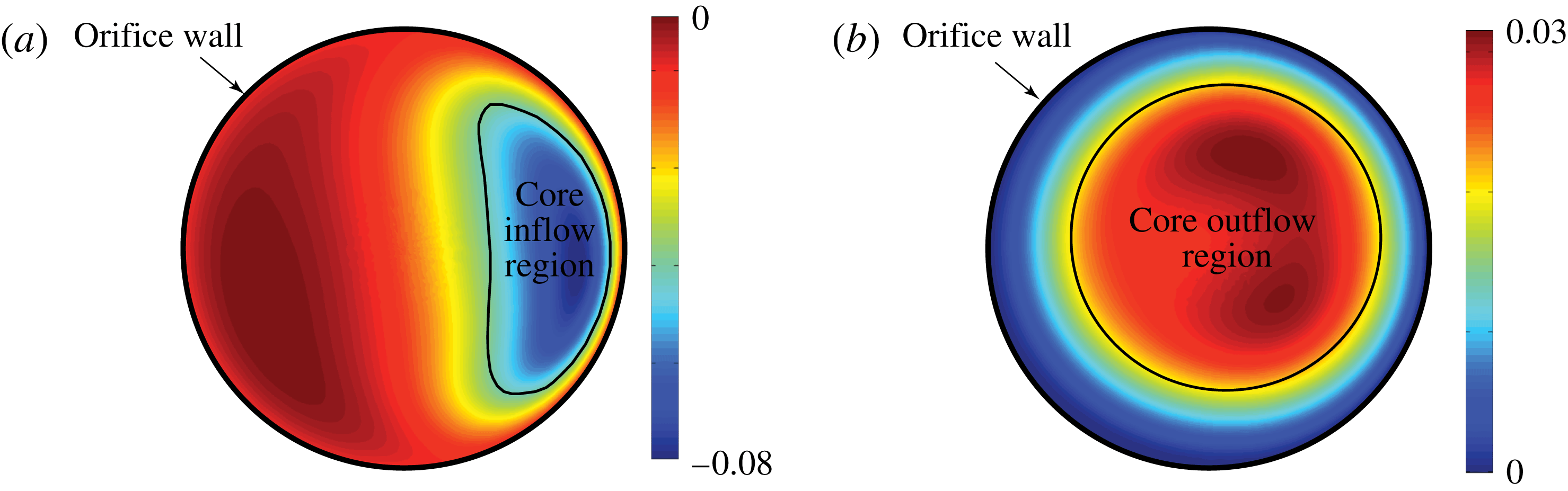
Schematic of the definition for core flow region. Contours of vertical velocity
 $v/a_{\infty }$
are shown with identified inflow and outflow regions: (a) inflow cycle, (b) outflow cycle.

Figures 17–19 clearly show that the estimate
 $$\begin{eqnarray}\displaystyle \tilde{v}_{peak}^{\prime }=v_{ac}^{\prime }+u_{rms}^{\prime }+0.6u_{{\it\tau}} & & \displaystyle\end{eqnarray}$$
yields a reasonable prediction of
 $v_{peak}^{\prime }$
measured from the DNS data, as well as through the corresponding Strouhal and Reynolds numbers. Observe that a useful velocity scale required information on both the grazing flow and its state for quantitative accuracy.
5.5 Discharge coefficient
5.5.1 Instantaneous discharge coefficient
The rate of fluid that reaches into the cavity, which is closely related to the discharge coefficient, strongly determines the acoustic behaviour of the liner. Previous work without a grazing flow (Zhang & Bodony Reference Zhang and Bodony2012) showed that a useful way to approximate the discharge coefficient was to consider the boundary-layer growth along the inner orifice walls; however, in that case the flow was axisymmetric. With the presence of the grazing flow, difficulties immediately arise as the flow pattern is no longer axisymmetric and theoretical results for boundary layers in this environment are not useful. Therefore, we must use a different way to predict the discharge coefficient – one that does not directly rely upon orifice boundary layers – when a grazing flow is present. Figure 20 demonstrates the basic idea of our estimation of the discharge coefficient prediction that relies on the ratio between the core inflow-to-outflow area, as identified by the sign of
 $v$
,
 $$\begin{eqnarray}\displaystyle C_{Di}=\frac{4A_{i}}{{\rm\pi}d^{2}}\quad C_{Do}=\frac{4A_{o}}{{\rm\pi}d^{2}}, & & \displaystyle\end{eqnarray}$$
where
 $A_{i}$
and
 $A_{o}$
are the inflow and outflow areas, respectively. In essence, we are tracking the percentage area of the orifice that flow enters or departs from the cavity, as expected from the acoustic field since, as figure 20 shows, there is usually flow simultaneously entering and leaving the orifice. The task to predict the discharge coefficient now requires an evaluation of the core flow area which is, unfortunately, one step removed from a more basic physical phenomena of a boundary layer.
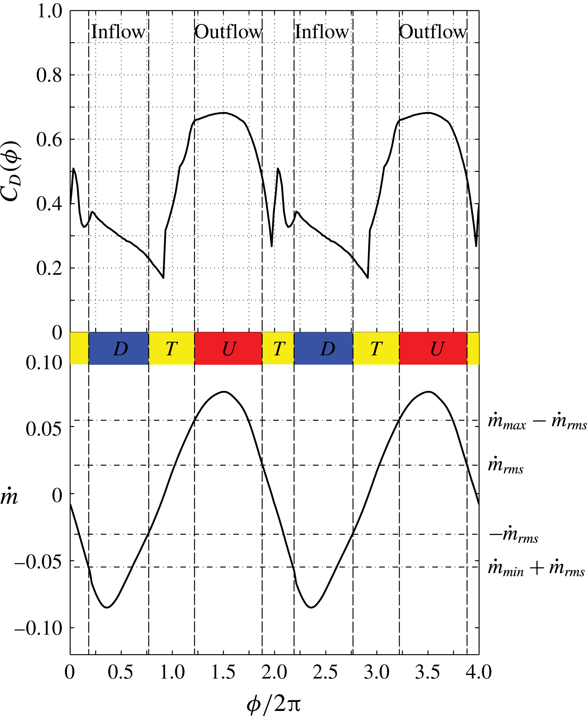
Because of the flow reversal it is challenging to assign a single value for the core flow area. Further, the qualitatively different behaviour for the inflow and outflow cycles requires us to differentiate the discharge coefficient between them. Therefore, we split the whole acoustic cycle into four different periods, following earlier work (Zhang & Bodony Reference Zhang and Bodony2012). In figure 21, the labels ‘D’ and ‘U’ represent downward and upward motion respectively while label ‘T’ represents transition period. Identification of these periods is derived from the mass flow rate, as follows: the phase-averaged mass flow rate,
 ${\dot{m}}({\it\phi})$
, is computed for each simulation and its r.m.s., minimum and maximum values are recorded. The inflow cycle is defined when by those angles
 ${\it\phi}$
such that
 ${\dot{m}}({\it\phi})\leqslant {\dot{m}}_{min}+{\dot{m}}_{rms}$
and, likewise, the outflow cycle is defined by
 ${\dot{m}}({\it\phi})\geqslant {\dot{m}}_{max}-{\dot{m}}_{rms}$
. Those angles
 ${\it\phi}$
outside of these two ranges are the transition periods. An example analysis of this type is shown in figure 21 for the 160 dB, 3 kHz, interaction where the inflow and outflow cycles are very different with
 $C_{D}$
values between 0.2 and 0.4 during the inflow and between 0.5 and 0.67 for the outflow cycle, with the latter showing a nearly constant value around 0.65 for most of the outflow cycle. Recall that
 $C_{D}\approx 1$
implies very little blockage of the flow entering or exiting the orifice and that
 $C_{D}\approx 0.76$
is the industry standard for single degree-of-freedom Helmholtz resonator liners (Motsinger & Kraft Reference Motsinger, Kraft and Hubbard1995). The
 $C_{D}({\it\phi})$
behaviour for the other incident sound cases are qualitatively similar but quantitatively different and not shown here; instead they may be found in Zhang (Reference Zhang2014).
Instantaneous discharge coefficient for liner with 160 dB, 3 kHz incident sound and a turbulent boundary-layer grazing flow.

5.5.2 Averaged discharge coefficient
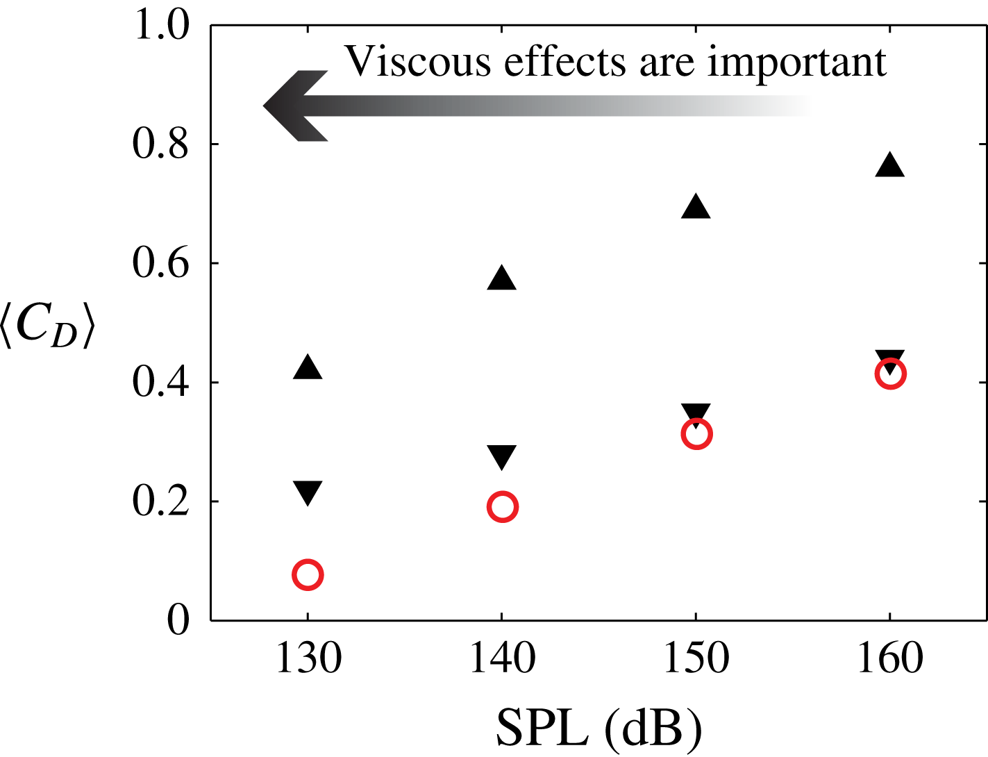
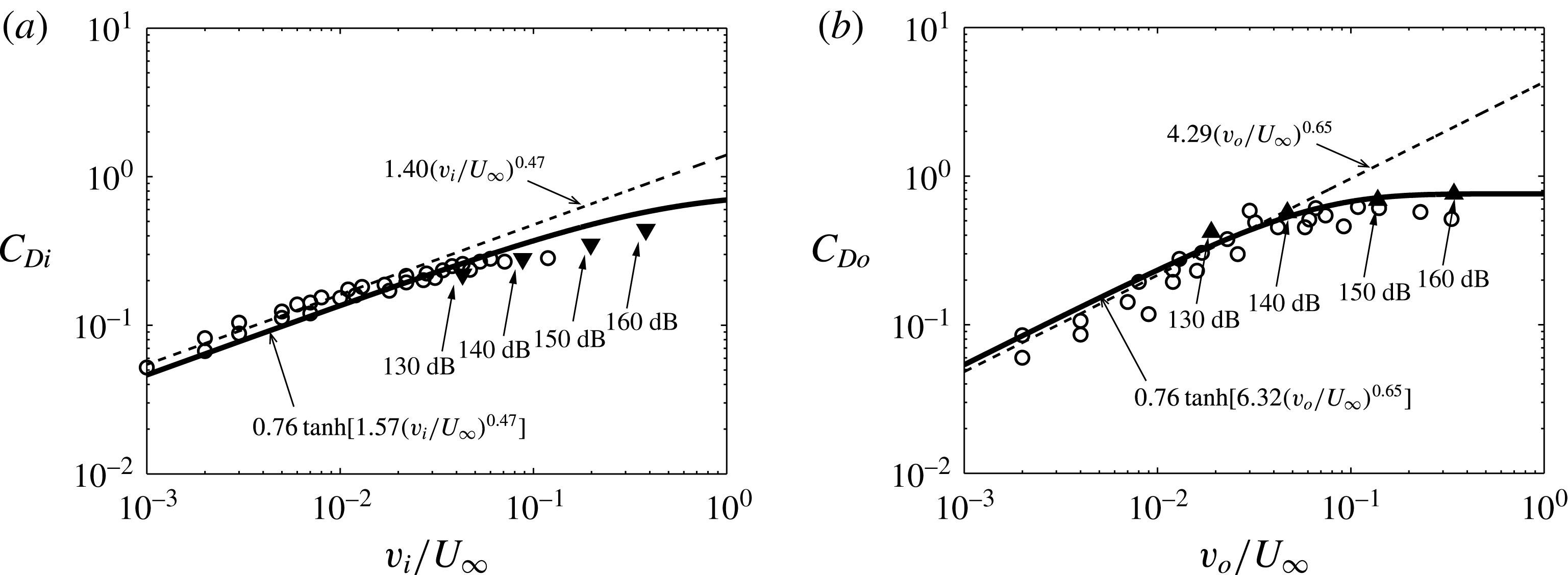
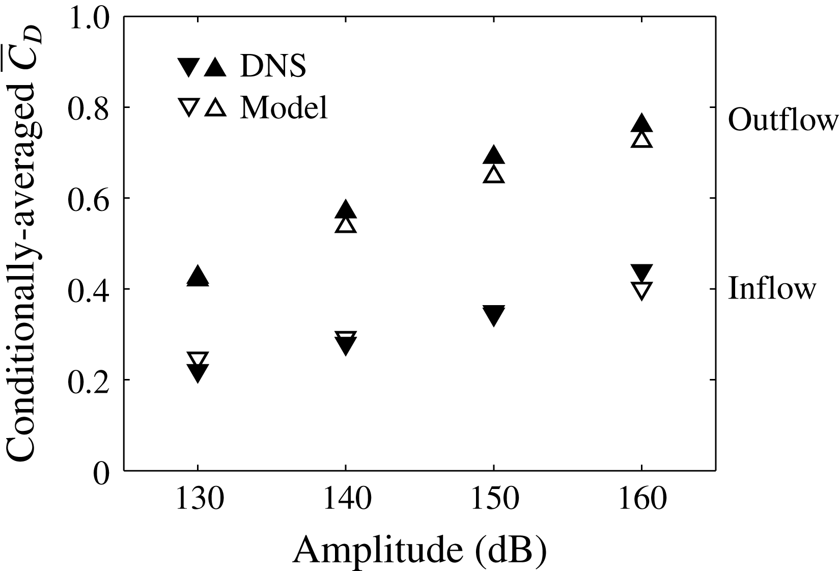
By conditionally averaging the instantaneous discharge coefficient at the inflow and outflow periods, we obtain the averaged inflow and outflow discharge coefficient shown in figure 22. Note that the inflow discharge coefficient is always lower than the outflow discharge coefficient at the same SPL, caused by the separation of the flow from the upstream side of the orifice, as shown in figures 15 and 16. For the inflow cycle, the averaged discharge coefficient matches the empirical prediction from Tonon et al. (Reference Tonon, Moers and Hirschberg2013) at high SPL (150, 160 dB). The predictions for the cases with lower SPLs (130 and 140 dB), however, deviate from the empirical inflow discharge coefficient model as the viscous effects become more important. Also note that the discharge coefficients show a linear increase with the increase of the amplitude of the sound except at 160 dB outflow period, where the discharge coefficient reaches nearly 0.76.
Phase-averaged discharge coefficient at different SPLs under a turbulent boundary layer, all at 3.0 kHz. Legend: ▴, outflow discharge coefficient; ▾, inflow discharge coefficient; ○, empirical model prediction of inflow discharge coefficient from Tonon et al. (Reference Tonon, Moers and Hirschberg2013).

We can further average the inflow and outflow discharge coefficients to obtain a globally averaged discharge coefficient
 $\overline{C}_{D}$
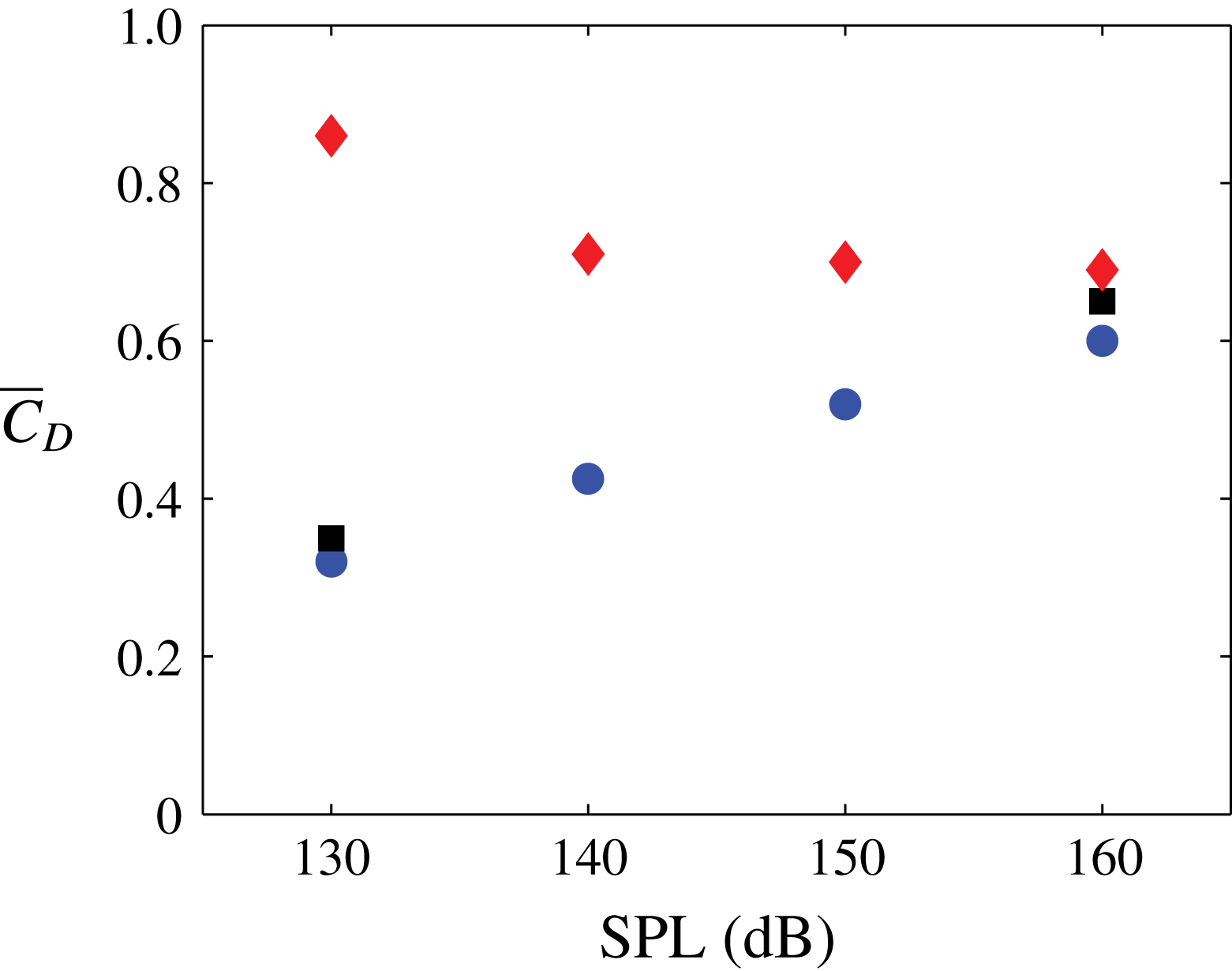
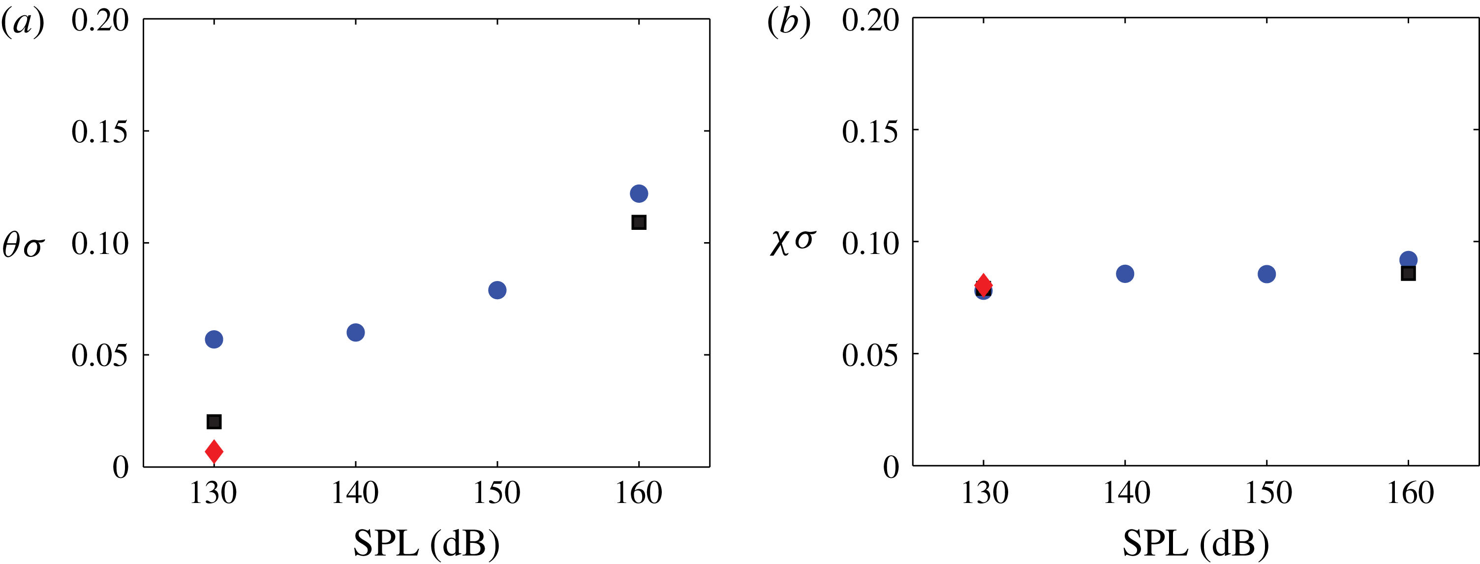
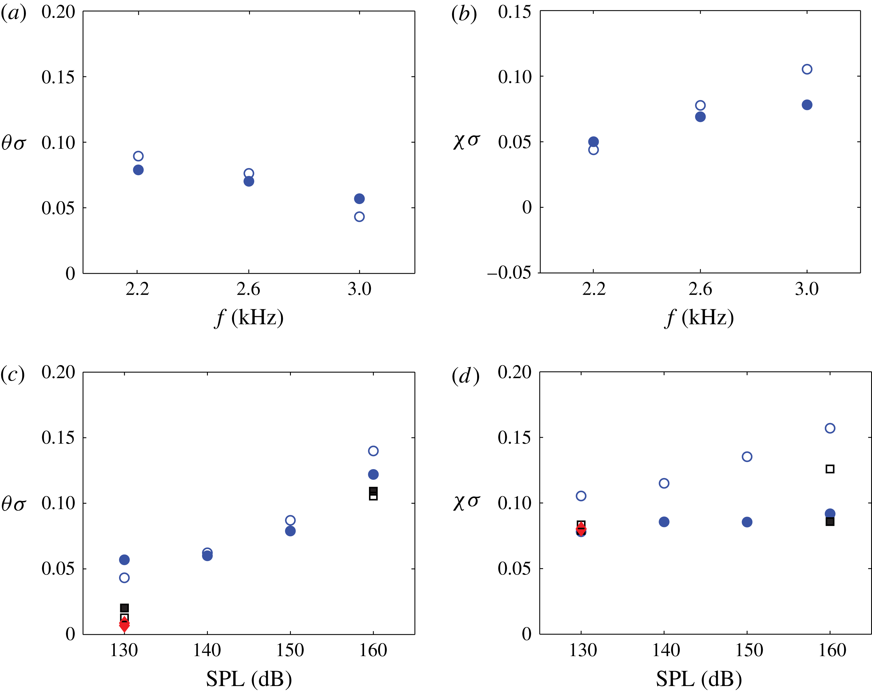
for the whole acoustic cycle. This parameter is especially useful for reduced-order modelling and will be discussed later. Comparisons of the global discharge coefficient between the no grazing flow, laminar boundary layer and turbulent boundary-layer cases are shown in figure 23.
Comparison of the globally averaged discharge coefficient under different grazing flow conditions and 3 kHz acoustic excitation. Legend: ♦, no grazing flow; ▪, laminar boundary layer; ●, turbulent boundary layer.

At fixed SPL, the grazing flow condition acts to lower the discharge coefficient value by ‘blocking’ the fluid from going into and out of the orifice. The influence of the grazing flow diminishes with increasing SPL so that the difference between the no-flow, laminar, and turbulent flow values of
 $\overline{C}_{D}$
also diminishes. Also note that the discharge coefficient is slightly higher for the cases with laminar boundary layer than the ones with the turbulent boundary layer. Another interesting observation is that the trend of the global discharge coefficient behaves oppositely whether there is a grazing flow: with grazing flow the discharge coefficient increases as the SPLs increases while a decreasing trend is observed for the cases at quiescent condition.
The reason for the different trends is relatively straightforward, given the flow visualization in figures 15 and 16, and prior results in Zhang & Bodony (Reference Zhang and Bodony2012). In the absence of a grazing flow, the orifice boundary layers directly control the discharge coefficient: at low acoustic amplitudes and at frequencies away from resonance the orifice boundary layers are laminar, quasi-steady and thin. As the sound amplitude increases, orifice-generated vorticity interacts with the boundary layers, thickens them, eventually causing them to separate, leading to a smaller discharge coefficient. When a grazing flow is present, the orifice boundary layers are not dynamically important because of the near-wall inertia-induced separation from the upstream orifice that effectively constricts the useful area in which sound can induce flow within the orifice. As the sound amplitude increases, this constriction is less dynamically effective as the acoustic field is so strong, and the orifice dynamics approaches that when the grazing flow is not present.
It is important to note that these observations are qualitatively consistent with the data but the rates of change of
 $C_{D}$
with sound amplitude, frequency and grazing flow Mach number must depend directly on these parameters since, for example, a stronger grazing flow would likely require a stronger acoustic field before approaching the quiescent values of
 $C_{D}$
.
5.6 Pressure statistics
In estimating the discharge coefficient in § 5.5, it was observed that the qualitative time histories of point measurements taken within the orifice changed dramatically with sound amplitude. To quantify this observation, time traces of the pressure were taken within the orifice and their autocorrelations,
 $\mathscr{R}(t)$
, were used to compute the integral time scale according to
 $$\begin{eqnarray}\displaystyle \mathscr{T}=\int _{0}^{\infty }\mathscr{R}(t)\,\text{d}t. & & \displaystyle\end{eqnarray}$$
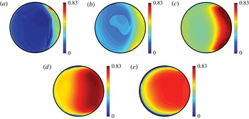
Because the data are not phase averaged, the integral time scale indicates whether the probe sees a pressure field that is dominated by the turbulent hydrodynamic field (with a relatively short time scale) or the incident acoustic field (with a relatively long time scale) and could be used as an alternative measure for estimating the discharge coefficient. The data are shown in figure 24, normalized by the acoustic period, where the impact of the sound field is clear: as the sound amplitude increases, its influence over the in-orifice dynamics increases and imposes its time scale upon the flow until, eventually, the impact of the turbulent boundary layer on the in-orifice flow is confined to a decreasingly small region near the upstream orifice wall. Similar results hold for the vertical velocity component but are not shown for space.
Contour plot of the integral time scale of the pressure, relative to the acoustic period, over the orifice for the case of 3.0 kHz incident sound with a turbulent boundary layer at the indicated sound amplitudes: (a) no sound, (b) 130 dB, (c) 140 dB, (d) 150 dB, (e) 160 dB.

6 Drag analysis
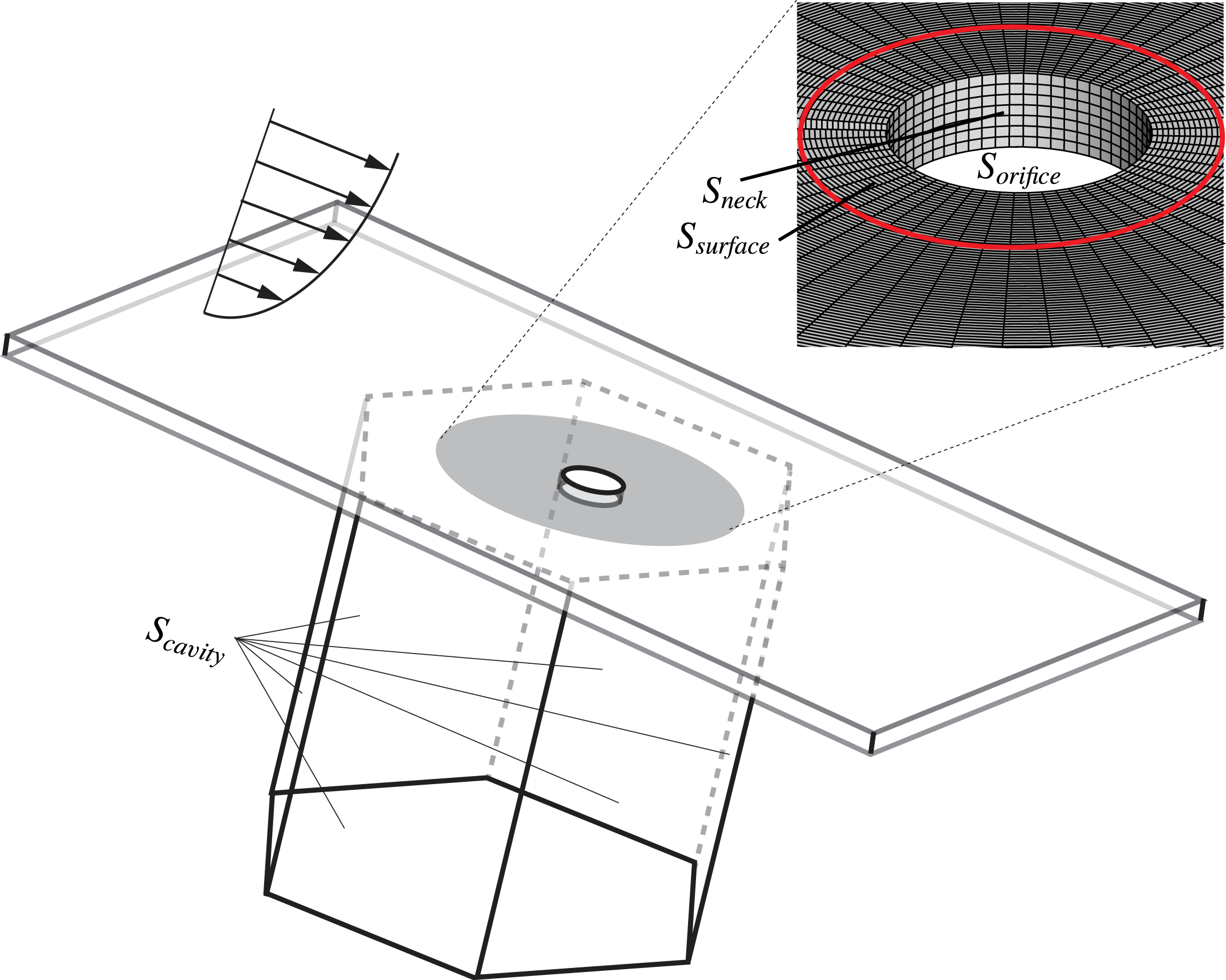
Introducing an acoustic liner can affect the overall drag experienced by an aircraft; however, precise measurements of whether liners increase or decrease drag are rare. The recent paper by Tam et al. (Reference Tam, Pastouchenko, Jones and Watson2014) estimated the drag change due to their slit liner by counting the rotational kinetic energy bound to vortices shed per unit time; that method is not useful for turbulent flows with distributed vorticity. More recently experimental methods are being developed to estimate liner drag from in situ flow measurements (Howerton & Jones Reference Howerton and Jones2015; Gerhold, Brown & Jasinski Reference Gerhold, Brown and Jasinski2016); both studies indicate liners cause increased drag. Instead we can directly measure the surface stresses present and integrate them over the liner. Our integration domain is shown in figure 25 where the facesheet surface (
 $S_{surface}$
), cavity (
 $S_{cavity}$
) and orifice walls (
 $S_{neck}$
) are identified. Furthermore, the open area exposed by the orifice, denoted by
 $S_{orifice}$
, is used to compare drag measurements for cases without an orifice. In Zhang (Reference Zhang2014) it was shown that the viscous stresses are important only on the facesheet and not on the orifice. With these definitions, for the case when the orifice and cavity are absent the overall force is
 $$\begin{eqnarray}\displaystyle \boldsymbol{F}_{no}=\int _{S_{surface}+S_{orifice}}\boldsymbol{f}\,\text{d}S, & & \displaystyle\end{eqnarray}$$
where
 $\boldsymbol{f}=-p\hat{\boldsymbol{n}}+{\bf\tau}\hat{\boldsymbol{n}}$
is the surface traction for a surface with unit outward normal
 $\hat{\boldsymbol{n}}$
, pressure
 $p$
and viscous stress tensor
 ${\bf\tau}$
. When a cavity is present, the expression integrated is
 $$\begin{eqnarray}\displaystyle \boldsymbol{F}_{wo}=\int _{S_{surface}}\boldsymbol{f}\,\text{d}S-\int _{S_{neck}+S_{cavity}}p\hat{\boldsymbol{n}}\,\text{d}S. & & \displaystyle\end{eqnarray}$$
For convenience we take
 $S_{surface}=11.5S_{orifice}$
(the non-open-area for an 8.7 % porosity liner) so that we do not perform the facesheet integration over the entire domain and rely on the difference of two large numbers to measure the drag. It has been confirmed in Zhang (Reference Zhang2014) that drag change conclusions are not sensitive to this choice.
Schematic of drag evaluation.

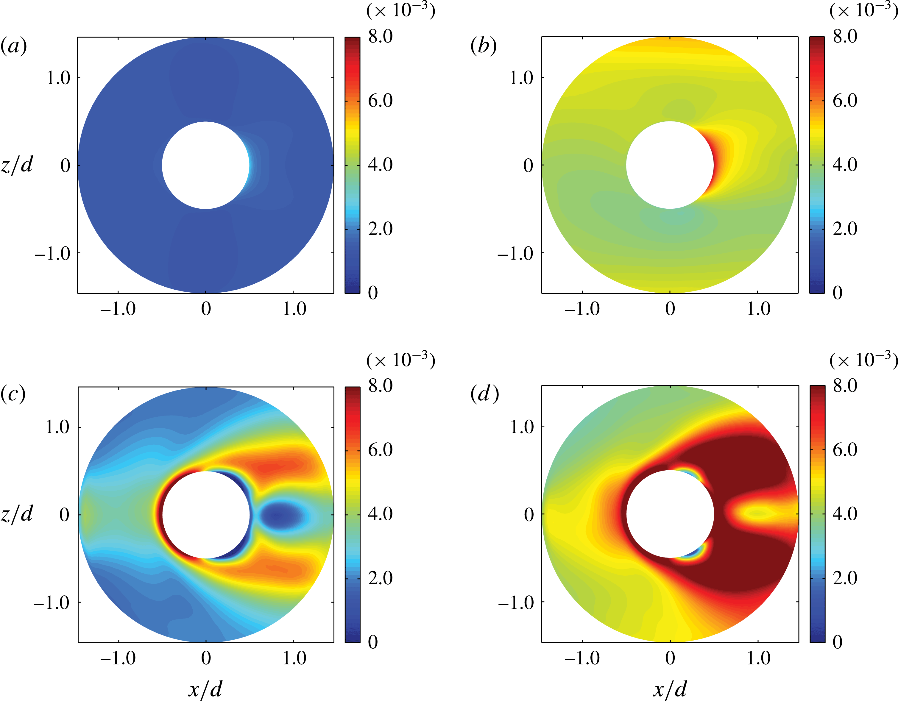
6.1 Wall shear stress
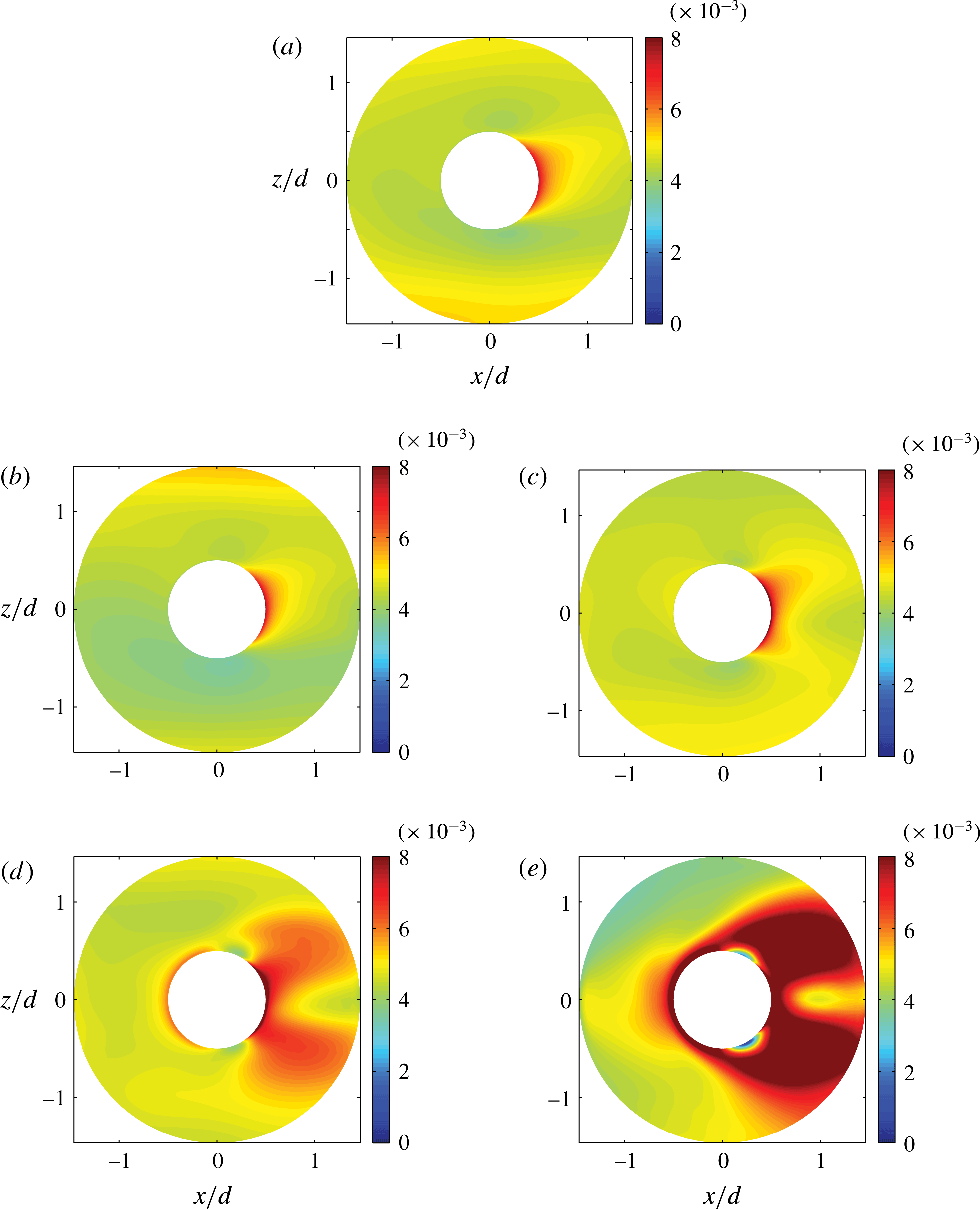
We focus first on the facesheet wall shear stress. Figure 26 shows the distribution of the time-averaged wall shear stress in the drag direction near the orifice for five cases with the orifice and cavity present. At no sound and low sound amplitude conditions the change in the wall shear stress is minimal and confined to a very small region immediately downstream of the orifice. At sound amplitudes 150 dB and above there is a noticeable increase in the wall shear stress downstream of the orifice, but also upstream of it. The latter observation is a consequence of the sound-induced pressure gradient causing the boundary layer to locally thin prior to entering the cavity. Changes to the boundary-layer state affect the change in the surface wall stress as shown in figure 27. At 130 dB incident sound amplitude the laminar boundary layer exhibits a very limited shear stress increase downstream of the orifice while at 160 dB there are two ‘wings’ of increased wall shear stress that surround a locally reversed flow region reminiscent of a jet-in-crossflow scenario (Mahesh Reference Mahesh2013).
Wall shear stress distribution with the presence of the orifice and turbulent boundary layer: (a) no sound, (b) 130 dB, (c) 140 dB, (d) 150 dB, (e) 160 dB.

Wall shear stress distribution with the presence of the orifice and laminar/turbulent boundary layer: (a) 130 dB laminar, (b) 130 dB turbulent, (c) 160 dB laminar, (d) 160 dB turbulent.

6.2 Surface drag
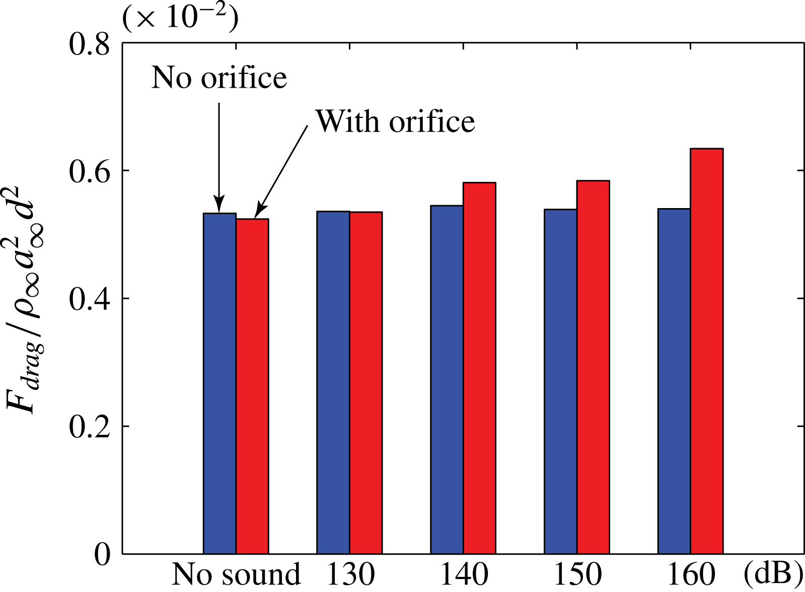
With the pointwise wall shear stress distribution evaluated with and without the presence of the orifice, we may compute the surface drag via evaluating the integrals in (6.1) and (6.2), respectively; the results are shown in figure 28. Without any incident sound the overall surface drag reduces when an orifice is punched into the facesheet, a simple consequence of the reduced surface area over which the grazing flow can generate forces. Once sound is added the facesheet drag monotonically increases. It is interesting to note that at 130 dB incident conditions, which correspond to the Langley testing conditions, the surface drag for both facesheets is approximately equal; at higher sound levels the facesheet drag increase is noticeable and on the order of 10–15 %.
Comparisons of the surface drag with and without the orifice under a turbulent boundary layer under different SPLs and 3 kHz frequency.

6.3 Total drag
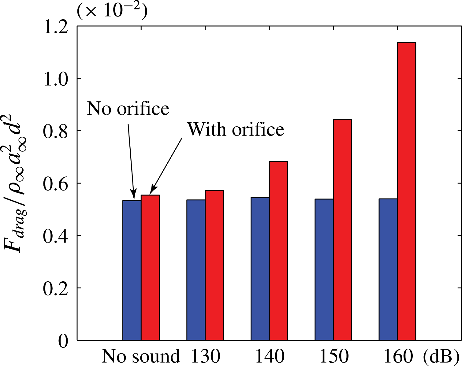
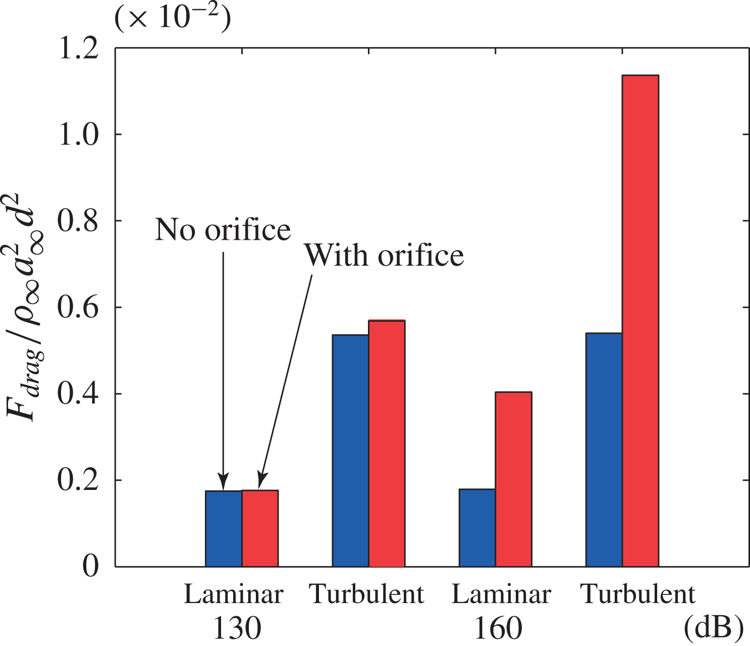
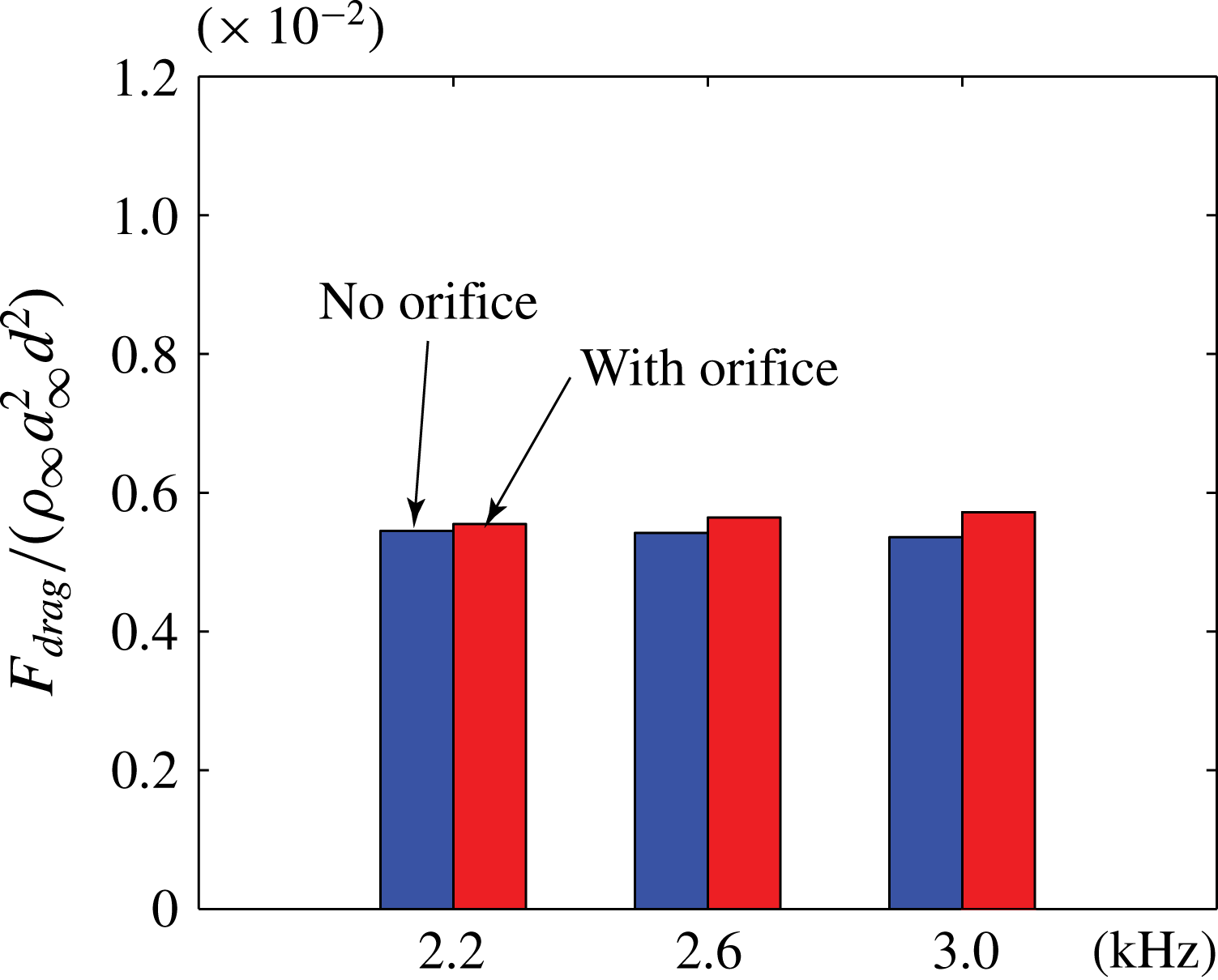
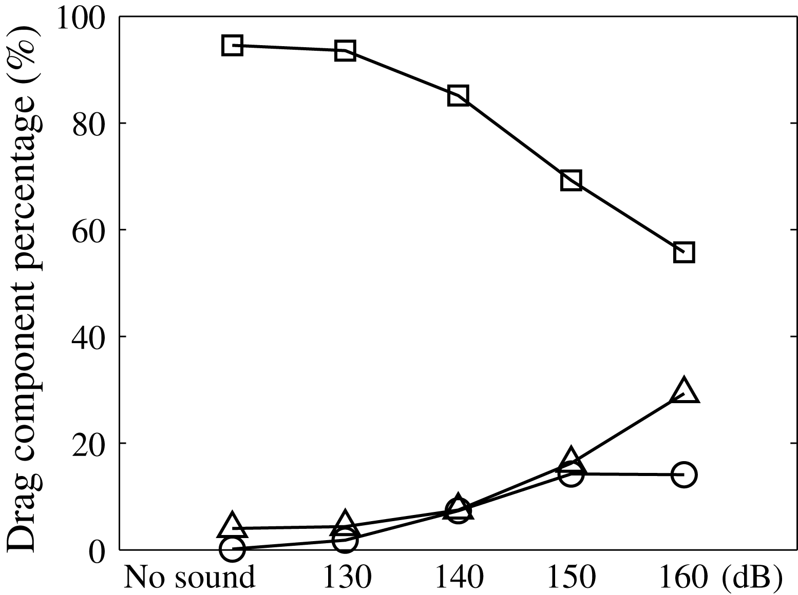
Including the cavity and orifice walls in the drag estimation in (6.2) has important consequences on the drag estimation as shown in comparing figure 29 to figure 30. With the additional surfaces the pressure forces are sufficiently large to cause a measurable drag increase for all cases, even when sound is absent, with the drag doubling at 160 dB. Important is the observation that, without sound, the surface stress only contribution shows a decrease in the drag while an increase is found when the cavity and orifice surfaces are included. This observation implies that attempts to assess linear drag using surface shear stress techniques (oil film, interferometry, in situ) only may report incorrect trends. Whether the boundary layer is laminar or turbulent changes the drag quantitatively, of course, but does not alter the general conclusions (see figure 30). Changing the incident sound frequency has a minor effect on the liner-induced drag, as shown in figure 31, but it is observed that the drag increase reduces for lower frequencies. Our database does not include frequencies lower than 2.2 kHz so we do not know whether the trend continues. Finally, figure 32 shows that as the sound amplitude increases, the cavity and orifice contribute more to the overall drag profile of the liner such that at 160 dB conditions their summation is approximately the same as the surface shear stress. If we consider the data in figures 30–32 together, it seems clear that the liner-induced drag is likely a function of sound amplitude and that surface stress measurements may not be the correct indicator.
Drag increase associated with the resonator, under a turbulent boundary layer, for 3 kHz incident sound frequency at the indicated sound amplitudes.

Drag increase associated with the resonator for 3 kHz incident sound at the indicated amplitude and boundary-layer state.

Frequency dependence of the drag increase for 130 dB incident sound and turbulent boundary layer.

Relative contributions of the facesheet (–▫–), cavity (–○–), and orifice walls (–▵–) to the drag for 3 kHz incident sound on a turbulent boundary layer.

The scaling of the drag increment is now considered using the data presented in § 5.4.1. We select case A in table 1 as the reference because there is no sound involved in which case the definition of the drag component increments become straightforward if we compute the difference between any case from set B to D with the reference case (case A),
 $$\begin{eqnarray}\displaystyle {\it\delta}F=F_{w/incidence}-F_{w/o\,incidence}. & & \displaystyle\end{eqnarray}$$
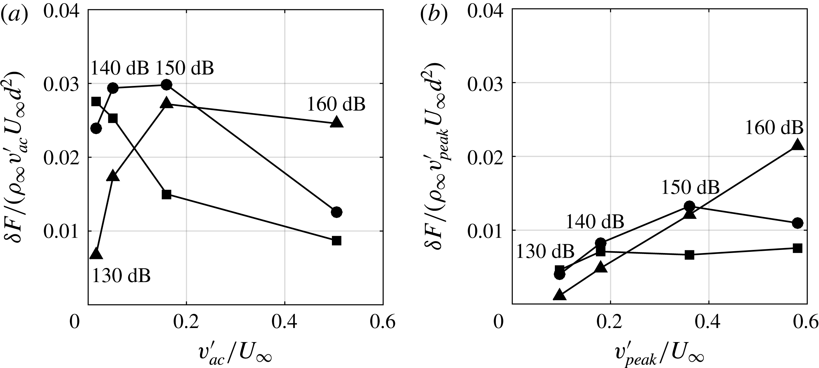
Scaling the drag increment by the velocity scales
 $v_{ac}^{\prime }$
and
 $v_{peak}^{\prime }$
introduced in § 5.4.1 are shown in figure 33. Using
 $v_{ac}^{\prime }$
(figure 33
a) yields drag increments that are only roughly constant over the 130–160 dB amplitudes investigated. Using
 $v_{peak}^{\prime }$
on the other hand, shown in figure 33(b), shows that
 ${\it\delta}F/({\it\rho}_{\infty }v_{peak}^{\prime }U_{\infty }d^{2})\rightarrow$
0.08 and 0.1 for the facesheet shear stress and cavity pressure component. The orifice wall pressure component shows a convincing quadratic scaling
 ${\it\delta}F\sim (v_{peak}^{\prime })^{2}$
and clearly indicates the importance of the hydrodynamic origin of the pressure drag.
Different drag increment component scaled by different in-orifice velocities at different SPLs. (a) Scaled by the acoustic velocity
 $v_{ac}^{\prime }$
; (b) Scaled by the simulation database
 $v_{peak}^{\prime }$
. Legends: –▪–, wall shear stress component; –●–, cavity pressure component and –▴– orifice wall pressure component (3 kHz incident sound).

7 Impedance prediction and modelling
7.1 Direct impedance prediction
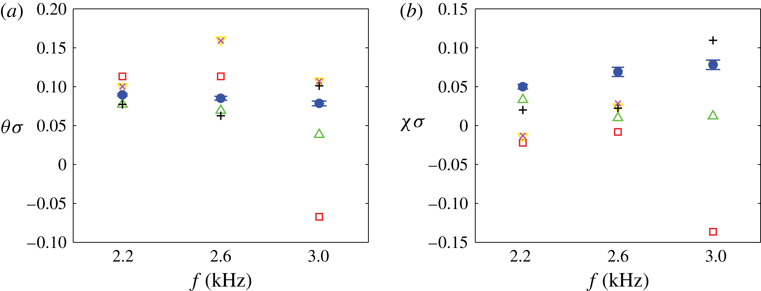
Attention now focuses on extracting the impedance values for the simulated single degree-of-freedom liner that was also tested at the NASA Langley Research Center at the same grazing flow and incident sound conditions (Jones, Watson & Nark Reference Jones, Watson and Nark2010). There are several differences between the real and simulated liner that must be mentioned. First, the porosities of the two liners are different since the experimental liner has 8–9 orifices per cavity, randomly located, while the simulated liner has only one orifice located top-dead-centre over the cavity, thus changing the porosity
 ${\it\sigma}$
from 8.7 % to 0.99 %. Under the assumption that the individual orifices do not interact (a point we will return to shortly) then a porosity-scaled impedance measure makes sense. Theoretical support for this scaling is given in Melling (Reference Melling1973), Hersh et al. (Reference Hersh, Walker and Celano2003) and in Singh & Rienstra (Reference Singh and Rienstra2014), for example, in the linear and weakly nonlinear sound amplitude regimes. Further support for the use of porosity-scaled impedance was given in Zhang & Bodony (Reference Zhang and Bodony2012) using normal impedance tube experimental data and more sophisticated semi-empirical models (Ingard Reference Ingard1953; Melling Reference Melling1973; Jones et al.
Reference Jones, Smith, Parrott and Smith2004). Note that the impedance is normalized by the characteristic impedance
 ${\it\rho}_{\infty }a_{\infty }$
.
A second difference arises because of the single orifice assumption in the simulations. The experimental liner test sample used in Jones et al. (Reference Jones, Watson and Nark2010) contained many hexagonal cavities, each with 8–9 orifices, mounted on one side of the GFIT and spatially extended in the flow direction. It stands to reason that the downstream orifices see a different environment than do the upstream orifices and, potentially, are characterized by a different impedance. The impedance eduction methods used thus represent a liner aggregate value. In contrast the simulations, with their single, isolated orifice, represent a localized value. It is not known what consequences these differences have on the values of
 $Z$
reported, but will be the focus of future studies.
The last differences are due to the idealization of the flow and acoustic environment between the GFIT and the simulations. The GFIT is a
 $2^{\prime \prime }\times 2.5^{\prime \prime }$
rectangular cross-section duct with grazing acoustic waves that have been influenced by the duct flow while the simulations assume an infinitely large facesheet with normal acoustic incidence. It is unknown how important these differences are but the results of Tam et al. (Reference Tam, Pastouchenko, Jones and Watson2014), which include duct effects and grazing incidence, suggest they are not dominant.
In addition to the physical differences in the experimental setup and conditions it is important to mention that the impedance eduction methods are also different. The simulations use a two microphone method (Dean Reference Dean1974) that connects pressure measurements taken on the liner facesheet and along the cavity end wall to estimate the local impedance that we showed to be useful when orifice effects are avoided (Zhang & Bodony Reference Zhang and Bodony2012). Using the same data collected in Jones et al. (Reference Jones, Watson and Nark2010), different hypotheses are available to link the mean flow and the pressure measurements taken within the GFIT to the estimated liner impedance. Watson and his co-workers have been examining the dependence the flow profile and eduction method has on the impedance prediction and summarized several results in Watson & Jones (Reference Watson and Jones2013) and in Jones et al. (Reference Jones, Watson, Howerton and Busse-Gerstengarbe2015) and the reader is referred to these two papers for additional details. What is relevant for the current discussion is that how the mean flow is modelled (as a plug flow or as a shear flow) and how the disturbances within the duct are modelled or approximated (as with a Pridmore–Brown equation with or without a Prony expansion) is critical to estimating the impedance.
Normalized impedance prediction at 130 dB with turbulent boundary layer. Legend: data of Jones et al. (Reference Jones, Watson and Nark2010) using different impedance eduction methods: ▫, 1-D PB model; ▵, 1-D shear flow model; ▿, 1-D PB Prony model;
 $+$
, Plug flow Prony model. The present simulation data are denoted by ●. Details on the experimental eduction methods are given in the main text. ‘PB’ is short for Pridmore–Brown: (a) normalized resistance, (b) normalized reactance.

The predicted impedance is shown in figure 34 at 130 dB tonal amplitude at the frequencies indicated and compared with the impedance values educed using different methods in Jones et al. (Reference Jones, Watson and Nark2010). It is clear that the predictions are within the scatter of impedance values educed from the experimental data and that general trends are difficult to define, at least over the modest frequency range available. (In Jones et al. (Reference Jones, Watson and Nark2010) it is noted that the cut-on frequency for the GFIT at Mach 0.5 occurs between 2.6 and 3.0 kHz so that some of the scatter present in the experimental data at 3 kHz in figure 34 may be due to the presence of these higher-order modes. The data at 2.6 kHz and below are believed to be free of high-order mode effects.) The uncertainty in the predicted values of resistance and reactance are shown by the horizontal bars visible within the symbols and indicates that the results are converged (see Zhang Reference Zhang2014).
The fact that the present impedance prediction falls within the scatter of the experimental data suggests two points. First, the simulations represent faithfully the interaction of the sound with the cavity-backed circular orifice and led credibility to the predictions. Second, and more importantly, how the impedance is educed is as important as its value since, as figure 34 shows, the scatter in
 $Z$
can exceed a factor of two and indicate opposite trends.
When simulation-only impedance predictions at a fixed frequency of 3 kHz but increasing amplitude are shown in figure 35 are considered, it is clear that whether a boundary layer is present, and its state, affects the predicted impedance to a large degree for the 130 dB sound amplitude case but very little at a sound amplitude of 160 dB. It appears to be the case that the resistance increases monotonically with increasing sound amplitude, even with a grazing flow present, and that the reactance is much less sensitive to the grazing flow, observations that are consistent with empirical modelling presented in Motsinger & Kraft (Reference Motsinger, Kraft and Hubbard1995).
Normalized impedance prediction at different SPLs and grazing flow conditions. Legend:
 $\blacklozenge$
, no grazing flow; ▪, laminar boundary layer; ●, turbulent boundary layer: (a) normalized resistance, (b) normalized reactance.

7.2 Time-domain impedance model
Our starting point is the time-domain model of the orifice-normal momentum equation studied in Zhang & Bodony (Reference Zhang and Bodony2012),
 $$\begin{eqnarray}\displaystyle {\it\rho}{\it\tau}\frac{\text{d}^{2}{\it\xi}}{\text{d}t^{2}}+{\it\rho}\frac{1-C_{D}}{C_{D}}\left|\frac{\text{d}{\it\xi}}{\text{d}t}\right|\frac{\text{d}{\it\xi}}{\text{d}t}+P_{c}S=P_{0}S\text{e}^{\text{i}{\it\omega}t}+\mathop{\sum }_{j}T_{j}S\,\text{e}^{\text{i}({\it\omega}_{j}t+{\it\phi}_{j})}, & & \displaystyle\end{eqnarray}$$
where
 ${\it\xi}(t)$
is interpreted as the orifice area-averaged displacement of the control volume at the centre point of the orifice and
 $C_{D}$
is the discharge coefficient of the orifice jet that models the effective geometry of the orifice. Further, the presence of the external turbulent boundary induces an unsteady, pseudo-random force that affects the in-orifice fluid and is modelled as the last term in the expression where
 $T_{j}$
represents the strength of the turbulent boundary-layer-induced pressure fluctuations at frequency
 ${\it\omega}_{j}$
and
 ${\it\phi}_{j}$
is the assumed-to-be random phase. We use the model of Goody (Reference Goody2004) to relate
 $T_{j}$
to the boundary-layer dynamic pressure and thickness. The cavity pressure
 $P_{c}$
is isentropically related to the change in density caused by the volume change
 $-{\it\xi}A$
.
7.3 Modelling the discharge coefficient
As we showed in the absence of a grazing flow, modelling the discharge coefficient
 $C_{D}$
in (7.1) can be reduced to modelling the in-orifice boundary layers with success (Zhang & Bodony Reference Zhang and Bodony2012). However the grazing flow creates a significant flow complexity for which we have not found a suitable fully theoretical model. We are therefore forced to use a semi-empirical approach where
 $C_{D}$
is linked to the external flow field and incident acoustic field as much as possible.
The DNS data reveals that the discharge coefficient differs significantly between the inflow and outflow cycles; therefore, it is reasonable to model them separately. Rogers & Hersh (Reference Rogers and Hersh1975), as guided by their water tunnel tests, proposed that both the inflow and outflow discharge coefficient, namely
 $C_{Di}$
and
 $C_{Do}$
, are strong functions of
 $v_{i}/U_{\infty }$
and
 $v_{o}/U_{\infty }$
, the core inflow and outflow velocities, respectively, found within the orifice, and they proposed the ‘lid model’ with a power law relation between
 $C_{D}$
and the inflow/outflow velocities. These formulas work well when
 $C_{Di}$
and
 $C_{Do}$
are small but fail when
 $v_{i}/U_{\infty }$
or
 $v_{o}/U_{\infty }$
exceed 0.3 as the expressions yield a predicted discharge coefficient greater than one. Therefore, we propose the modified parameterization,
 $$\begin{eqnarray}\displaystyle & \displaystyle C_{D_{i}}={\it\beta}_{1}\tanh \left[{\it\alpha}_{1}\left(\frac{v_{i}}{U_{\infty }}\right)^{{\it\gamma}_{1}}\right] & \displaystyle\end{eqnarray}$$
 $$\begin{eqnarray}\displaystyle & \displaystyle C_{D_{o}}={\it\beta}_{2}\tanh \left[{\it\alpha}_{2}\left(\frac{v_{o}}{U_{\infty }}\right)^{{\it\gamma}_{2}}\right], & \displaystyle\end{eqnarray}$$
 $v_{i}/U_{\infty }$
and
 $v_{o}/U_{\infty }$
goes as
 $(v_{i}/U_{\infty })^{{\it\gamma}_{1}}$
or
 $(v_{o}/U_{\infty })^{{\it\gamma}_{2}}$
when
 $v_{i}/U_{\infty }\ll 1$
or
 $v_{o}/U_{\infty }\ll 1$
. When
 $v_{i}/U_{\infty }$
and
 $v_{o}/U_{\infty }$
is large, the prediction goes to a constant,
 ${\it\beta}_{1}$
or
 ${\it\beta}_{2}$
, meaning a maximum discharge coefficient is achieved. The four parameters
 $\{{\it\beta}_{i},{\it\gamma}_{i}\}_{i=1}^{2}$
were determined from the DNS databases by using a least-squares fit informed by conditionally averaging the inflow and outflow cycles and computing the core inflow and outflow areas and by measuring the area-averaged in-orifice velocity. The results are shown in figure 36 where the present DNS data is shown alongside the original data of Rogers & Hersh (Reference Rogers and Hersh1975). The new parameterization works reasonably well and is consistent with the originally measured data.
Comparison of the measured discharge coefficient with experimental data at different
 $v_{i}/U_{\infty }$
. Legend: ○, experimental data; - - - -, empirical formula proposed by Rogers & Hersh (Reference Rogers and Hersh1975); ——, present empirical model. ▴, ▾, simulation data: (a) inflow discharge coefficient, (b) outflow discharge coefficient.

To link the discharge coefficient to the acoustic field more directly, we appeal to the phase-averaged streamlines shown in figures 15 and 16 where it is clear that the curvature of the streamlines during the inflow portion of the cycle decreases with increasing incident sound level. Assuming that the streamline curvature is a hydrodynamic effect induced by the acoustic pressure field, one can estimate from the steady Bernoulli’s equation that the induced velocity scale is,
 $$\begin{eqnarray}\displaystyle v_{i}=\sqrt{\frac{2p_{inc}^{\prime }}{{\it\rho}_{\infty }}}, & & \displaystyle\end{eqnarray}$$
where the incident sound was given in (2.9). To recover the outflow velocity
 $v_{o}$
, applying conservation of mass requires (for constant density) that,
 $$\begin{eqnarray}\displaystyle v_{i}C_{Di}=v_{o}C_{Do}, & & \displaystyle\end{eqnarray}$$
which yields an implicit equation for
 $v_{o}$
. Comparing the predicted
 $C_{D}$
values with those measured from the DNS databases is shown in figure 37 where it is seen that, to a large degree, the model performs well.
Comparison of measured (closed symbols) and modelled discharge coefficients (open symbols) for 3 kHz incident sound at the indicated amplitude.

7.4 Reduced-order model impedance prediction
The reduced-order model predictions of the liner impedance are shown in figure 38 and are compared with the educed values from the DNS databases. At 130 dB the model does a reasonable job of reproducing the qualitative trends and the quantitative values for the frequency range shown. At higher sound amplitudes the model is able to predict the resistance up to the highest amplitude case considered; however, it fails to predict the reactance accurately and exhibits a trend with increasing amplitude that is not present in the simulation data. Despite its limitations the model does properly identify the presence and state of the boundary layer in the impedance values.

8 Conclusions
Acoustic liners play an important role in reducing the noise impact of modern transport aircraft, yet little is known about the detailed fluid behaviour in and around the liner in the presence of a laminar or turbulent grazing flow. A series of direct numerical simulations of a conventional, single degree-of-freedom, locally reacting liner were thus conducted to qualitatively and quantitatively examine the flow in and around the liner orifice for several incident acoustic field parameters and laminar and turbulent boundary-layer states. The liner geometry and turbulent flow conditions correspond to test conditions examined at NASA Langley; only one orifice-cavity pair was retained to reduce the computational resource demands.
The flow within the orifice is affected by the grazing flow in two ways: the external boundary layer applies a mean shear that creates background vorticity analogous to a lid-driven cavity and imposes a velocity scale proportional to the boundary-layer friction velocity. When the grazing flow is turbulent the velocity fluctuations impose a second velocity scale proportional to the r.m.s. of the boundary-layer fluctuations. Finally, the incident sound imposes a third velocity scale that is modulated by the background vorticity. When combined these velocity scales (say,
 $\tilde{v}_{peak}$
) are able to reasonably collapse the simulation data.
Liner drag comprises a viscous component that scales linearly in
 $\tilde{v}_{peak}$
and hydrodynamic components that scale quadratically in
 $\tilde{v}_{peak}$
. At low incident sound amplitudes the viscous component dominates but becomes comparable to the hydrodynamic component at sound amplitudes expected in aircraft engine ducts, suggesting that orifice and cavity design can yield minimal drag configurations.
Vorticity magnitude of a temporal Mach 0.5 turbulent boundary layer at different time. (Coloured by the local Mach number.): (a)
 ${\it\delta}^{\dagger }/d=0.28,(U_{\infty }t)/d=0$
; (b)
 ${\it\delta}^{\dagger }/d=0.55,(U_{\infty }t)/d=350$
; (c)
 ${\it\delta}^{\dagger }/d=1.30,(U_{\infty }t)/d=758$
.

A reduced order, time-domain liner impedance model was constructed using the velocity scale
 $\tilde{v}_{peak}$
and a simulation-informed discharge coefficient model. The impedance model is sensitive to the boundary-layer state (laminar or turbulent) and thickness, as well as to the incident sound amplitude and frequency. The model performs reasonably well for the resistance but exhibits incorrect trends of reactance with increasing sound amplitude.
Acknowledgements
This work was performed under support from the Aeroacoustic Research Consortium, of the Ohio Aerospace Institute, with Ms A. Heyward and Ms C. Harmon as the technical monitors. Computational support has been provided by the National Science Foundation TeraGrid and XSEDE resources under grant TG-CTS090004. The authors are indebted to Dr M. Jones and Dr W. Watson, of the NASA Langley Research Center, for the sharing of their geometry and data, and their discussion about impedance eduction methods.
Appendix A. Simulation initialization and verification
The simulations performed in the main text are initialized as follows. The grid exterior to the facesheet, identified as grid 1 in table 2, contains the grazing boundary layer and the incident acoustic field. The initial laminar boundary layer is adapted from the compressible Blasius boundary-layer solution using the Howarth transformation (Schlichting Reference Schlichting1979) by taking the wall-normal velocity equal everywhere to zero and assuming an isothermal wall. The momentum thickness of the initial boundary layer is chosen to be smaller than the desired value of
 ${\it\delta}^{\dagger }/d\approx 2$
to give the simulation time to develop. If the boundary layer is to be laminar, no other input is needed. If the boundary layer is to be turbulent, low-amplitude instability modes are added to the initial boundary layer, following the method in Malik (Reference Malik1990), until boundary-layer transition occurs.
Snapshots of instantaneous vorticity are plotted in figure 39 at different times for a laminar-to-turbulent case. When the boundary layer reaches a thickness such that
 $Re_{{\it\delta}^{\dagger }}=2310$
, the mean turbulent velocity profile is shown in figure 40 in which the coordinates are defined as
 $y^{+}=u_{{\it\tau}}y/{\it\nu}$
and
 $u^{+}\equiv u/u_{{\it\tau}}$
, where
 $u_{{\it\tau}}\equiv \sqrt{{\it\tau}_{w}/{\it\rho}}$
. The Van Driest scaling, defined as
 $$\begin{eqnarray}\displaystyle u_{c}^{+}=\int _{0}^{U^{+}}\sqrt{\frac{\langle {\it\rho}\rangle }{{\it\rho}_{w}}}\text{d}u^{+} & & \displaystyle\end{eqnarray}$$
is used to compare our weakly compressible boundary layer to incompressible results. In the remaining part of the appendix A,
 $u_{c}^{+}$
will be written as
 $u^{+}$
unless otherwise noted. Figure 40, taken from simulation A in table 3, shows that the present DNS data matches the experimental and previous simulation data well throughout the boundary-layer height.
Semilog plot of the mean velocity profiles. Legend: ——, Present DNS data (
 $Re_{{\it\theta}}=2310$
); - - - -, simulation of Wang & Wang (Reference Wang and Wang2012) (
 $Re_{{\it\theta}}=1770$
); — ⋅ —, simulation of Wang & Wang (Reference Wang and Wang2012) (
 $Re_{{\it\theta}}=3550$
); -▵-, experiment of Degraaff & Eaton (Reference Degraaff and Eaton2000) (
 $Re_{{\it\theta}}=1430$
); -♢-, experiment of Degraaff & Eaton (Reference Degraaff and Eaton2000) (
 $Re_{{\it\theta}}=2900$
); -○-, experiment of Degraaff & Eaton (Reference Degraaff and Eaton2000) (
 $Re_{{\it\theta}}=5200$
).

Measurements of the streamwise, wall normal and spanwise stresses are plotted in figure 41(a–c) using experimental and simulation data. The Reynolds stresses are normalized by
 $u_{{\it\tau}}$
and the Van Driest transformation is again applied, viz.,
 $$\begin{eqnarray}\displaystyle \frac{\langle {\it\rho}\rangle }{{\it\rho}_{w}}\langle {u_{i}^{\prime }}^{+}{u_{j}^{\prime }}^{+}\rangle =\frac{\langle {\it\rho}\rangle \langle u_{i}^{\prime }u_{j}^{\prime }\rangle }{{\it\rho}_{w}u_{{\it\tau}}^{2}}\quad i=1,2,3. & & \displaystyle\end{eqnarray}$$
Within the sublayer there is agreement for the normal and primary shear Reynolds stress. Outside the viscous sublayer, the profiles have a strong Reynolds number dependence. For example, the
 $\langle u^{\prime +2}\rangle$
peak in the present simulation is found close to the wall and the maximum value given by the present DNS simulation is 8.06 and the location is found to be
 $y^{+}=14.05$
. According to the empirical fit for the streamwise-normal stress by Klewicki, Murray & Falco (Reference Klewicki, Murray and Falco1994), the magnitude of the peak value depends on
 $Re_{{\it\delta}^{\dagger }}$
as,
 $$\begin{eqnarray}\displaystyle \langle u^{\prime 2}\rangle _{max}=8.5\times 10^{-9}Re_{{\it\delta}^{\dagger }}^{2}+4.8\times 10^{-4}Re_{{\it\delta}^{\dagger }}^{2}+6.86, & & \displaystyle\end{eqnarray}$$
such that, for our value of
 $Re_{{\it\delta}^{\dagger }}=2310$
yields
 $\langle u^{\prime 2}\rangle _{max}=8.01$
. Furthermore, Mochizuki & Nieuwstadt (Reference Mochizuki and Nieuwstadt1996) found the peak value location of
 $\langle u^{\prime 2}\rangle _{max}$
is approximated by the expression,
 $$\begin{eqnarray}\displaystyle y^{+}(\langle u^{\prime 2}\rangle _{max})=1.7\times 10^{-4}Re_{{\it\theta}}+14.4, & & \displaystyle\end{eqnarray}$$
which yields
 $y^{+}(\langle u^{\prime 2}\rangle _{max})=14.79$
for the present DNS condition.
Profiles of Reynolds stresses normalized by the friction velocity. Legends: ——, Present DNS data (
 $Re_{{\it\theta}}=2310$
); - - - -, high-resolution LES data from Wang & Wang (Reference Wang and Wang2012) (
 $Re_{{\it\theta}}=1770$
); — ⋅ —, high-resolution LES data from Wang & Wang (Reference Wang and Wang2012) (
 $Re_{{\it\theta}}=3550$
); -▵-, experiment of Degraaff & Eaton (Reference Degraaff and Eaton2000) (
 $Re_{{\it\theta}}=1430$
); -♢-, experiment of Degraaff & Eaton (Reference Degraaff and Eaton2000) (
 $Re_{{\it\theta}}=2900$
); -○-, experiment of Degraaff & Eaton (Reference Degraaff and Eaton2000) (
 $Re_{{\it\theta}}=5200$
).

These data, plus additional comparisons shown in Zhang (Reference Zhang2014), verify that the turbulent boundary layer used in the present study is statistically consistent with expectations and fully resolved from the perspective of the velocity field. Also note that the wiggles observed in figure 41(c) is a sign of insufficient statistical convergence due to the limited data sample for a temporally growing boundary layer.
We document also the pressure field because of its importance in our acoustically driven flow. To show the correlations in terms of the streamwise and spanwise directions, the two-point autocorrelation functions of the pressure in the homogeneous
 $x$
- and
 $z$
-directions are plotted in figure 42. The figure demonstrates that the correlations of the pressure decay rapidly towards zero when
 ${\it\delta}_{x}$
or
 ${\it\delta}_{z}$
, the displacement in the
 $x$
- and
 $z$
-directions, respectively, exceeds
 $3{\it\delta}_{99}$
and
 $0.6{\it\delta}_{99}$
, confirming that the computation domain is sufficiently large to ensure decorrelation.
Correlations of density,
 $u,v,w$
velocity and pressure in
 $x$
and
 $z$
directions respectively. (
 ${\it\theta}/d=2.06$
) Legends: ——,
 $y=10y^{+}$
, - - - -,
 $y=25y^{+}$
, — ⋅ —:
 $y=53y^{+}$
. (
 $Re_{{\it\theta}}=2310$
).