2.1. Wind tunnel configuration

This study was conducted in the Virginia Tech Stability Wind Tunnel. This facility is capable of generating flow speeds up to $80~\text{m}~\text{s}^{-1}$ and has removable test sections 7.3 m long with square cross-sections of 1.83 m on edge. The anechoic test section (Devenport et al. Reference Devenport, Burdisso, Borgoltz, Ravetta, Barone, Brown and Morton2013) employed for this study, has side walls made of a stretched Kevlar fabric that contain the flow while remaining acoustically transparent. Sound passing out of these is absorbed in one of two anechoic chambers flanking the test section. The floor and ceiling of the test section are also treated to minimize acoustic reflections. Turbulence levels in the closely uniform free stream of the empty test section are 0.024 % at $30~\text{m}~\text{s}^{-1}$ and 0.031 % at $57~\text{m}~\text{s}^{-1}$ .

To grow thick high-Reynolds-number turbulent boundary-layer flows within the anechoic test section, one of the Kevlar side walls was replaced with a hard surface consisting of six modular $1.22~\text{m}\times 1.78~\text{m}$ framed Lexan panels (figure 1). The mounting arrangement allowed the position of each panel to be independently adjusted so as to form a continuous, smooth 1.78 m wide and 7.32 m long test surface with a near-zero pressure gradient.

Figure 1.

Test section configuration and coordinate system.

Figure 2.

Rough surfaces (a) square array of 1 mm radius hemispheres, (b) square array of 3 mm radius hemispheres, (c) quasi-random distribution of 3 mm radius hemispheres.

The boundary-layer flow surface was located a nominal distance of 0.1 m inside the test section side wall to make room for the adjustment hardware. A $2.4~\text{m}\times 2.4~\text{m}$ curved fairing with a smooth ABS plastic surface was used to create a gradual transition between the wind tunnel contraction and the leading edge of the surface (Morton Reference Morton2012). Boundary-layer trips were mounted on the fairing at positions 1.2 m (primary trip) and 2.1 m (forward trip) upstream of the test surface leading edge. Both trips consisted of strips of 19 mm high aluminium angle mounted with the flange oriented downstream. This arrangement produced boundary-layer thicknesses in the test section downstream of over 0.2 m.

2.2. Rough surfaces

Close-up photographs of the three rough surfaces tested are shown in figure 2. These consist of: a square array of 1 mm radius hemispheres with 5.5 mm spacing and with the rows of elements aligned with the flow direction; a scaled version of the first surface, with 3 mm hemispheres separated by 16.5 mm; a pseudo-random distribution of 3 mm surfaces with the same average element density as the second surface. (Data files containing a complete listing of the locations of all the elements in the pseudo-random surface can be obtained from the authors.) All three surfaces had the same sparseness ratio ${\it\lambda}$ of 0.052, matching Varano’s (Reference Varano2010) fetch 2. The surfaces were moulded from epoxy resin backed by paper and Kevlar, or paper and fibreglass, substrates. The 1.8 m wide and 1.2 m long moulded sections were then glued to 3 mm thick aluminium plates of the same size, designed to be bolted to the Lexan panels of the boundary-layer flow surface. The aluminium plates were shimmed to eliminate gaps or steps between adjacent sections of the rough surfaces. For the ordered surfaces, care was taken to ensure that the rows of roughness elements were aligned and contiguous between successive sections. The random surface was designed with a distribution of elements that was periodic over the 1.2 m length of each section so that there would be no interruption in the element pattern between adjacent sections. Note that the rough surfaces were only applied to the flat section of the test wall, so that each roughness fetch began 1.19 m downstream of the primary trip (figure 1). Figure 3 shows an overall view of the one of the roughness fetches (the 3 mm ordered array) installed. Both 3 mm hemispherical surfaces included close to 50 000 elements.

Figure 3.

The 3 mm ordered array of hemispheres as installed and viewed from downstream. The width of the fetch is 1.8 m. The white components in the foreground are the surface-pressure microphone holders.

2.3. Velocity instrumentation

Velocity fluctuation measurements were made in the smooth- and rough-wall boundary flows using single- and four-sensor hot-wire anemometer probes. The four-sensor probes used (Auspex Corportation model AVOP-4-100) consist of two orthogonal arrays of X-wires within a $0.75~\text{mm}^{3}$ measurement volume. This probe provides instantaneous measurement of the three components of flow velocity, with the redundant sensor reducing sensitivity to some gradient errors. Wittmer, Devenport & Zsoldos (Reference Wittmer, Devenport and Zsoldos1998) showed this type of probe to be capable of accurate Reynolds stress measurements to within 3 mm of a wall under conditions similar to those of the present study. Angle calibrations of the four-sensor probes were performed using the look-up table method of Wittmer et al. (Reference Wittmer, Devenport and Zsoldos1998). Single hot-wire probes used to provide near-wall measurements (Auspex Corporation model AHWU-100) consisted of a 1 mm-long sensor held perpendicular to the flow and parallel to the wall on a conventional arrangement of two parallel prongs.

Both single- and four-sensor probes were supported in the tunnel on a three-axis traverse gear with 0.025 mm resolution. Probes were supported from downstream on a 1 m long sting support so as to minimize any interference from the traverse. Sensors were operated in constant-temperature mode using constant-temperature anemometer bridges (Dantec Dynamics StreamLine) optimized to give a flat frequency response below 18 kHz. Anemometer signals were recorded using a 64-channel 16-bit Agilent E1432 digitizer. Probes were regularly calibrated for velocity in the wind tunnel free stream and corrected for temperature drift using the method of Bearman (Reference Bearman1971).

2.4. Pressure instrumentation

Mean wall-pressures were measured using 24 $1/4~\text{mm}$ diameter pressure taps located on the floor and ceiling of the test section bounding the boundary-layer test wall. Taps were located in rows between 0.25 and 0.36 m away from the test wall. Mean pressure data were collected using an Esterline NetScanner Model 98RK pressure scanner.

Surface-pressure fluctuations were measured using an array of five Bruel and Kjaer type 4138-A-015 1/8 in. microphones fitted with $1/2~\text{mm}$ pinhole caps. Devenport et al. (Reference Devenport, Grissom, Nathan Alexander, Smith and Glegg2011) studied the effects of pinhole size on wall-pressure fluctuations measured under a wall-jet boundary layer and found that a $1/2~\text{mm}$ pinhole was sufficient to spatially resolve pressure fluctuations within 1 to 2 dB for boundary-layer edge velocities down to well below $20~\text{m}~\text{s}^{-1}$ , the lowest speed used in the present study. A sixth B&K 4138 microphone, with a factory-provided salt and pepper cap, was used to sense the low-frequency acoustic background of the wind tunnel so it could be identified and eliminated from the signals of the other sensors.

Microphones were mounted with their caps flush (to within $\pm 0.02~\text{mm}$ ) with either the smooth wall or the substrate of each rough surface. Given Varano’s (Reference Varano2010) observations, microphones were placed as far as possible from adjacent roughness elements. For the ordered surfaces most microphone locations were therefore at the centre of a cell of four elements. The random surface design was initially selected from a number of statistically identical designs so as to avoid direct conflict between the planned microphone locations and the roughness elements. Microphones were mounted in plastic sleeves that allowed easy removal and replacement in the test wall. This allowed repeated measurements of the same flow with different microphone configurations. Microphone power, signal conditioning and data acquisition were handled using B&K Type 3050-A-060 LAN XI models which provided 24-bit simultaneous sampling at 51.2 kHz. The amplitude gain of the microphones was calibrated daily using a B&K type 4228 Pistonphone operating at 250 Hz.

Amplitude and phase response of the B&K type 4138 microphones fitted with pinholes was determined using an unaltered model 4138 microphone as a reference. Calibrations were performed in an anechoic chamber using the Agilent E1432 digitizer to generate white noise through a University Sound ID60C8 speaker. The pinhole cap produced a resonant peak in the microphone response at around 15 kHz which produced amplitude and phase variations that could be accurately fitted to the transfer function of a simple second-order system. Subsequent tests in the wind tunnel showed the shape of the resonant peak to depend on flow speed. Specifically, it was found that the damping of the response decreases with increase in Reynolds number, as the relative magnitude of the viscous effects is reduced. Microphone calibrations were therefore optimized during post-processing to account for these effects. Only adjustments to the damping were significant and then only at flow speeds above $20~\text{m}~\text{s}^{-1}$ , the largest reductions being approximately 40 % at $60~\text{m}~\text{s}^{-1}$ .

3.1. Mean pressure and velocity measurements

Measurements were made at free-stream velocities of 30 and $60~\text{m}~\text{s}^{-1}$ . Figure 4 shows the mean pressure coefficient as a function of streamwise distance $x$ for each of the different surface conditions. For all wall conditions there are slight residual favourable streamwise pressure gradients acting on the flow. The average gradient is smallest for the smooth wall, 1 mm ordered roughness and 3 mm random roughness conditions at approximately $-0.005~\text{m}^{-1}$ , and strongest for the 3 mm ordered roughness cases, at approximately double this value. The implied accelerations are mild (with $7\times 10^{-10}<-({\it\nu}/U_{e}^{2})(\text{d}U_{e}/\text{d}x)<3\times 10^{-9}$ ) but not negligible as will be discussed below.

Figure 4.

Mean pressure coefficient variation along the test wall. Smooth wall: $\,$

, $\,U_{e}=30~\text{m}~\text{s}^{-1}$ ; $\,$

,  $60~\text{m}~\text{s}^{-1}$ . 1 mm ordered roughness: ○, $30~\text{m}~\text{s}^{-1}$ ; △ $\,$ , $60~\text{m}~\text{s}^{-1}$ . 3 mm ordered roughness: $\,$

, $\,30~\text{m}~\text{s}^{-1}$ ; $\,$

, $\,60~\text{m}~\text{s}^{-1}$ . 3 mm random roughness: ⚫ $\,$ , $\,30~\text{m}~\text{s}^{-1}$ ; ▲ $\,$ , $60~\text{m}~\text{s}^{-1}$ .

Figure 5.

Mean velocity profiles, normalized on outer scales (a) and inner scales (b). See figure 4 for symbol definitions.

Mean velocity and turbulence profiles were measured for all cases at $x=6.98~\text{m}$ , close to the centrespan of the wall ( $z=0$ ). Exact spanwise locations were adjusted by a few millimetres so as to place the probes as far as possible from nearby roughness elements and avoid local element effects. With the smooth wall, mean velocity profiles measured at $z=\pm 0.153$ and $\pm 0.457~\text{m}$ were found to be almost identical to those measured at the centreline, establishing the mean two-dimensionality of the flow. A similar check on the two-dimensionality was made by examining mean velocity profiles at $x=4.7~\text{m}$ , see Forest (Reference Forest2012) and Meyers (Reference Meyers2014) for details.

Mean velocity profiles measured for the four surface conditions at two speeds, at $x=6.98~\text{m}$ , are compared in figure 5. Boundary-layer parameters determined from the mean velocity profiles are listed in table 2. The smooth wall produces a 231 mm thick boundary layer with an extensive semi-logarithmic region and momentum thickness Reynolds numbers of 35 700 and 68 700 at 30 and $60~\text{m}~\text{s}^{-1}$ . The addition of roughness, of course, increases the velocity defect near the wall and shifts the profile downward on the semi-logarithmic scale of figure 5(b). Interestingly, the defect is only slightly greater with the 3 mm than the 1 mm roughness, and the mean velocity profiles appear almost identical for the random and ordered 3 mm surfaces. Adding roughness to the flow surface caused a slight reduction in the boundary-layer thickness measured at $x=6.98~\text{m}$ (see table 2), probably reflecting a shift in the virtual origin of the boundary layer. Boundary-layer thicknesses only show slight changes with flow speed. The outer portion of the boundary-layer profiles show a somewhat weaker wake region than other measurements at high Reynolds numbers. This is a well-known effect of a favourable streamwise pressure gradient that appears even when that gradient is mild (Oweis et al. Reference Oweis, Winkel, Cutbrith, Ceccio, Perlin and Dowling2010), as in the present flows.

Table 2.

Boundary-layer parameters for the smooth and hemispherical rough surfaces at $x=7~\text{m}$ .

Skin friction coefficients for the flows were determined using the same profile-fitting method as employed by Blake (Reference Blake1970) and Aupperle & Lambert (Reference Aupperle and Lambert1970) and detailed by Schlichting (Reference Schlichting1979). This involves a two-parameter optimization of the friction velocity $U_{{\it\tau}}$ and the equivalent sand-grain roughness $k_{s}$ achieved by fitting the mean velocity profile to the form

(3.1) $$\begin{eqnarray}\displaystyle \frac{U}{U_{{\it\tau}}}=\frac{1}{{\it\kappa}}\ln \left(\frac{yU_{{\it\tau}}}{{\it\nu}}\right)-\frac{1}{{\it\kappa}}\ln \left(\frac{k_{s}U_{{\it\tau}}}{{\it\nu}}\right)+C & & \displaystyle\end{eqnarray}$$

with $C=8.5$ . The friction velocity estimates (listed in table 2) are verified in figure 6, which shows the independently measured Reynolds shear stress profiles normalized on these estimates. As would be expected, the peak values of $-\overline{uv}/U_{{\it\tau}}^{2}$ are all one, to within the scatter of the measurement.

Figure 6.

Reynolds shear stress profiles for the rough-wall boundary layers normalized on the friction velocity. See figure 4 for symbol definitions.

Examining the results in table 2 we see that friction velocity ratios $U_{{\it\tau}}/U_{e}$ are approximately 50 % larger for the rough surfaces and almost identical for the random and ordered 3 mm hemispheres. The friction velocities imply roughness Reynolds numbers $(k_{g}^{+})$ that, according to conventional criteria, suggest fully rough flows in all cases; $k_{g}^{+}$ varies from 91 for the 1 mm surface at $30~\text{m}~\text{s}^{-1}$ to 507 for the 3 mm ordered surface at $60~\text{m}~\text{s}^{-1}$ . Consistent with this, the effective sand-grain roughness is a nearly constant multiple of the geometric roughness height. Boundary-layer thickness to roughness size ratios vary from the mid-70s for the 3 mm surfaces to over 200 for the 1 mm roughness cases. All the present rough-wall flows, therefore, reach conditions at which we might expect universal scaling behaviour to become apparent.

Figure 7.

Reynolds normal stress profiles. See figure 4 for symbol definitions. Note false origins for $\overline{w^{\prime 2}}$ and $\overline{u^{\prime 2}}$ . Dashed line on the $\overline{u^{\prime 2}}$ profiles has a slope, in terms of the natural logarithm of $y^{+}$ of $-1.26$ . Dashed line over the $\overline{w^{^{\prime }2}}$ profiles has 30 % of this slope, matching the semi-logarithmic region seen by Fernholz & Finley (Reference Fernholz and Finley1996).

As already noted, a complicating factor in the concept of fully rough conditions is Mehdi et al.’s (Reference Mehdi, Klewicki and White2010, Reference Mehdi, Klewicki and White2013) argument that viscous effects should play a significant role in the boundary layer from the wall out to the Reynolds shear stress maximum. As seen in figure 6, the Reynolds stress maxima all appear well above the roughness tops, at a roughly constant absolute position of $y\cong 11~\text{mm}$ , corresponding to $y/{\it\delta}\cong 5\,\%$ and $y^{+}\cong 1000$ and 2000 at the two flow speeds. Note that this distance is comparable to the roughness spacings (of 5.5 and 16.5 mm), so the local flows around the elements may also have influenced the lower portions of the profiles, which were deliberately measured over the gaps between roughness elements.

Turbulence normal stress profiles, plotted in semi-logarithmic form, are shown for the rough-wall boundary layer cases in figure 7. The profiles show the expected dominance of $u^{\prime }$ velocity fluctuations over most of the boundary layer and the suppressed level of $v^{\prime }$ fluctuations due to the non-penetration condition at the wall. Meyers (Reference Meyers2014) shows that peak turbulence levels in the boundary layer are quite similar to those of Blake (Reference Blake1970) although those profiles, measured at significantly lower Reynolds numbers, have higher turbulence levels in the outer region. While there is some uncertainty in the $\overline{u^{\prime 2}}$ data, these profiles have a variation in the outer part of the boundary layer not inconsistent with the semi-logarithmic region seen in other high-Reynolds-number boundary-layer measurements, with a natural-logarithm slope of $-1.26$ . This is the value established by recent smooth-wall studies of Marusic et al. (Reference Marusic, Monty, Hultmark and Smits2013) and Meneveau & Marusic (Reference Meneveau and Marusic2013). The $\overline{w^{\prime 2}}$ profiles display a somewhat clearer semi-logarithmic region with a slope quite closely consistent with the highest Reynolds number measurements of Fernholz & Finley (Reference Fernholz and Finley1996), for a boundary layer at $Re_{{\it\theta}}=4736$ and a number of other smooth-wall datasets reviewed by Jiménez & Hoyas (Reference Jiménez and Hoyas2008).

Figure 8.

Microphone measurement locations. Location of the reference microphone used for acoustic background detection is indicated by the circle.

Spatial resolution of the four-sensor hot-wire probe is an important consideration in interpreting the turbulent stress results. Based on the standard established by a number of previous studies (e.g. Hutchins et al. Reference Hutchins, Nickels, Marusic and Chong2009) for the resolution of the nearest wall structure of smooth-wall boundary layers the present measurements are unquestionably under-resolved. The sensor lengths and separations in the four-sensor probes correspond to approximately 70 and 140 wall units at 30 and $60~\text{m}~\text{s}^{-1}$ , much larger than the value of 20 normally quoted as necessary for near-wall turbulence (Ligrani & Bradshaw Reference Ligrani and Bradshaw1987). However, our goal here was merely to reveal the outer form of the stress profiles including the anticipated plateau in the Reynolds shear stress. Varano (Reference Varano2010) performed an exhaustive study of skin-friction measurement methods for rough-wall turbulent boundary layers and found the measurement of the Reynolds shear stress in the plateau to be particularly accurate. The present measurements were performed starting at 3 mm from the wall, a $y^{+}$ of close to 280 and 510 at 30 and $60~\text{m}~\text{s}^{-1}$ respectively. The four-sensor probe measurements of Wittmer et al. (Reference Wittmer, Devenport and Zsoldos1998) in a fully developed pipe flow with quite similar absolute conditions to the present $30~\text{m}~\text{s}^{-1}$ experiments showed under-measurements of the Reynolds shear stress of 8 %, 4 % and 1 % at $y^{+}=300$ , 450 and 600 respectively, these last two values being smaller than the likely measurement uncertainty. If we assume this error scales with the size of the sensor, in wall units, then we would expect these errors to apply at roughly twice the $y^{+}$ values for the $60~\text{m}~\text{s}^{-1}$ cases. These errors seem likely to emphasize the roll off in the Reynolds shear stress at the lower end of the $y^{+}$ range in figure 6, but unlikely to influence the peak value and its location. We can assess the influence of probe resolution on the normal stresses using the results of Hutchins et al. (Reference Hutchins, Nickels, Marusic and Chong2009) made for a single-sensor probe. They found that sensor lengths of 79 and 153 produced under-measurement of the streamwise turbulence normal stress in the outer portions of a turbulent boundary layer at $y^{+}=280$ of approximately 6 % and 1.5 %, respectively, and at $y^{+}=540$ of approximately 3 % and 1.2 %, respectively. These errors should be borne in mind when interpreting the left-most portions of the profiles in figures 6 and 7.

3.2. Wall-pressure spectra

Microphone measurements were made at a series of positions defining streamwise and spanwise lines around $x=7~\text{m}$ , as illustrated in figure 8. Measurements were made at multiple positions to verify the homogeneity of the wall pressure field, to define streamwise and spanwise separations for the measurement of space–time correlations and, through averaging, to reduce the uncertainty in wall-pressure time spectra. Two-point correlation results, discussed in more detail by Forest (Reference Forest2012) and Meyers (Reference Meyers2014), show the correlation between boundary-layer pressure fluctuations falling to zero for spanwise separations of more than a few displacement thicknesses. Turbulent pressure fluctuations measured at the reference microphone location (marked as ○ in figure 8) were therefore independent of those measured at other microphone positions. Surface-pressure cross-spectra with the reference microphone could therefore be used to provide a measurement of the acoustic contribution to spectral levels. Significant acoustic contamination was only observed below 100 Hz, with broadband contamination not exceeding 3 dB for frequencies above 12 Hz. At frequencies where the acoustic contribution was a small fraction of the measured levels it was subtracted from those levels. Data at frequencies where the coherence between the measurement and reference microphone exceeded 0.08 were discarded.

Wall-pressure fluctuations for all the rough-surface conditions were measured at flow speeds of 20, 30, 40, 50 and $60~\text{m}~\text{s}^{-1}$ . The smooth-wall measurements were made at 22.4, 33.6, 44.8, 56.0 and $67.2~\text{m}~\text{s}^{-1}$ , the inadvertent difference being due to a mis-connected pressure transducer. Figure 9 shows absolute surface-pressure spectra measured at these conditions. Spectra are single sided and scaled to a 1 Hz bandwidth and are shown using multiple curves representing different locations along the spanwise row at $x=6.98~\text{m}$ .

Figure 9.

Pressure spectra measured at different spanwise positions at $x=6.98$  m. (a) Smooth wall: $\;$

, $\;U_{e}=22.4~\text{m}~\text{s}^{-1}$ ; $\,$

, $\,33.6~\text{m}~\text{s}^{-1}$ ; $\,$

, $\,44.8~\text{m}~\text{s}^{-1}$ ; $\,$

, $\,56~\text{m}~\text{s}^{-1}$ ; $\,$

, $\,67.2~\text{m}~\text{s}^{-1}$ . (b) 1 mm ordered surface: ▿, $\,U_{e}=20~\text{m}~\text{s}^{-1}$ ; ○, $30~\text{m}~\text{s}^{-1}$ ; ♢, $\,40~\text{m}~\text{s}^{-1}$ ; ▫, $\,50~\text{m}~\text{s}^{-1}$ ; △ , $\,60~\text{m}~\text{s}^{-1}$ . (c) 3 mm ordered surface: $\,$

, $\,U_{e}=20~\text{m}~\text{s}^{-1}$ ; $\,$

, $\,30~\text{m}~\text{s}^{-1}$ ; $\,$

, $\,40~\text{m}~\text{s}^{-1}$ ; $\,$

, $\,50~\text{m}~\text{s}^{-1}$ ; $\,$

, $\,60~\text{m}~\text{s}^{-1}$ . (d) 3 mm random surface: ▼, $\,U_{e}=20~\text{m}~\text{s}^{-1}$ ; $\,$ ⚫, $\,\text{m}~\text{s}^{-1}$ ; $\,$ ♦, $\,40~\text{m}~\text{s}^{-1}$ ; $\,$ ⬛ , $\,50~\text{m}~\text{s}^{-1}$ ; $\,$ ▲ , $\,60~\text{m}~\text{s}^{-1}$ . Vertical lines through the spectra at high frequency indicate, in each case, the frequency above which attenuation due to averaging over the pinhole would have been significant.

The results for the smooth wall (figure 9 a) display traits typical of wall-pressure spectra observed in other zero-pressure-gradient turbulent boundary-layer flows. A low signal to noise ratio limited the data at very low frequencies, though there is clear evidence of a low frequency rise for each of the spectra before reaching a shallow maximum. In the mid-frequency range after the spectral peak, a well-defined linear ‘overlap’ region is exhibited before the wall-pressure spectra begin their sharp roll-off at high frequencies due to dissipation. Data acquisition system limitations restricted the Nyquist frequency to 25.6 kHz, causing clipping of the spectral roll-off for flow speeds above $20~\text{m}~\text{s}^{-1}$ . Consistent with many previous studies (e.g. Blake Reference Blake1970; McGrath & Simpson Reference McGrath and Simpson1987; Goody Reference Goody2004) the so-called overlap region has a slope of approximately $-0.8$ and grows in frequency span as the flow speed increases. It is commonly assumed that the low slope is a transitional effect, resulting from the relatively low Reynolds number of many laboratory-scale flows. However, the high Reynolds number of the present experiments suggests that either the theoretical argument for the $-1$ slope is flawed, or the convergence to this value at high Reynolds number is extremely gradual. In the dissipation range, the spectra roll off with a slope that appears to increases rapidly with frequency. At 20 and $30~\text{m}~\text{s}^{-1}$ enough of this region is visible to see that the slope reaches, and then exceeds, the commonly stated value of $-5$ . While this type of behaviour has been seen before, both in experimental (e.g. Tsuji et al. Reference Tsuji, Fransson, Alfredsson and Johansson2007) and computational (Choi & Moin Reference Choi and Moin1990) studies, the increasingly rapid roll off here appears due to averaging effects over the microphone pinhole, as will be discussed below. As the flow speed and Reynolds number are increased, a shallow inflection appears between the ‘overlap’ and dissipation ranges, somewhat reminiscent of the bottleneck observed in the energy spectrum of homogeneous turbulence.

The pressure spectra on the rough walls have a superficially similar form to those measured on the smooth wall: a shallow maximum at low frequencies (that appears obscured by uncertainty for the 3 mm random surface), a mid-frequency region of roughly constant slope, and a rapid roll off at high frequencies with a slope that passes through and beyond $-5$ . However, a detailed comparison reveals some important differences. The spectral maximum appears at a higher absolute frequency for the same free-stream speed and, comparing the results for the 1 mm and 3 mm ordered surfaces, its frequency clearly increases with the roughness size. The mid-frequency region is less convincingly straight than with the smooth wall and has a noticeably higher slope, of approximately $-0.9$ for the 1 mm hemispherical roughness, and $-4/3$ for both 3 mm surfaces.

We would expect any effects of the slight favourable pressure gradient of the present flows on the spectrum to be most noticeable at lower frequencies where the wall-pressure spectrum contains its strongest contributions from the outer portion of the turbulent boundary layer. Schloemer (Reference Schloemer1967) made measurements of the effects of favourable pressure gradient on the wall-pressure fluctuations of a smooth-wall boundary layer for an acceleration parameter $K=3.3\times 10^{-7}$ more than two orders of magnitude greater than those of the present flows. Schloemer’s data were further analysed by Cipolla & Keith (Reference Cipolla and Keith2000) who found that, when scaled on outer variables, the wall-pressure fluctuations in the favourable-pressure-gradient boundary layer were suppressed at frequencies ${\it\omega}{\it\delta}/U_{e}\lesssim 3$ , corresponding to dimensional frequencies in the present flows of approximately 40 Hz at $20~\text{m}~\text{s}^{-1}$ increasing to approximately 130 Hz at $60~\text{m}~\text{s}^{-1}$ . This encompasses the region in the immediate vicinity of the low-pressure maximum. This could explain, at least for the smooth-wall case, why the roll off from the maximum is rounded and involves a continuous increase in slope magnitude with frequency. Pressure spectra measured by some authors (e.g. Klewicki et al. Reference Klewicki, Priyadarshana and Metzger2008) show a more pronounced maximum that is also present in Panton & Linebarger’s (Reference Panton and Linebarger1974) smooth-wall spectral model. However, this feature does not appear to be universal to smooth-wall boundary layers as can be seen in the data sets reviewed by Goody (Reference Goody2004) and, indeed, Goody’s model does not include this feature.

A close examination of the results for the 3 mm ordered and random rough surfaces (figure 9 c,d) show them to be nearly identical in all significant details. An overlaid comparison of streamwise-averaged spectra show differences of 2 dB or less in the spectral level at $20~\text{m}~\text{s}^{-1}$ , with pressure fluctuations for the random distribution of roughness elements generally being weakest. This difference disappears as the flow speed is increased.

The spanwise uniformity of the pressure fluctuation field, as revealed by the spread of the curves shown at each flow speed in figure 9, appears quite good for the smooth-wall flow. With the roughness, there is more variation at higher frequencies, presumably because of slight differences in the effects of local roughness elements. Pressure spectra measured at different streamwise positions in the array show a comparable level of similarity, suggesting near homogeneous flow in planes parallel to the wall. Therefore, wall-pressure spectra presented in later sections are averaged across the microphone locations.

It is well known that the finite size of a microphone pinhole can have a significant impact on the measurement of the highest-frequency pressure fluctuations. Perhaps the most definitive studies are those due to Schewe (Reference Schewe1983) and Gravante et al. (Reference Gravante, Naguib, Wark and Nagib1998). Schewe examined pressure fluctuations under a turbulent boundary layer using five microphones with pinholes with diameters $d$ between 1 and 18 mm ( $d^{+}=dU_{{\it\tau}}/{\it\nu}=19{-}333$ ). He concluded that a diameter of no more that $d^{+}=20$ was needed to completely resolve the pressure fluctuations, though his data showed that results from larger pinholes could be corrected using the method of Corcos (Reference Corcos1963, Reference Corcos1967), to some extent. Gravante et al. (Reference Gravante, Naguib, Wark and Nagib1998) performed a similar study but with a set of smaller microphones of $d^{+}=4{-}27$ . They conclude that having $d^{+}\leqslant 18$ avoids spectral attenuation for frequencies up to $f^{+}=f{\it\nu}/U_{{\it\tau}}^{2}=1$ .

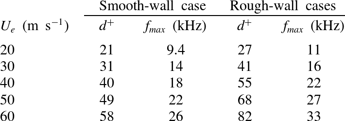
Schewe (Reference Schewe1983) and Gravante et al. (Reference Gravante, Naguib, Wark and Nagib1998) achieved the low values of $d^{+}$ they needed in part by studying slow-speed flows ( $16~\text{m}~\text{s}^{-1}$ or less) where the viscous scale is large. At the higher speeds demanded by the requirements of high Reynolds number, achieving such $d^{+}$ values implies pinhole diameters that (at least with the present microphones) would be incompatible with maintaining a sufficient frequency response. The present microphone system therefore under-resolves the highest-frequency pressure fluctuations. However, we can use the results of Gravante et al. (Reference Gravante, Naguib, Wark and Nagib1998) and Schewe (Reference Schewe1983) to estimate the frequencies at which that attenuation would have become significant. Table 3 lists $d^{+}$ for the 0.5 mm pinholes used in the present experiments as functions of flow speed and surface. Gravante et al.’s (Reference Gravante, Naguib, Wark and Nagib1998) results include a case, with $d^{+}\approx 26$ , where the pressure spectrum was under-resolved. In this case the measured spectral levels were within 2 dB of the true levels up to a frequency $f^{+}\approx 2.2$ . We can use this result to estimate the maximum useful frequency measured by the current microphones by assuming that this frequency varies inversely with $d^{+}$ . If anything, Schewe’s (Reference Schewe1983) results, which include a sequence of spectra measured with increasingly under-resolved transducers, suggest that this is a pessimistic estimate. High-frequency limits on the present measurements estimated using this method are included in table 3 and shown graphically with the vertical lines in figure 9. These limiting frequencies lie only within the measured frequency range (up to 25 kHz) at flow speeds of $30~\text{m}~\text{s}^{-1}$ or less ( $40~\text{m}~\text{s}^{-1}$ for the smooth wall). At these speeds the limits come in the middle of the dissipation range and largely clip the portion of the spectrum that rolls off with a slope greater than $-5$ , at least for the smooth wall condition. Data above the limiting frequencies are not included in subsequent figures.

Table 3.

Diameter of the 0.5 mm microphone pinhole expressed in wall units, and frequency limits on wall-pressure fluctuation measurements estimated using the results of Schewe (Reference Schewe1983) and Gravante et al. (Reference Gravante, Naguib, Wark and Nagib1998).

3.3. Scaling of the pressure spectrum

The applicability of various scaling suggestions made by previous researchers are examined in this section. We consider not only their applicability to the different rough-surface flows of the present experiments, but also the extent to which they correlate the present results to those of the previous studies listed in table 1, where the boundary layer to roughness size ratios were not as large, but which represent a range of sparseness ratios and roughness geometries.

Figure 10.

Pressure spectra measured scaled using outer variables. Mixed outer scaling, present data (a) and with results from prior studies (b). Classical outer scaling, present data (c) and with results from prior studies (d). Symbols for present data given in figure 4. $\,$

, Varano (Reference Varano2010) fetch 1, $27~\text{m}~\text{s}^{-1}$ ; $\,$

, $\,20~\text{m}~\text{s}^{-1}$ ; ◁ , fetch 2, $\,27~\text{m}~\text{s}^{-1}$ ; ▷ , $\,20~\text{m}~\text{s}^{-1}$ ; $\,$

 , fetch 3, $\,27~\text{m}~\text{s}^{-1}$ ; $\,$

, $\,20~\text{m}~\text{s}^{-1}$ ; $~$ ◀ , fetch 4, $\,27~\text{m}~\text{s}^{-1}$ ; $~$ ▶ , $\,20~\text{m}~\text{s}^{-1}$ ; $\,$

, Blake (Reference Blake1970) D-L, $38~\text{m}~\text{s}^{-1}$ ; $\,$

, $\,50~\text{m}~\text{s}^{-1}$ ; $\,$

S–S, $\,38~\text{m}~\text{s}^{-1}$ ; $\,$

, $\,50~\text{m}~\text{s}^{-1}$ ; $\,$

D–S, $\,38~\text{m}~\text{s}^{-1}$ ; $\,$

, $\,50~\text{m}~\text{s}^{-1}$ .

We begin with the low-frequency portion of the spectrum which is expected to scale on outer variables. Many different scalings were tried for this region, the best of which are shown in figure 10. Figure 10(a) shows the ‘mixed’ scaling used by Blake (Reference Blake1970), ${\it\phi}({\it\omega})U_{e}/{\it\tau}_{w}^{2}{\it\delta}^{\ast }$ versus ${\it\omega}{\it\delta}^{\ast }/U_{e}$ , applied to the present measurements. This scaling correlates all the spectra measured on the smooth and rough walls, and at different speeds, to within approximately $\pm 1.5~\text{dB}$ for frequencies up to ${\it\omega}{\it\delta}^{\ast }/U_{e}\approx 4$ , well beyond the spectral peak. Adding the data from previous studies (excluding the data of Aupperle & Lambert Reference Aupperle and Lambert1970, which show no low-frequency maximum) results in a somewhat less convincing plot (figure 10 b). Spectra still correlate best near the peak, but are spread over a band some 6–7 dB wide from ${\it\omega}{\it\delta}^{\ast }/U_{e}\approx 2$ to $4$ . However, approximately half of the scatter in this band is due to Varano’s (Reference Varano2010) data, most of which lie above the present measurements, and those of Blake (Reference Blake1970), and do not collapse well within themselves when normalized in this way. Varano himself noted this lack of collapse at low frequency and attributed it to the merger of the outer portion of his boundary layer with the boundary layer growing on the opposite wall of the channel in which his experiments were performed.

Shown in figure 10(c,d) is the ‘classical’ low-frequency scaling used for smooth-wall boundary-layer pressure spectra by Farabee & Casarella (Reference Farabee and Casarella1991) and Goody (Reference Goody2004), ${\it\phi}({\it\omega})U_{{\it\tau}}/{\it\tau}_{w}^{2}{\it\delta}$ versus ${\it\omega}{\it\delta}/U_{{\it\tau}}$ . This produces almost identical results to those of the mixed scaling, closely correlating the low-frequency portions of the present smooth- and rough-wall pressure spectra approximately in the range $20\lesssim {\it\omega}{\it\delta}U_{{\it\tau}}\lesssim 800$ (figure 10 c). We see in figure 10(d) that this scaling also does quite well in correlating the present low-frequency results to those of Blake (Reference Blake1970) but, as with the mixed scaling, leaves Varano’s data above these data sets. Even though the mixed and classical outer scalings perform comparably, we believe that the classical scaling should be preferred since it is more fundamental and physically justifiable, depending on a distance scale $({\it\delta})$ directly experienced by the flow rather than one implied by its mean profile. We therefore conclude that, of the normalizations considered, the classical scaling is most likely to describe the low-frequency behaviour of rough-wall turbulent boundary-layer pressure spectra.

Other low-frequency scalings attempted included normalizing the spectra using only boundary-layer edge scales, i.e. ${\it\phi}({\it\omega})U_{e}/({\it\rho}U_{e}^{2})^{2}{\it\delta}$ versus ${\it\omega}{\it\delta}/U_{e}$ . This was found to better align the low-frequency portions of Varano’s (Reference Varano2010) spectra with the other rough-wall data but displaces all the rough-wall results approximately 8 dB above those for smooth walls in this range, a result incompatible with the expectation that the true low-frequency scaling should unite the low-frequency behaviour of both smooth- and rough-wall boundary layers. A similar result (collapse of the low-frequency portions of the smooth and rough-wall spectra onto different curves) was seen with the normalization ${\it\phi}({\it\omega})U_{e}/({\it\rho}U_{e}U_{{\it\tau}})^{2}{\it\delta}$ versus ${\it\omega}{\it\delta}/U_{e}$ inspired by DeGraaff & Eaton’s (Reference DeGraaff and Eaton2000) scaling for streamwise velocity fluctuations in smooth-wall boundary layers at high Reynolds numbers. Normalizations were also constructed using the hybrid scale $\sqrt{{\it\delta}{\it\nu}/U_{{\it\tau}}}$ discussed by Klewicki et al. (Reference Klewicki, Fife and Wei2009) and associated with the pressure-centre of (smooth-wall) boundary layers. Despite its uncertain applicability to rough-wall flows, using this in place of ${\it\delta}$ in the classical scaling produced a collapse of the present rough-wall spectra with those of Blake (Reference Blake1970) and Varano (Reference Varano2010) slightly better than that achieved with the mixed scaling (figure 10 a). However, correlation between rough- and smooth-wall flows was not quite as good as with the mixed or classical scalings.

We now turn our attention to examining the so-called ‘inner scaling’ for the rough-wall data. Blake (Reference Blake1970) first argued that the pressure fluctuations generated from the inner portion of the boundary layer should scale as ${\it\phi}({\it\omega})U_{{\it\tau}}/({\it\tau}_{w}^{2}k_{g})$ versus ${\it\omega}k_{g}/U_{{\it\tau}}$ at high frequency. Note that the frequency scale ${\it\omega}k_{g}/U_{{\it\tau}}$ is essentially the roughness Strouhal number. Aupperle & Lambert (Reference Aupperle and Lambert1970) considered a similar scaling using the effective sand-grain roughness height $k_{s}$ instead of $k_{g}$ , and with the spectral level additionally normalized on $C_{f}$ , i.e. ${\it\phi}({\it\omega})U_{{\it\tau}}/{\it\tau}_{w}^{2}k_{s}C_{f}$ versus ${\it\omega}k_{s}/U_{{\it\tau}}$ .

Figure 11.

Pressure spectra scaled using previously proposed inner-variable scalings. Blake scaling, present data (a) and with results from prior studies (b). Aupperle and Lambert scaling, present data (c) and with results from prior studies (d). Aupperle and Lambert; $\,$

, grade 36; ⨯ , grade 12; $\,$

, grade 4. Other symbols given in figure 10.

Figure 12.

Pressure spectra scaled using roughness scalings. Varano scaling, present data (a) and with results from prior studies (b). Scaling based on Mehdi et al.’s (Reference Mehdi, Klewicki and White2013) hybrid roughness/boundary layer thickness scale $\sqrt{k_{s}{\it\delta}}$ , present data (c) and with results from prior studies (d). Symbols given in figure 11.

Figure 11(a) depicts Blake’s scaling using data from the present study. This clearly does not collapse the highest-frequency portions of the pressure spectra as there is a vast variation here across test speeds and configurations. Figure 11(b) shows the same data with the added studies of Aupperle & Lambert (Reference Aupperle and Lambert1970), Blake (Reference Blake1970) and Varano (Reference Varano2010). Similar lack of performance is seen with Aupperle & Lambert’s scaling applied to data from the present study in figure 11(c), and to all the data sets in figure 11(d).

Although Blake’s scaling fails at the highest frequencies, it does show some clear signs of collapsing the spectra in the mid-frequencies $3<{\it\omega}k_{g}/U_{{\it\tau}}<20$ where it aligns the spectra so that they group into a single narrower band whose overall slope is around $-4/3$ . Looking at just the present data, figure 11(a), which combine the largest roughness Reynolds numbers and largest boundary-layer thickness to roughness size ratios, the collapse is particularly good, and to within approximately $\pm 1~\text{dB}$ . The correlation using Blake’s scaling is less clear when all the data sets are included as shown in figure 11(b), but is better than that produced by Aupperle & Lambert’s scaling, see figure 11(d).

Recently Varano (Reference Varano2010) proposed another so-called inner variable scaling. Starting with Blake’s scaling, Varano argued that for fully rough flows the friction velocity should be proportional to the edge velocity. If replaced, one obtains the scaling ${\it\phi}({\it\omega})/({\it\rho}^{2}U_{e}^{3}k_{g})$ versus ${\it\omega}k_{g}/U_{e}$ . Varano’s scaling is applied to the pressure spectra for the present study in figure 12(a). This scaling also fails at high frequencies but is perhaps the most successful in collapsing the mid-frequency region $0.06<{\it\omega}k_{g}/U_{e}<1$ . Varano’s scaling also produces the best mid-frequency correlation between the present data and the spectra of Blake and Varano, but is unable to scale Aupperle & Lambert’s results, figure 12(b).

A number of normalizations derived from the distance scales for rough-wall boundary layers proposed by Mehdi et al. (Reference Mehdi, Klewicki and White2010) were considered. Figure 12(c,d) shows the scaling ${\it\phi}({\it\omega})U_{{\it\tau}}/{\it\tau}_{w}^{2}\sqrt{k_{s}{\it\delta}}$ versus ${\it\omega}\sqrt{k_{s}{\it\delta}}/U_{{\it\tau}}$ , based on the hybrid roughness/boundary-layer thickness scale $\sqrt{k_{s}{\it\delta}}$ . Looking only at the present data (figure 12 c), this scaling appears to work particularly well at the low-frequency end of the $-4/3$ region and provides a measure of collapse around the spectral maximum, perhaps not surprising as it is the geometric average of the classical outer region and Blake scalings. This formulation does not do well in correlating the present results with other data sets, however, as shown in figure 12(d).

With the benefit of hindsight, it is perhaps not surprising that Blake’s, Aupperle & Lambert’s and Varano’s scalings do not work at the highest frequencies since none of them contains any direct reference to viscosity. Even in a high-Reynolds-number rough-wall flow one would expect viscosity to ultimately control the smallest turbulent scales and thus the highest-frequency pressure fluctuations. Indeed, the discussion of Mehdi et al. (Reference Mehdi, Klewicki and White2010, Reference Mehdi, Klewicki and White2013), referenced above, suggest that viscous effects may remain a substantial player in the dynamics of the near-wall region to a position well above the roughness tops, to the vicinity of the maximum in the Reynolds shear stress profile.

With the likely importance of viscosity to the high-frequency pressure fluctuations in mind, Forest (Reference Forest2012) postulated that a meshing of time scales was needed in order to scale the high-frequency pressure spectra. The scaling ${\it\nu}/u_{{\it\tau}}^{2}$ is based in the viscous time scale for the wall bounded flow, whereas Blake’s scaling $k_{g}/u_{{\it\tau}}$ reflects the time scale for the roughness elements. Forest argued that even for fully rough flows, both time scales may still influence the near-wall turbulent structures. This led him to take the geometric average of both time scales, yielding a scaling of the form ${\it\phi}({\it\omega})U_{{\it\tau}}/{\it\tau}_{w}^{2}\sqrt{{\it\nu}k_{g}/U_{{\it\tau}}}$ versus ${\it\omega}\sqrt{{\it\nu}k_{g}/U_{{\it\tau}}}/U_{{\it\tau}}$ , along with a similar scaling using the effective sand-grain roughness $k_{s}$ . Mehdi et al. (Reference Mehdi, Klewicki and White2010) independently introduced the length scale $\sqrt{{\it\nu}k_{s}/U_{{\it\tau}}}$ as potentially important in describing the flow between the roughness tops and the Reynolds stress maximum. Figure 13(a) shows Forest’s scaling applied to the data of the present study. It provides a marked improvement at the highest frequencies compared to the above formulations that do not include viscosity. However, it is unable to completely correlate the results for the 1 and 3 mm roughness cases, if only because the mid- and high-frequency portions of those spectra have different shapes. Adding the data from other studies produces the plot shown in figure 13(b). Overall Forest’s (Reference Forest2012) formulation seems to provide the best compromise in scaling the right-hand portions of these spectra, given that the differing spectral shapes here preclude any exact single scaling. Note that using $k_{s}$ in this scaling in place of $k_{g}$ appeared to make no significance difference to the results.

Figure 13.

Pressure spectra normalized using Forest’s (Reference Forest2012) scaling. Present data (a) and with results from prior studies (b). Symbols given in figure 11.

3.4. A new scaling for the highest-frequency pressure fluctuations

In this section we address the possibility of scaling the highest-frequency portion of the pressure spectrum, namely the region of rapid rolloff where the slope of the spectrum is seen to reach $-5$ . This region, clearly visible in the present measurements plotted in figure 9(b–d), bears more than a passing resemblance to the viscous dissipation region seen in the smooth-wall pressure spectra of figure 9(a). It is therefore tempting to suggest that both rough- and smooth-wall spectra follow a Kolmogorov-type scaling in this region. We therefore revisit the smooth-wall viscous scaling ${\it\phi}({\it\omega})U_{{\it\tau}}^{2}/({\it\tau}_{w}^{2}{\it\nu})$ versus ${\it\omega}{\it\nu}/U_{{\it\tau}}^{2}$ , which is applied to the present rough- and smooth-wall data in figure 14(a). Normalized in this way, the high-frequency portions of the smooth-wall spectra collapse onto the same curve. The same is not seen for the rough-wall spectra, though, each of which roll off at widely separated normalized frequencies and levels. The rough-wall spectra are not totally unorganized, however, as the normalized roll off frequency is seen to increase consistently as the Reynolds number is reduced for each rough surface.

Figure 14.

Pressure spectra scaled using viscous scales with (a) the conventionally defined friction velocity (present data), (b) the shear friction velocity (present data), and (c) the shear friction velocity (all datasets). Symbols given in figure 11.

While the smooth-wall viscous scaling in its unmodified form does not come even close to collapsing the highest-frequency portion of the rough-wall pressure spectra, the viscous-like behaviour of this part of the spectrum leads us to propose a scaling of the form ${\it\phi}({\it\omega})U_{{\it\nu}}^{2}/({\it\tau}_{{\it\nu}}^{2}{\it\nu})$ versus ${\it\omega}{\it\upsilon}/U_{{\it\nu}}^{2}$ , where $U_{{\it\nu}}$ is a modified friction velocity and ${\it\tau}_{{\it\nu}}=U_{{\it\nu}}^{2}{\it\rho}$ is the corresponding wall shear stress. We will refer to $U_{{\it\nu}}$ as the ‘shear friction velocity’. For a smooth wall we take $U_{{\it\nu}}$ as equal to the conventionally defined friction velocity. For a rough wall we choose the value of $U_{{\it\nu}}$ so that the high-frequency portion of the normalized spectrum matches that for the smooth wall, as nearly as possible. It is important to note that there is no a priori reason to believe that such a match can be made since the positioning of the scaled spectrum has two degrees of freedom, and the choice of $U_{{\it\nu}}$ provides only one adjustment.

Nevertheless, it was found that values of $U_{{\it\nu}}$ could be chosen to accurately collapse the high-frequency portions of all the current rough-wall pressure spectra as illustrated in figure 14(b). Using the same procedure it was found that values of $U_{{\it\nu}}$ could be chosen for Varano’s (Reference Varano2010), Blake’s (Reference Blake1971) and Aupperle & Lambert’s (Reference Aupperle and Lambert1970) rough-wall pressure spectra that would likewise correlate the roll off regions. Figure 14(c) shows the resulting normalized spectra, all of which collapse to a narrow band just a few dB wide in this region for non-dimensional frequencies ${\it\omega}{\it\nu}/U_{{\it\nu}}^{2}$ greater than approximately 0.5 displaying, together, a clear $-5$ slope at the highest frequencies.

Values of $U_{{\it\nu}}$ used to collapse the rough-wall pressure spectra are listed in table 4 and plotted in figure 15. The ratio of the shear friction velocity $U_{{\it\nu}}$ to the conventional friction velocity $U_{{\it\tau}}$ exhibits consistent trends when plotted against roughness Reynolds number $k_{g}^{+}=U_{{\it\tau}}k_{g}/{\it\nu}$ , as shown in this figure. We see that for all the rough surfaces $U_{{\it\nu}}/U_{{\it\tau}}$ is less than one. For the present data, representing three rough surfaces with a sparseness ${\it\lambda}=0.052$ , this ratio decreases monotonically with increasing roughness Reynolds numbers starting at 0.75 for the $20~\text{m}~\text{s}^{-1}$ flow over 1 mm hemispheres $(k_{g}^{+}=62)$ and dropping to 0.58 for $60~\text{m}~\text{s}^{-1}$ flows over the two 3 mm hemisphere surfaces $(k_{g}^{+}\cong 500)$ . Together the variations for the three rough surfaces define a single curve. Also included in figure 15 and table 4 are values inferred from the measured spectra of other studies. These values are more scattered but, at the same time, represent a range of sparseness values. Values of $U_{{\it\nu}}/U_{{\it\tau}}$ for Varano’s (Reference Varano2010) experiments ( ${\it\lambda}=0.013$ , 0.025, 0.052 and 0.098) are rather scattered, but overall show a decrease as the roughness becomes more dense and the sparseness ratio is reduced. Although Blake (Reference Blake1970) did not give precise sparseness ratios for his surfaces, exactly the same trend is visible in the data obtained from his spectra, with the S-S (sparse-small) rough surface being associated with significantly larger values of $U_{{\it\nu}}/U_{{\it\tau}}$ than either of the dense roughness surfaces, D-S and D-L. Values of $U_{{\it\nu}}/U_{{\it\tau}}$ for Aupperle & Lambert’s (Reference Aupperle and Lambert1970) spectra stand apart from those of other experiments, being somewhat low and showing a gradually increasing trend with $k_{g}^{+}$ .

Figure 15.

Shear friction velocities. Values inferred from pressure spectra: $\,$

1 mm hemispheres; $\,$

, 3 mm hemispheres (ordered); $\,$

, 3 mm hemispheres (random); $\,$

, Varano (Reference Varano2010), fetch 1; $\,$

, fetch 2; $\,$

 , fetch 3; $\,$

, fetch 4; ⨯ , Blake (Reference Blake1970) S–S; $\,$

, D–S; $\,$

, D–L; $\,$

, Aupperle & Lambert (Reference Aupperle and Lambert1970). Open symbols for the present experiments show estimates obtained using (3.3).

Table 4.

Values of $U_{{\it\nu}}/U_{{\it\tau}}$ determined by spectral fitting.

3.5. Physical interpretation of the shear friction velocity

A possible explanation of the above results is that viscous scales contributing to the pressure fluctuations at the wall, at locations not immediately adjacent to roughness elements, scale like those of a smooth-wall boundary layer ${\it\omega}{\it\nu}/U_{{\it\tau}}^{2}$ but with a friction velocity calculated without the contribution from the pressure drag on the roughness elements. This is consistent with the ratio $U_{{\it\nu}}/U_{{\it\tau}}$ being less than one for all rough surfaces, with it decreasing with roughness Reynolds number as the pressure drag on roughness elements increases, and with it increasing with the sparseness ${\it\lambda}$ and thus the proportion of the wall that is smooth.

Starting with this interpretation it is possible to write down a relationship between $U_{{\it\nu}}$ , $U_{{\it\tau}}$ , the sparseness ratio and the drag coefficient of the roughness elements. The overall wall shear stress ${\it\tau}_{w}$ can be broken down into the average drag force on each roughness element $D$ , and the averaged substrate wall shear stress ${\it\tau}_{{\it\nu}}$ for which the element drag is excluded:

(3.2) $$\begin{eqnarray}{\it\tau}_{w}={\it\tau}_{{\it\nu}}+nD,\end{eqnarray}$$

where $n$ is the number of roughness elements per unit planform surface area. It can be noted that while the drag force $D$ includes both pressure and viscous forces, the viscous contributions are expected to be relatively minor, while the averaged substrate wall shear stress ${\it\tau}_{{\it\nu}}$ is entirely composed of the viscous forces acting along the wall. Following Schlichting (Reference Schlichting1979), we assume that a particular roughness element can be usefully thought of as having a fixed drag coefficient $C_{D}=D/\bar{q}A$ , where $A$ is the frontal projected area of the roughness element and $\bar{q}$ is the dynamic pressure averaged over the height of the element. Recognizing that the sparseness ratio ${\it\lambda}=nA$ and the shear friction velocity $U_{{\it\nu}}=\sqrt{{\it\tau}_{{\it\nu}}/{\it\rho}}$ we obtain

(3.3) $$\begin{eqnarray}U_{{\it\tau}}^{2}=U_{{\it\nu}}^{2}+{\it\lambda}C_{D}\bar{q}/{\it\rho}.\end{eqnarray}$$

Note that in the case of the smooth wall equation (3.3) reduces to $U_{{\it\tau}}^{2}=U_{{\it\nu}}^{2}$ , since there are no roughness effects to account for.

To test the credibility of our physical interpretation, we have used (3.3) to estimate $U_{{\it\nu}}/U_{{\it\tau}}$ for the hemispherical roughness cases of the present measurements. For this purpose we roughly approximate the value of $\bar{q}$ by using a one-seventh power-law profile $U/U_{e}=(y/{\it\delta})^{1/7}$ to give

(3.4) $$\begin{eqnarray}\bar{q}=\frac{1}{2}{\it\rho}U_{e}^{2}\frac{1}{k_{g}}\int _{0}^{k_{g}}\left(\frac{y}{{\it\delta}}\right)^{2/7}\text{d}y=\frac{7}{18}{\it\rho}U_{e}^{2}\left(\frac{k_{g}}{{\it\delta}}\right)^{2/7}.\end{eqnarray}$$

This, of course, ignores the profile dependence on viscous and roughness scales. Since the boundary-layer thickness, edge velocity, friction velocity and roughness size are known, it is then only necessary to select the value of $C_{D}$ to make a prediction. Generally speaking one would expect the drag coefficient to be a function of the roughness element shape, Reynolds number, and spacing, and thus a variable in (3.3). However, we are able to obtain reasonable estimates of the shear to friction velocity ratios for the present hemispherical roughness cases by choosing a constant drag coefficient of 0.26, see figure 15. This value is quite close to the drag measurement of Bennington (Reference Bennington2004), implying $C_{D}=0.3$ , for an isolated 1.4 mm radius hemispherical roughness element at the bottom of a 39 mm thick boundary layer. This result appears to support to the physical picture proposed.

If we accept the above physical interpretation of $U_{{\it\nu}}$ , figure 15 shows that a remarkably large fraction of the wall drag is produced by viscous shear. Viscous effects appear responsible for approximately half of the drag $(U_{{\it\nu}}/U_{{\it\tau}}\cong \sqrt{2})$ at a roughness Reynolds number $k_{g}^{+}$ of approximately 100. At $k_{g}^{+}=500$ this fraction is approximately one-third and barely decreasing with Reynolds number. This finding appears consistent with Mehdi et al.’s (Reference Mehdi, Klewicki and White2010, Reference Mehdi, Klewicki and White2013) assertion of the continuing importance of viscous effects in controlling the structure and scaling of the rough-wall boundary layer at high Reynolds numbers.

3.6. The triple scaling hypothesis

The new high-frequency viscous scaling of figure 14(b,c) appears to apply to all the published data sets for rough-wall boundary layers considered here. At the same time, the classical outer scaling appears to be the best choice to correlate the low-frequency part of the spectrum (figure 10 c,d). Blake’s (Reference Blake1970) scaling in its original form (figure 11 a,b) or in the modified form of Varano (figure 12 a,b) shows a somewhat less convincing collapse in the mid-frequency region, but the picture is clarified considerably if the data are restricted to the present results that combine the largest roughness Reynolds numbers and largest boundary-layer thickness to roughness size ratios.

The fact that there appear to be three scaling regions for a high-Reynolds -number fully rough turbulent boundary layer is not, in retrospect, so surprising. The low-frequency pressure fluctuations seem bound to be determined by the overall scales of the boundary layer. Similarly, the highest-frequency pressure fluctuations must be constrained ultimately by viscosity. What happens between these two limits will be determined by the roughness. If the roughness Reynolds number is large enough and the rough surface can be defined by a single length scale, then it seems inevitable that there will be an intermediate region where pressure fluctuations are primarily produced by turbulence shed from the roughness elements and will scale, as Blake predicted, on the roughness element size and the effective flow velocity that the roughness elements experience. The fact that the pressure fluctuations in this region produce a spectrum with an almost linear $-4/3$ slope is, at this point, unexplained. It may be that this characteristic can be connected to the more general behaviour of a bluff body in a sheared turbulent stream.

The physical argument for three scaling regions requires that there be a large scale separation between the boundary-layer thickness, the roughness, and the viscous scales. Symbolically, ${\it\delta}\gg k_{g}\gg U_{{\it\nu}}/{\it\nu}$ . What will happen then when the roughness has more than one scale? Consider, as a thought experiment, a surface composed of hemispherical roughness elements with dimples. It would seem that, as long as there is sufficient scale separation between the hemispheres and the dimples, and as long as the effective Reynolds number of the dimples remains large, then such a surface would have four scaling regions, with the two central regions being defined by the two sets of roughness scales. This may not be good news. One expects that many practical rough surfaces, particularly stochastic surface shapes, will be defined by a large range of poorly separated scales that even at very high Reynolds numbers may well overlap at the lower end with the scales of viscous dissipation. The results and arguments presented here suggest that such a boundary layer would have a fluctuating pressure field that at low frequencies scales on outer boundary-layer variables, but that at higher frequencies is unique to the rough surface producing it. Thus, such boundary layers may have no universal surface-pressure scaling, regardless of Reynolds number.