





1. Motivation and theory
The dynamics of weakly or non-collisional plasmas, such as the rarefied and hot systems throughout the heliosphere, astrophysical objects and fusion devices, is largely determined by plasma waves. A relevant example are the wave instabilities (locally) self-generated by plasma particles with kinetic anisotropies in velocity space (e.g. Gary Reference Gary1993; Shaaban et al. Reference Shaaban, Lazar, López, Yoon and Poedts2021). Kinetic instabilities convert the free energy of anisotropic distributions with various deviations from thermal equilibrium, e.g. particle beams, temperature anisotropy and suprathermal or non-Maxwellian populations. Quasi-stable states of plasma particles in the solar wind and the Earth’s magnetosphere, mostly electrons and protons, show a clear tendency of confinement below the anisotropy thresholds of these instabilities in parameter space (Kasper, Lazarus & Gary Reference Kasper, Lazarus and Gary2002; Samsonov et al. Reference Samsonov, Alexandrova, Lacombe, Maksimovic and Gary2007; Štverák et al. Reference Štverák, Trávníček, Maksimovic, Marsch, Fazakerley and Scime2008; Berčič et al. Reference Berčič, Maksimović, Landi and Matteini2019; Klein et al. Reference Klein, Martinović, Stansby and Horbury2019). In situ observations reveal enhanced wave fluctuations associated with electromagnetic cyclotron and mirror-mode instabilities triggered by a temperature anisotropy
 $T_\perp \gt T_\parallel$
, and to firehose instabilities driven by an opposite anisotropy
 $T_\perp \lt T_\parallel$
(where
 $\parallel ,\perp$
are directions with respect to the magnetic field; Bale et al. Reference Bale, Kasper, Howes, Quataert, Salem and Sundkvist2009; Wilson et al. Reference Wilson2013; Zhao et al. Reference Zhao, Feng, Wu, Pi and Huang2019). A definitive answer regarding the role played by these instabilities in constraining the macroscopic properties of plasma populations with complementary fluid modelling is, however, conditioned by an adequate modelling and interpretation of their distributions in the velocity space.
1.1. Velocity distribution (VD) functions
Quasi-thermal particle populations in magnetised plasmas are most often described by anisotropic Maxwellian distributions. The non-drifting bi-Maxwellian distribution function
 $f_M$
is given by
 \begin{align} f_M(v_{\|}, v_{\perp })= N_{\!M} \exp\! {\left (- \frac {v_{\|}^2}{\theta _{M \|}^2}- \frac {v_{\perp }^2}{\theta _{M,\perp }^2}\right )}, \end{align}
where
 $v_{\|}$
and
 $v_{\perp }$
represent velocity components parallel and perpendicular to the background magnetic field. The thermal speeds are
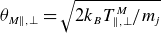 $\theta _{M \|, \perp } = \sqrt {2k_B T^M_{\|, \perp }/m_{\!j}}$
with the Maxwellian temperature
 $ T^M_{\|, \perp }$
, the Boltzmann constant
 $k_B$
, the particle rest mass
 $m_{\!j}$
of species
 $j$
and the normalisation constant reads
 $N_{\!M}=1/(\pi ^{3/2} \theta _{M,\|} \theta _{M, \perp }^2 )$
.
In situ observations in space plasmas also reveal suprathermal particle populations which manifest as high-energy tails of the observed distributions, that cannot be captured by Maxwellian models alone. These suprathermal tails are often described using
 $\kappa$
-distributions, originally introduced by Olbert (Reference Olbert1968) and widely applied in studying kinetic instabilities (Meneses, Gaelzer & Ziebell Reference Meneses, Gaelzer and Ziebell2018; Shaaban et al. Reference Shaaban, Lazar, López, Yoon and Poedts2021; López et al. Reference López, Shaaban and Lazar2021a
). The standard bi-
 $\kappa$
-distribution (SKD) can be written as (Lazar, Fichtner & Yoon Reference Lazar, Fichtner and Yoon2016)
 \begin{align} f_{\mathrm{SKD}}\left (v_{\|}, v_{\perp }, \kappa \right )=N_{\mathrm{SKD}}\left (1+\frac {v_{\|}^2}{\kappa \theta _{\|}^2}+\frac {v_{\perp }^2}{\kappa \theta _{\perp }^2}\right )^{-\kappa -1}, \end{align}
with normalisation
 \begin{align} N_{\mathrm{SKD}}=\frac {1}{\pi ^{3 / 2} \theta _{\|} \theta _{\perp }^2} \frac {\varGamma (\kappa +1)}{\kappa ^{3 / 2} \varGamma (\kappa -1 / 2)} , \end{align}
where
 $\varGamma$
denotes the gamma function. The parameter
 $\kappa$
controls the strength of the suprathermal tail and the distribution approaches a Maxwellian in the limit
 $\kappa \rightarrow \infty$
. The thermal speeds are
 $\theta _{ \|, \perp } = \sqrt {2k_B T^{\kappa }_{\|, \perp }/m}$
, with
 $T^{\kappa }_{\|, \perp }= ({\kappa }/({\kappa -3/2})) T^{M}_{\|, \perp } \gt T^{M}_{\|, \perp }$
and
 $\kappa \gt 3/2$
. A well-known limitation of the SKD is that higher-order velocity moments (including essential macro-parameters such as temperature, heat flux and transport coefficients) diverge (Scherer, Fichtner & Lazar Reference Scherer, Fichtner and Lazar2017), whereas the observed distributions may exhibit stronger tails corresponding to lower values of
 $\kappa$
(Štverák et al. Reference Štverák, Trávníček, Maksimovic, Marsch, Fazakerley and Scime2008; Gloeckler et al. Reference Gloeckler, Fisk, Mason, Roelof and Stone2012; Wilson et al. Reference Wilson III2019a
,
Reference Wilson IIIb
).
To overcome these shortcomings, the regularised
 $\kappa$
-distribution (RKD) has been introduced (Scherer et al. Reference Scherer, Fichtner and Lazar2017, see also Lazar & Fichtner (Reference Lazar and Fichtner2021)), modifying the SKD by introducing an exponential cutoff that guarantees the convergence of all velocity moments.
 \begin{align} \begin{aligned} f_{\mathrm{RKD}}\left (v_{\|}, v_{\perp }, \kappa , \alpha \right )= N_{\mathrm{RKD}}\!\left (1+\frac {v_{\|}^2}{\kappa \varTheta _{\|}^2}+\frac {v_{\perp }^2}{\kappa \varTheta _{\perp }^2}\right )^{-\kappa -1} \exp \!\left (-\frac {\alpha ^2 v_{\|}^2}{\varTheta _{\|}^2}-\frac {\alpha ^2 v_{\perp }^2}{\varTheta _{\perp }^2}\right ). \end{aligned} \end{align}
In this case the normalisation constant is (Scherer et al. Reference Scherer, Lazar, Husidic and Fichtner2019)
 \begin{align} N_{\mathrm{RKD}}=\frac {1}{\pi ^{3 / 2} \varTheta _{\|} \varTheta _{\perp }^2 W}, \end{align}
with
 \begin{align} W = U\!\left (\frac {3}{2}, \frac {3-2\kappa }{2},\alpha ^2 \kappa \right ), \end{align}
where
 $U$
denotes the Tricomi function (Oldham, Myland & Spanier Reference Oldham, Myland and Spanier2009). The parameter
 $\alpha \gt 0$
controls the exponential cutoff and is independent of
 $\kappa$
. The ‘thermal’ speeds are defined as
 $\varTheta _{\|, \perp }$
and differ from those defined in the SKD case. The RKD retains the desirable suprathermal behaviour of
 $\kappa$
distributions while ensuring that all velocity moments remain finite. Consequently, macroscopic plasma quantities are always consistently defined through velocity moments. The SKD and Maxwellian distributions are recovered as limiting cases for
 $\alpha \rightarrow 0$
and
 $\kappa \rightarrow \infty$
, respectively, see Scherer et al. (Reference Scherer, Fichtner and Lazar2017); Schröder et al. (Reference Schröder, Fichtner, Lazar, Verscharen and Klein2025a
). Applications of the RKD include the macroscopic description of suprathermal populations, modelling of anisotropic distributions measured in situ in the solar wind and the evaluation of transport properties in non-equilibrium plasmas (Lazar et al. Reference Lazar, Scherer, Fichtner and Pierrard2020; Scherer et al. Reference Scherer, Husidic, Lazar and Fichtner2021; Husidic et al. Reference Husidic, Scherer, Lazar, Fichtner and Poedts2022; Hau, Chang & Lazar Reference Hau, Chang and Lazar2023). A more detailed discussion of the RKD and its properties and applications can be found in Schröder et al. (Reference Schröder, Fichtner, Lazar, Verscharen and Klein2025a
,
Reference Schröder, Lazar, López and Fichtnerb
).
In the present study we extend the investigation of RKD plasmas within linear wave theory by considering arbitrary propagation angles with respect to the magnetic field. Earlier studies were largely restricted to parallel electromagnetic modes (Husidic et al. Reference Husidic, Lazar, Fichtner, Scherer and Astfalk2020; Schröder et al. Reference Schröder, Fichtner, Lazar, Verscharen and Klein2025a , Reference Schröder, Lazar, López and Fichtnerb ). Here, we include oblique propagation and focus on the electron and proton firehose instabilities (EFHI and PFHI, respectively).
Parallel firehose modes are oscillatory or periodic with finite real frequency (
 $\omega _r\neq 0$
), whereas oblique propagation also allows for purely non-propagating, aperiodic modes (
 $\omega _r=0$
). Linear theory predicts that the fastest-growing electron firehose modes occur at oblique angles and are typically aperiodic (Yoon, Wu & de Assis Reference Yoon, Wu and de Assis1993; Li & Habbal Reference Li and Habbal2000; Shaaban et al. Reference Shaaban, Lazar, López, Fichtner and Poedts2019). Hybrid simulations support these predictions (Gary & Nishimura Reference Gary and Nishimura2003; López et al. Reference López, Lazar, Shaaban, Poedts, Yoon, Viñas and Moya2019). For protons, aperiodic firehose modes can likewise dominate near instability thresholds when mixing with anisotropic electrons (López et al. Reference López, Micera, Lazar, Poedts, Lapenta, Zhukov, Boella and Shaaban2022), which is consistent with solar wind observations (Kasper et al. Reference Kasper, Lazarus and Gary2002; Bale et al. Reference Bale, Kasper, Howes, Quataert, Salem and Sundkvist2009). With isotropic electrons, periodic proton firehose modes are expected to dominate (Hellinger & Matsumoto Reference Hellinger and Matsumoto2000).
While dispersion relations for SKD plasmas can be solved analytically or numerically, e.g. via the DIS-K solver (López et al. Reference López, Shaaban and Lazar2021; López et al. Reference López, Shaaban and Lazar2021b ), a full (semi-)analytical solvable dispersion tensor and plasma dispersion functions for anisotropic RKD plasmas for oblique propagation have not yet been derived. However, such systems can be investigated numerically using the Arbitrary Linear Plasma Solver (ALPS) (Verscharen et al. Reference Verscharen, Klein, Chandran, Stevens, Salem and Bale2018). This solver determines, for arbitrary propagation angles, the linear Vlasov–Maxwell dispersion relation directly from tabulated background distribution functions and does not require explicit further analytical expressions.
1.2. Linear dispersion theory
First, we assume that the plasma fluctuations, specifically those of the electric and magnetic fields (
 $\boldsymbol{E}$
and
 $\boldsymbol{B}$
, respectively), are small enough to justify the application of linear theory. In order to investigate plasma instabilities, we solve the kinetic dispersion relation to obtain the complex frequency
 \begin{align} \omega (\boldsymbol{k}) = \omega _r(\boldsymbol{k}) + i\gamma (\boldsymbol{k}), \end{align}
where
 $\boldsymbol{k}$
is the wave vector corresponding to plane-wave-like fluctuations, and
 $\omega _r$
denotes the real and
 $\gamma$
the imaginary part of the frequency.
To obtain this solution, we use the linearised Vlasov equation and the linearised set of Maxwell’s equations, providing an expression for the plasma susceptibilities
 $\boldsymbol{\chi}_{\!j}$
for the
 $j$
th species (see Appendix A). These susceptibilities are then related to the plasma’s dielectric tensor
 $\boldsymbol{\epsilon }$
through
 \begin{align} \boldsymbol{\epsilon } = \unicode {x1D7D9} + \sum _j \boldsymbol{\chi}_{\!j}. \end{align}
From that, we can obtain the wave equation
 \begin{align} (\boldsymbol{k}c/\omega ) \times [(\boldsymbol{k}c/\omega ) \times \boldsymbol{E}] + \boldsymbol{\varepsilon } \boldsymbol{\cdot }\boldsymbol{E} \equiv \mathcal{D} \boldsymbol{\cdot }\boldsymbol{E} = 0 ,\end{align}
where
 $c$
is the speed of light. Solving
 $\text{det}\ \mathcal{D} = 0$
with
 $\boldsymbol{E}\neq 0$
provides non-trivial solutions. To obtain the latter, the ALPS code (Verscharen et al. Reference Verscharen, Klein, Chandran, Stevens, Salem and Bale2018) will be used, which offers a robust numerical approach, providing solutions for arbitrary linear plasma set-ups. ALPS has proven (and further proven with this study) to be a valuable tool for studying a wide range of plasma instabilities. For further details on its implementation and capabilities, refer to Verscharen et al. (Reference Verscharen, Klein, Chandran, Stevens, Salem and Bale2018) and Klein & Verscharen (Reference Klein and Verscharen2025).
The structure of the paper is as follows. We begin with a brief description of our set-up in § 2. In the first part of this section, the ALPS implementation is validated against a series of previous results, in particular, those obtained for oblique EFHI modes in Maxwellian plasmas (Li & Habbal Reference Li and Habbal2000; Maneva et al. Reference Maneva, Lazar, Viñas and Poedts2016), SKD plasmas (Shaaban et al. Reference Shaaban, Lazar, López, Fichtner and Poedts2019) and for oblique PFHI in Maxwellian plasmas (Hellinger & Matsumoto Reference Hellinger and Matsumoto2000; Maneva et al. Reference Maneva, Lazar, Viñas and Poedts2016). The new RKD results are presented and discussed in the third section. All findings are summarised in the concluding § 4.
2. Model set-up and validation results
We focus on the oblique electron and proton firehose instabilities (OEFHI, OPFHI) in a two-component plasma comprising protons (
 $p$
) and electrons (
 $e$
) with one population each. The plasma frequency of species
 $j$
is defined as
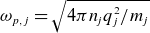 $\omega _{p,j} = \sqrt {4 \pi n_{\!j} q_j^2 / m_{\!j}}$
, and the corresponding non-relativistic gyrofrequency as
 $\varOmega _j = q_j B_0 / (m_{\!j} c)$
, where
 $q_j$
and
 $n_{\!j}$
denote the electric charge and number density of species
 $j$
, protons (
 $j = p$
) and electrons (
 $j = e$
), respectively. The parallel plasma beta of each species
 $j$
is
 $\beta _j = 8 \pi n_{\!j} k_B T_{j, \parallel } /B_0^2$
, with the magnitude of the background magnetic field
 $B_0$
and the normalised number density set to
 $n_e/n_0=n_p/n_0=1.0$
. The temperature anisotropy may be defined as
 $A_j=T_{j, \perp }/T_{j,\|}$
. We use a proton-to-electron mass ratio of
 $m_p/m_e = 1836$
and assume the electron plasma-to-gyrofrequency ratio to be
 $\omega _{p,e}/|\varOmega _e|=1000$
. By allowing for arbitrary propagation directions, we extend the study by Husidic et al. (Reference Husidic, Lazar, Fichtner, Scherer and Astfalk2020), which was limited to electromagnetic modes parallel to the magnetic field, and by Shaaban et al. (Reference Shaaban, Lazar, López, Fichtner and Poedts2019), which was limited to oblique modes of SKDs. The present investigation explores the effects of RKD distributed plasmas with an isotropic cutoff,
 $\alpha _{\perp }=\alpha _{\|}\equiv \alpha$
on the dispersion relation for oblique propagation, comparing them with the results obtained for Maxwellian distributions and SKDs. Aperiodic branches with vanishing real frequency are observed in the oblique cases.
Normalised wave frequencies (left) and normalised growth rates (right) as functions of the normalised wavenumber for OEFHI at different propagation angles (
 $0^\circ$
,
 $17^\circ$
,
 $20^\circ$
,
 $22^\circ$
and
 $24^\circ$
, from top to bottom), obtained with ALPS (solid lines) and DIS-K (dots) for the Maxwellian case.

Figure 1. Long description
The image contains ten line graphs arranged in two columns and five rows. Each row corresponds to a different propagation angle (θ = 0°, 17°, 20°, 22°, and 24°). The left column shows normalized wave frequencies (ω/Ωp) as a function of the normalized wavenumber (kc/ωp,p). The right column shows normalized growth rates (γ/Ωp) as a function of the normalized wavenumber (kc/ωp,p). Each graph compares results obtained with ALPS (solid lines) and DIS-K (dots) for the Maxwellian case. The x-axis for all graphs is labeled ‘kc/ωp,p’ and the y-axis is labeled ‘ω/Ωp’ for the left column and ‘γ/Ωp’ for the right column. The graphs illustrate how wave frequencies and growth rates vary with the wavenumber for different propagation angles.
2.1. Validation. The OEFHI with Maxwellian and SKD
To begin with, the ALPS set-up is validated against previous results for EFHI driven by bi-Maxwellian electrons (Li & Habbal Reference Li and Habbal2000), which here are reproduced using DIS-K, imposing the same plasma parameters. For the electrons,
 $\beta _{e}=5$
and
 $T_{e,\perp }/T_{e,\parallel }=0.5$
, while the protons are described by an isotropic Maxwellian with
 $\beta _{p}=1$
. Figure 1 presents the (O)EFHI dispersion curves for different propagation angles (
 $0^\circ$
,
 $17^\circ$
,
 $20^\circ$
,
 $22^\circ$
and
 $24^\circ$
, from top to bottom), obtained with ALPS (solid lines) and DIS-K (dots). Both the wave frequency (left) and growth rate (right) are shown as functions of the wavenumber
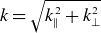 $k=\sqrt {k^2_{\|} + k^2_{\perp }}$
. Overall, the agreement between the two solvers is very good across all propagation angles (less than
 $0.2\,\%$
deviation for the maximum growth rate
 $\gamma _m$
and the corresponding wavenumber
 $k_m$
). Note that these results were also replicated by NHDS (Verscharen & Chandran (Reference Verscharen and Chandran2018)) and PLUME (Klein, Howes & Brown (Reference Klein, Howes and Brown2025)), agreeing with DIS-K and ALPS.
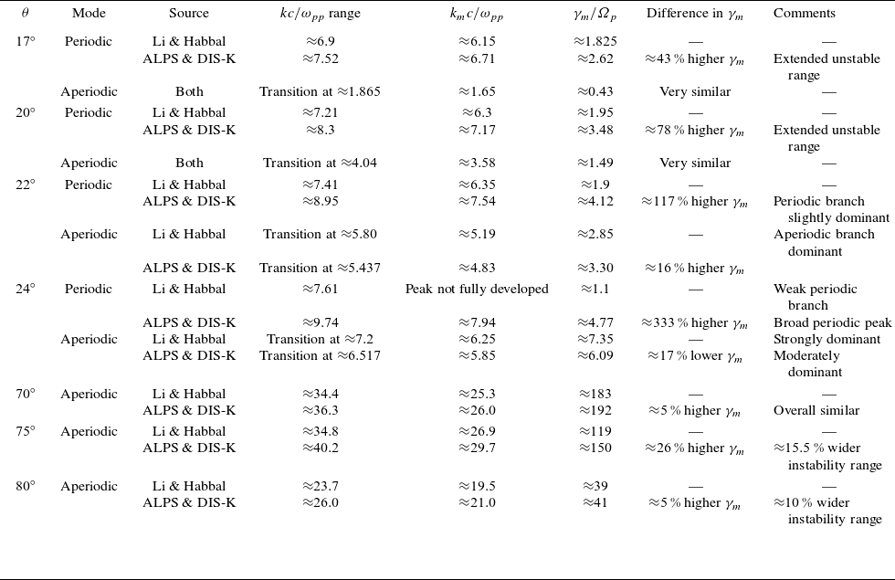
For parallel propagation, the agreement between figure 1(a) in Li & Habbal (Reference Li and Habbal2000) and our results is excellent. However, for oblique propagation, noticeable differences arise, as evidenced by a comparison of the unstable solutions in our figure 1 and figure 1 in Li & Habbal (Reference Li and Habbal2000). The present results can be regarded as an updated version, and a detailed comparison between the results reported by Li & Habbal (Reference Li and Habbal2000) and the present ALPS/DIS-K solutions is summarised in table 1. For the periodic branch, the largest deviations are found at finite propagation angles, where the present solutions exhibit systematically higher growth rates and larger ranges of unstable wavenumbers. Differences in the aperiodic branch are generally smaller, although with some noticeable deviations in the transition region between periodic and aperiodic modes, see the results for
 $\theta = 22^\circ$
and
 $\theta = 24^\circ$
. At
 $\theta = 22^\circ$
, in the present ALPS/DIS-K solutions the periodic peak remains slightly dominant with
 $\gamma _m$
approximately
 $1.25$
times larger than the aperiodic peak, in contrast to the dominant aperiodic branch (with
 $\gamma _m$
approximately
 $1.5$
times larger than the periodic one) reported by Li & Habbal (Reference Li and Habbal2000).
More significant differences are found at
 $\theta = 24^\circ$
. While Li & Habbal (Reference Li and Habbal2000) show a strongly dominant aperiodic branch with
 $\gamma _m$
approximately
 $6.7$
times larger than the periodic branch with a non-developed peak, the present solutions instead exhibit two distinguishable peaks, with only a moderate dominance of the aperiodic one (approximately
 $1.27$
times larger than the periodic peak). In addition, the periodic branch obtained here remains unstable over a wider wavenumber interval with a markedly higher and broader peak.
Normalised growth rates as functions of the normalised wavenumber for aperiodic OEFHI at different propagation angles (
 $30^\circ$
,
 $40^\circ$
,
 $50^\circ$
,
 $60^\circ$
,
 $70^\circ$
,
 $75^\circ$
and
 $80^\circ$
), obtained with ALPS (solid lines) and DIS-K (dots) for the Maxwellian case.
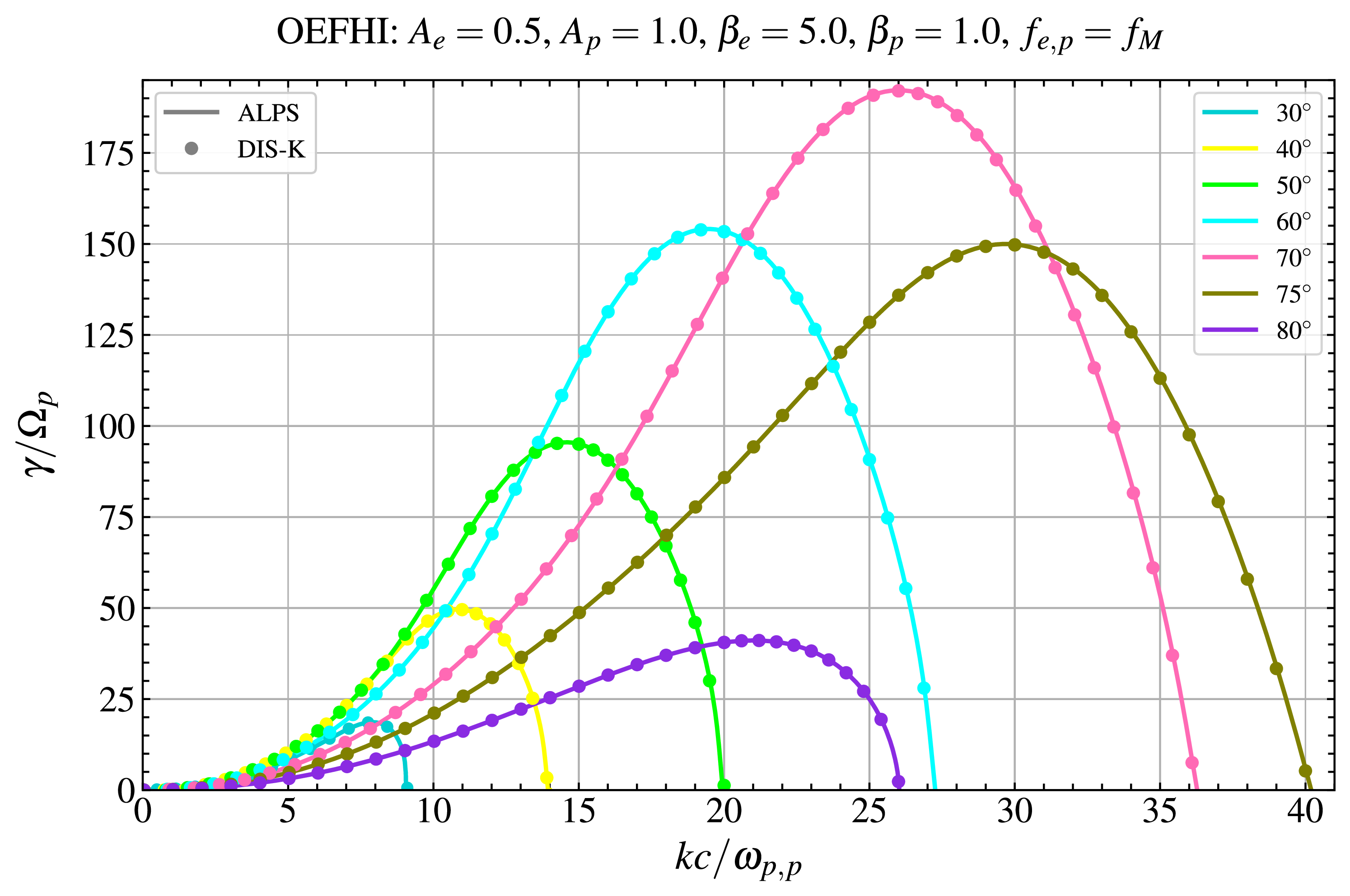
Figure 2 shows the growth rates of aperiodic modes at higher propagation angles, with ALPS results indicated by solid lines and DIS-K with dots. The agreement between both solvers remains very good in all cases (less than
 $0.1\,\%$
deviation in terms of
 $\gamma _m$
and
 $k_m$
). The overall solutions are in good qualitative agreement with the results in Li & Habbal (Reference Li and Habbal2000) (see their figure 3), including the shift of the growth rates toward higher wavenumbers and an increase of
 $\gamma _m$
up to
 $\theta =70^\circ$
, followed by a decrease at larger angles. However, we find notable quantitative differences, which are summarised in table 1.
The present solutions systematically predict broader unstable wavenumber intervals and, in most cases, enhanced maximum growth rates compared with Li & Habbal (Reference Li and Habbal2000). Despite the qualitative agreement, differences are quantitatively noticeable for the periodic branch at finite angles, and for the extent of the unstable range and the maximum growth rates of high-angle aperiodic solutions.
Normalised growth rates as functions of the normalised wavenumber, for the oblique (aperiodic) EFHI at propagation angles
 $60^\circ$
,
 $70^\circ$
,
 $75^\circ$
and
 $80^\circ$
for SKD with
 $\kappa =3.0$
, obtained with ALPS (solid lines) and DIS-K (dots).
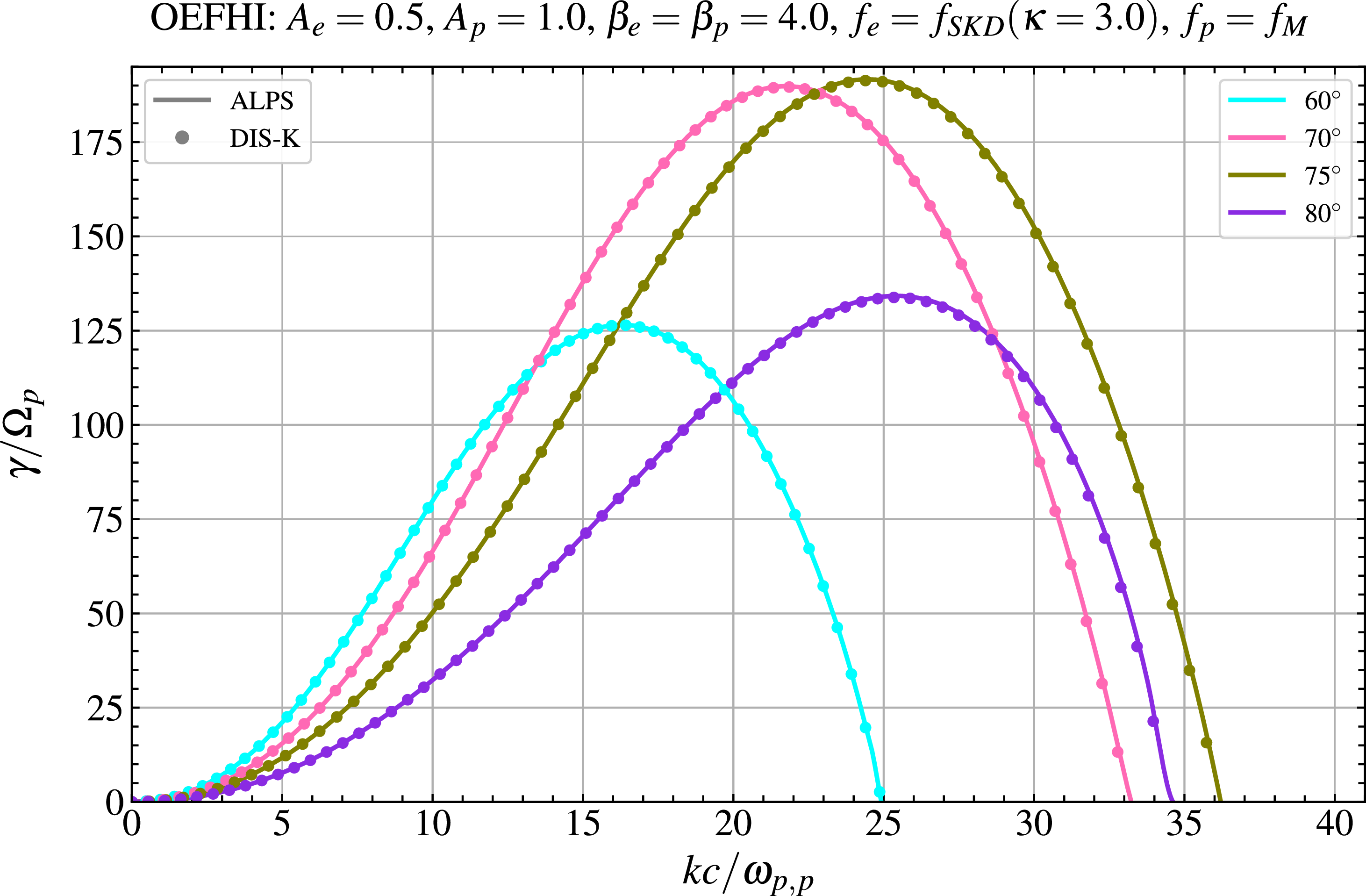
Now we validate ALPS with OEFHI solutions obtained for SKD electrons with DIS-K; see also previous results in Shaaban et al. (Reference Shaaban, Lazar, López, Fichtner and Poedts2019). Thus, figure 3 shows the comparison of the normalised growth rate between ALPS and DIS-K for the aperiodic OEFHI for different angles (
 $60^\circ$
,
 $70^\circ$
,
 $75^\circ$
and
 $80^\circ$
) for SKD electrons with
 $\kappa = 3.0$
. The agreement between both solvers is very good for all cases (less than
 $0.4\,\%$
deviation in terms of
 $\gamma _m$
and
 $k_m$
). For bi-Maxwellian electrons, Li & Habbal (Reference Li and Habbal2000) imposed an electron–proton temperature ratio of
 $T_{e,\|}/T_{p, \|} = 5$
. To minimise the effect of the cyclotron resonant protons for the
 $\kappa$
-distributed plasma cases, we use
 $\beta _e = \beta _p = 4.0$
for the further study of the OEFHI.
In figure 4, contour plots, derived with DIS-K, of the OEFHI normalised frequency (left panel) and growth rate (right panel), in the
 $k$
–
 $\theta$
-plane are shown for the Maxwellian case (top) and for the SKD with
 $\kappa =3.0$
(bottom). While the Maxwellian case has unstable periodic solutions up to
 $\theta \approx 18^\circ$
and
 $kc/\omega _{pp} \approx 8.1$
, the SKD case has unstable periodic solutions up to an increased
 $\theta \approx 31^\circ$
and decreased
 $kc/\omega _{pp} \approx 4.1$
. The aperiodic mode is unstable for the Maxwellian case up to
 $\theta \approx 73^\circ$
and
 $kc/\omega _{pp} \approx 37$
. The maximum growth rate is reached at
 $\theta _m \approx 65.1^\circ$
with
 $\gamma _m \approx 122.5$
at
 $k_m c/\omega _{pp}\approx 24.1$
. For the SKD case, the aperiodic mode is unstable until
 $\theta \approx 89^\circ$
and
 $kc/\omega _{pp} \approx 36.5$
. The maximum growth rate is reached at
 $\theta _m \approx 72.9^\circ$
with
 $\gamma _m \approx 195.6$
at
 $k_m c/\omega _{pp}\approx 23.2$
.
The validation for the OPFHI, inspired by Hellinger & Matsumoto (Reference Hellinger and Matsumoto2000), can be found in Appendix C, showing again very good agreement. These applications to the OEFHI and OPFHI validate both the ALPS and the DIS-K code as reliable tools, because the same results were obtained with rather different numerical algorithms. We note that ALPS is computationally more demanding than DIS-K (or general (semi-)analytic solvers), since it evaluates the dispersion relation through more complex numerical integration schemes over tabulated distribution functions, whereas DIS-K relies on analytical expressions for the SKD plasma dispersion functions. In addition, the findings for the modes in an SKD plasma can now serve as a reference for the RKD ones discussed in the following.
Contour plot of the OEFHI normalised frequency (left panel) and growth rate (right panel) in the
 $k$
–
 $\theta$
-plane for the Maxwellian case (top) and SKD case with
 $\kappa =3.0$
(bottom), obtained with DIS-K.
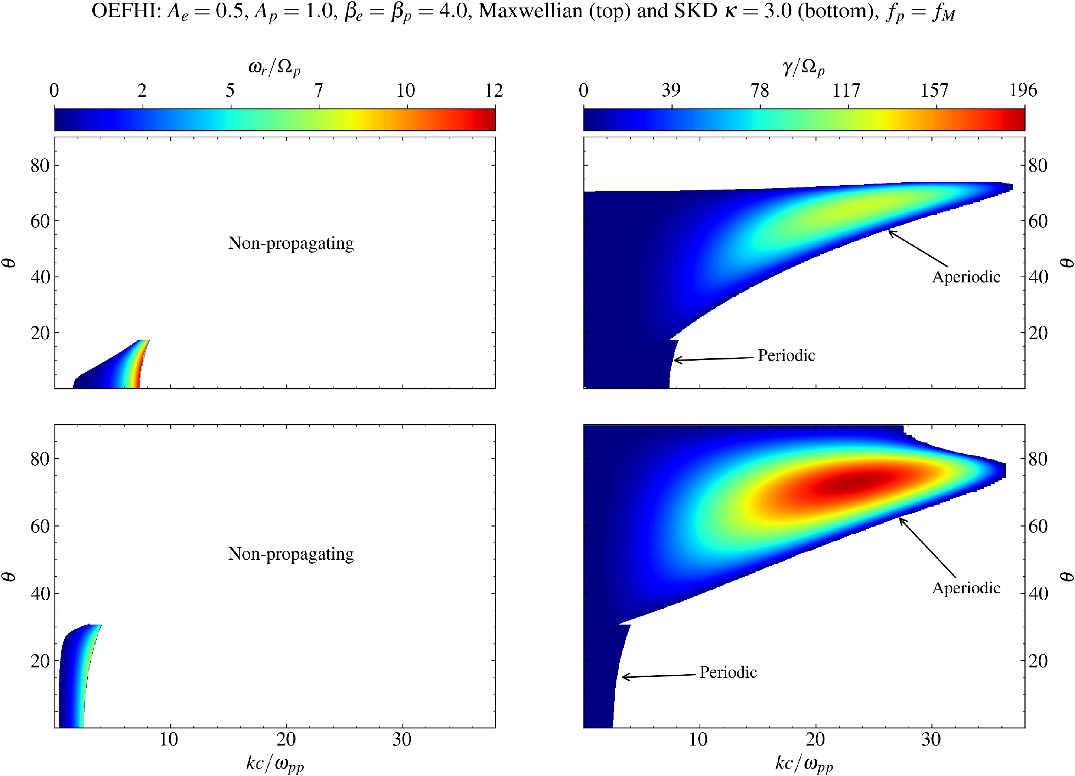
Figure 4. Long description
The image contains four contour plots. Panel A and Panel B show the Maxwellian case, while Panel C and Panel D show the SKD case with kappa equal to 3.0. Each panel is divided into two subplots: the left subplot displays the normalized frequency, and the right subplot displays the growth rate. The x-axis in all subplots is labeled ‘kc/ωpp’ and ranges from 0 to 35. The y-axis is labeled ‘θ’ and ranges from 0 to 80 degrees. The color scale at the top of each subplot indicates the values of the normalized frequency and growth rate, with blue representing lower values and red representing higher values. In the Maxwellian case, the left subplot shows a non-propagating region, while the right subplot distinguishes between periodic and aperiodic regions. Similarly, the SKD case with kappa equal to 3.0 shows non-propagating regions in the left subplot and periodic and aperiodic regions in the right subplot.
3. New results: oblique firehose modes for RKDs
Imposing plasma parameters identical to those adopted for the validation of the OEFHI and OPFHI cases, the analysis is extended here to RKD plasmas, using ALPS.
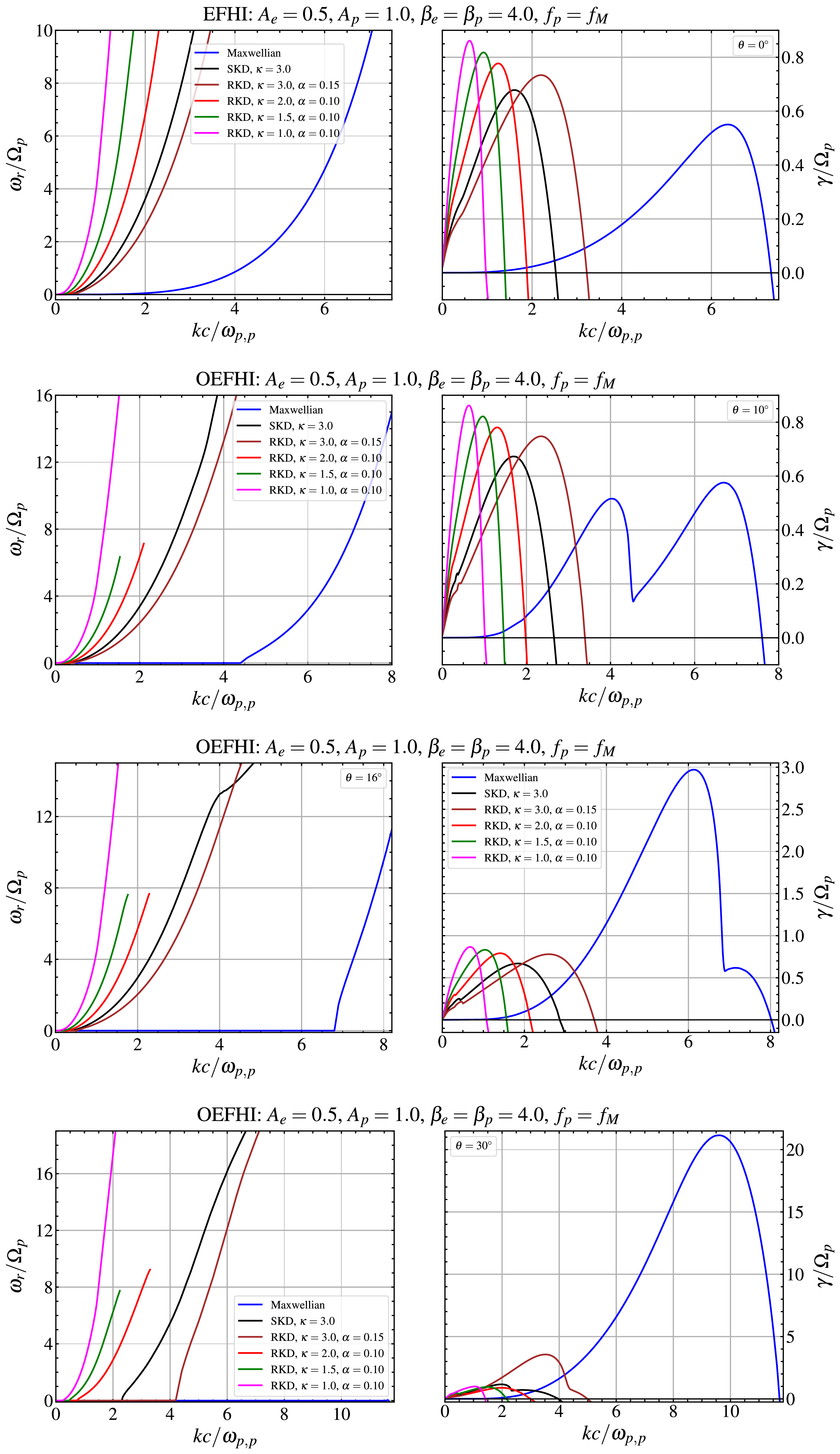
Normalised wave frequencies (left) and normalised growth rates (right) as functions of the normalised wavenumber for OEFHI at different propagation angles (
 $0^\circ$
,
 $10^\circ$
,
 $16^\circ$
and
 $30^\circ$
, from top to bottom), obtained with ALPS for for Maxwellian, SKD and different RKDs.
Normalised wave frequencies (left) and normalised growth rates (right) as functions of the normalised wavenumber for OEFHI at different propagation angles (
 $16^\circ$
and
 $30^\circ$
, from top to bottom, same as in figure 5, but with more compact plotting scales), obtained with ALPS for Maxwellian, SKD and different RKDs.

Figure 6. Long description
The image contains four line graphs. Panel A and Panel B show data for a propagation angle of 16 degrees, while Panel C and Panel D show data for a propagation angle of 30 degrees. Each graph plots normalized wave frequencies or growth rates against normalized wavenumber. The x-axis for all graphs is labeled ‘kc / ωp,p’ and the y-axes are labeled ‘ωr / Ωp’ for the left graphs and ‘γ / Ωp’ for the right graphs. Different lines represent Maxwellian, SKD, and various RKD models, each with distinct colors: blue for Maxwellian, black for SKD, red for RKD with κ = 3.0 and α = 0.15, green for RKD with κ = 2.0 and α = 0.10, and magenta for RKD with κ = 1.0 and α = 0.10. The graphs illustrate how these models vary in their predictions of wave frequencies and growth rates across different wavenumbers and propagation angles.
3.1. Oblique electron firehose instability
Figure 5 shows for the (O)EFHI normalised frequencies in the left panels and normalised growth rates in the right panels for different propagation angles (
 $0^\circ$
,
 $10^\circ$
,
 $16^\circ$
and
 $30^\circ$
, from top to bottom) and for several VD functions: Maxwellian (blue), SKD with
 $\kappa =3.0$
(black), RKD with
 $\kappa =3.0$
and
 $\alpha =0.15$
(brown), RKD with
 $\kappa =2.0$
and
 $\alpha =0.10$
(red), RKD with
 $\kappa =1.5$
and
 $\alpha =0.1$
(green) and RKD with
 $\kappa =1.0$
and
 $\alpha =0.10$
(magenta). Figure 6 shows the same results for
 $16^\circ$
and
 $30^\circ$
, but with more compact plotting scales for better visibility of the SKD and RKD solutions. Because all RKDs have different
 $\kappa$
values, they will be distinguished only by their
 $\kappa$
values throughout this analysis, for convenience.
The parallel EFHI case, where only periodic modes are present, has been discussed by Schröder et al. (Reference Schröder, Fichtner, Lazar, Verscharen and Klein2025a
). The present results are consistent with those findings and can be summarised as follows. Compared with the Maxwellian case, the use of an SKD with
 $\kappa =3.0$
leads to an increase in the maximum growth rate and a shift toward lower wavenumbers, accompanied by a reduction of the unstable wavenumber range. The real frequency exhibits a similar shift toward lower wavenumbers, with enhanced values. Using an RKD with the same
 $\kappa =3.0$
value and
 $\alpha =0.15$
, thus reducing the suprathermal tails of the VD, shifts both the real and imaginary solutions towards the Maxwellian solution. The maximum growth rate is slightly enhanced, since the moderate cutoff increases the effective anisotropy. Using RKDs with lower
 $\kappa$
values and a moderate cutoff (
 $\alpha =0.1$
) maintains the pattern observed for the SKD. As
 $\kappa$
decreases (while keeping
 $\alpha$
constant), corresponding to an enhanced population of suprathermal particles, the maximum growth rate increases further and shifts to lower wavenumbers, resulting in a more pronounced and narrower peak. For example, while the Maxwellian case yields
 $\gamma _m/\varOmega _p = 0.55$
at
 $k_m c/\omega _{pp} = 6.36$
, the RKD case with
 $\kappa =1.0$
gives
 $\gamma _m/\varOmega _p = 0.86$
at
 $k_m c/\omega _{pp} = 0.61$
, corresponding to an increase by a factor of
 $1.56$
and a reduction in
 $k_m$
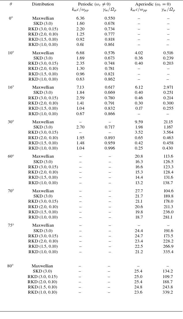
by approximately one order of magnitude. Further values regarding the maximum growth rates for the different (O)EFHI cases can be found in table 2.
At
 $\theta = 10^\circ$
, the Maxwellian case exhibits a distinct aperiodic peak with
 $\gamma _m/\varOmega _p = 0.516$
at
 $k_m c/\omega _{pp} = 4.024$
, which competes with a periodic branch that remains dominant (we refer to a mode as dominant if its maximum growth rate is higher than the maximum growth rates of all other solutions to the linear dispersion relation), with approximately
 $11.6\,\%$
higher
 $\gamma _m/\varOmega _p = 0.576$
at
 $k_m c/\omega _{pp} = 6.68$
. Compared with the parallel case, the periodic peak shows a very similar maximum growth rate (increase of less than
 $5\,\%$
), with a slight shift toward higher
 $k_m$
. For the SKD case, a marginal aperiodic peak appears at low wavenumbers, with
 $\gamma _m/\varOmega _p = 0.239$
at
 $k_m c/\omega _{pp} = 0.363$
. The periodic branch clearly dominates, reaching a significantly higher
 $\gamma _m$
, approximately
 $182\,\%$
larger than the aperiodic peak. Relative to the parallel case, the propagating mode remains nearly unchanged in
 $\gamma _m$
, with only a minor shift toward higher
 $k_m$
. The same behaviour is seen for the RKD with
 $\kappa = 3.0$
. The aperiodic peak is slightly more pronounced, but is lower in terms of
 $\gamma _m$
(
 $\gamma _m/\varOmega _p = 0.203$
at
 $k_m c/\omega _{pp} = 0.408$
) compared with the SKD cases. All three RKD cases with lower
 $\kappa$
-values exhibit only a periodic peak. In comparison with the parallel case, this peak is essentially unchanged in terms of
 $\gamma _m$
(increase of below
 $0.5\,\%$
), with only a slight shift toward higher
 $k_m$
(
 ${\lesssim}4\,\%$
). Notably, the periodic peaks of all SKD and RKD cases exceed both the periodic and aperiodic peaks of the Maxwellian case. At certain values of
 $k$
, where
 $\gamma \lt 0$
, the solutions corresponding to the unstable branch jump to a different branch for the RKDs with
 $\kappa = 2.0$
and
 $\kappa = 1.5$
. This behaviour is not shown here (nor at other angles), as it is not the focus of the present analysis.
At
 $\theta = 16^\circ$
, the Maxwellian case is clearly dominated by the aperiodic branch, with
 $\gamma _m/\varOmega _p = 2.971$
, approximately
 $382\,\%$
higher than the periodic peak (
 $\gamma _m/\varOmega _p = 0.617$
). The latter shows only a slight increase compared with the parallel case and
 $\theta = 10^\circ$
. However, as the aperiodic branch extends to higher wavenumbers, the periodic branch becomes effectively truncated. For the SKD case, the aperiodic mode becomes more pronounced and slightly enhanced compared with
 $\theta = 10^\circ$
, reaching
 $\gamma _m/\varOmega _p = 0.251$
at
 $k_m c/\omega _{pp} = 0.408$
. Nevertheless, it remains significantly weaker than the periodic mode, which attains
 $\gamma _m/\varOmega _p = 0.669$
at
 $k_m c/\omega _{pp} = 1.844$
. As in the previous cases, the periodic branch shows only a modest increase in
 $\gamma _m$
and a slight shift toward higher
 $k_m$
. The RKD with
 $\kappa =3.0$
shows the same development with respect to the periodic peak (
 $\gamma _m/\varOmega _p = 0.780$
at
 $k_m c/\omega _{pp} = 2.594$
) and aperiodic peak (
 $\gamma _m/\varOmega _p = 0.214$
at
 $k_m c/\omega _{pp} = 0.467$
.) The RKD with
 $\kappa =2.0$
develops a weak aperiodic mode at
 $k_m c/\omega _{pp} = 0.307$
with
 $\gamma _m/\varOmega _p = 0.300$
(approximately
 $19.5\,\%$
higher than in the SKD case), together with a dominant periodic mode reaching
 $\gamma _m/\varOmega _p = 0.781$
, approximately
 $160\,\%$
larger. The periodic branch remains very similar to the corresponding peaks at lower angles. The RKDs with
 $\kappa =1.5$
and
 $\kappa =1.0$
exhibit only a periodic mode, with values closely matching those obtained at smaller propagation angles. Although the periodic modes in the SKD and RKD cases exceed the corresponding periodic peak of the Maxwellian (by a similar factor as for lower angles), the Maxwellian aperiodic mode has the largest growth rate overall. In particular, it exceeds the periodic mode of the RKD with
 $\kappa =1.0$
by approximately
 $245\,\%$
, and is roughly an order of magnitude larger than the aperiodic mode of the RKD with
 $\kappa =2.0$
.
At
 $\theta = 30^\circ$
, the Maxwellian case exhibits only a non-propagating mode, with a strongly enhanced growth rate reaching
 $\gamma _m/\varOmega _p = 21.15$
at
 $k_m c/\omega _{pp} = 9.599$
, together with an extended range of unstable wavenumbers. In contrast to lower angles, the SKD case shows a dominant aperiodic mode, with
 $\gamma _m/\varOmega _p = 2.705$
at
 $k_m c/\omega _{pp} = 0.717$
, exceeding the periodic mode (
 $\gamma _m/\varOmega _p = 1.167$
at
 $k_m c/\omega _{pp} = 1.984$
) by approximately
 $63\,\%$
. Using an RKD with
 $\kappa =3.0$
, the periodic peak is barley developed, due to the competition with the aperiodic mode, which gets significantly enhanced (more than an order of a magnitude compared with
 $\theta =16^\circ$
), with
 $\gamma _m=3.564$
at
 $k_m c/\omega _{pp} = 3.520$
exceeding those of the other SKD/RKD cases (by roughly
 $670\,\%$
) and showing a clear trend towards the Maxwellian solutions due to the cutoff of the suprathermal tails. For the RKD with
 $\kappa =2.0$
, the non-propagating peak is enhanced, reaching
 $\gamma _m/\varOmega _p = 0.463$
, which is approximately
 $54\,\%$
higher than at
 $\theta = 16^\circ$
. Nevertheless, the propagating mode remains dominant, with
 $\gamma _m/\varOmega _p = 0.893$
, approximately
 $93\,\%$
larger. The RKD cases with lower
 $\kappa$
values (
 $\kappa =1.5$
and
 $\kappa =1.0$
) develop aperiodic modes at this angle, in contrast to the behaviour at lower
 $\theta$
. These aperiodic contributions become less pronounced as
 $\kappa$
decreases. The maximum growth rates, however, remain similar across the RKD cases, with
 $\gamma _m/\varOmega _p = 0.458$
for
 $\kappa =1.5$
and
 $\gamma _m/\varOmega _p = 0.430$
for
 $\kappa =1.0$
and approximately two times smaller than those of the corresponding periodic ones. The periodic peaks are slightly enhanced and shifted toward higher wavenumbers. For example, relative to the parallel case, the RKD
 $\kappa =1.0$
case shows an increase of approximately
 $16\,\%$
in
 $\gamma _m$
and
 $72\,\%$
in
 $k_m$
. Overall, the maximum growth rate in the Maxwellian case exceeds those of the SKD and RKD cases by more than an order of magnitude.
Normalised growth rates as functions of the normalised wavenumber, for the (aperiodic) OEFHI at propagation angles
 $60^\circ$
,
 $70^\circ$
,
 $75^\circ$
and
 $80^\circ$
for Maxwellian and different RKDs.
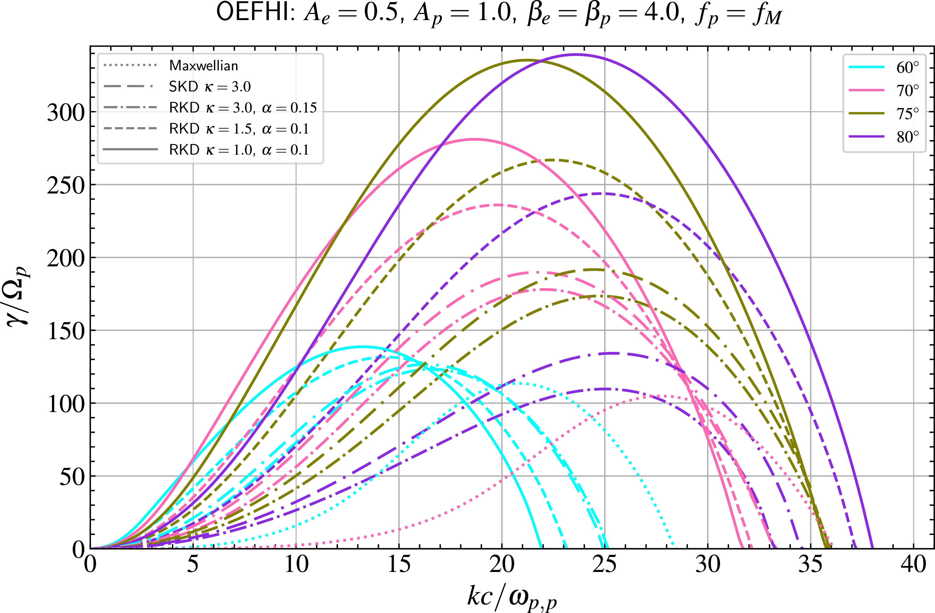
Figure 7 presents the normalised growth rates for higher propagation angles (
 $60^\circ$
,
 $70^\circ$
,
 $75^\circ$
and
 $80^\circ$
) for the Maxwellian case and for RKDs, obtained with ALPS. At these angles, only non-propagating modes are found, which are in general more than two orders of a magnitude higher then the periodic growth rates at parallel propagation. At
 $\theta = 60^\circ$
, the RKD cases exhibit higher growth rates than the Maxwellian case, in contrast to the behaviour at intermediate angles. As
 $\kappa$
decreases, the maximum growth rate increases and shifts toward lower wavenumbers. This trend is consistently observed for all angles considered here. The RKD with
 $\kappa =3.0$
shows always lower maximum growth rates (approximately
 $2\,\%$
–
 $18\,\%$
) and a shift towards the Maxwellian solution compared with the SKD case. At
 $\theta = 70^\circ$
, the Maxwellian case has already passed its maximum growth rate (see figure 4, where the maximum occurs at
 $\theta \approx 65^\circ$
) and begins to decrease. In contrast, all RKD cases show a significant amplification of the growth rate, accompanied by a shift toward higher wavenumbers. For example, the RKD case with
 $\kappa = 1.0$
reaches
 $\gamma _m/\varOmega _p = 282.1$
, corresponding to an increase of
 $103\,\%$
relative to
 $\theta = 60^\circ$
(
 $\gamma _m/\varOmega _p = 138.7$
), and an increase of
 $170\,\%$
compared with the Maxwellian value
 $\gamma _m/\varOmega _p = 104.6$
at
 $\theta = 70^\circ$
. The Maxwellian case, however, spans a broader range of unstable wavenumbers. The RKD with
 $\kappa =3.0$
reaches its maximum growth rate at
 $\theta = 70^\circ$
with
 $\gamma _m =178.0$
At
 $\theta = 75^\circ$
, both
 $\gamma _m$
and
 $k_m$
increase further for the RKD cases with lower
 $\kappa$
-values, leading to broad and pronounced peaks. The cases with
 $\kappa = 2.0$
and
 $\kappa = 1.5$
reach their maximum growth rates near this angle, with
 $\gamma _m/\varOmega _p = 228.2$
and
 $\gamma _m/\varOmega _p = 266.9$
, respectively. The Maxwellian case exhibits no unstable solutions at this angle (see figure 4, where instability is limited to
 $\theta \approx 73^\circ$
). At
 $\theta = 80^\circ$
, the maximum growth rates for
 $\kappa = 3.0$
and
 $\kappa = 1.5$
decrease and shift toward higher wavenumbers. In contrast, the case with
 $\kappa = 1.0$
attains its maximum near this angle, producing a broad peak that extends over a wide wavenumber interval (up to
 $kc/\omega _{pp} \approx 38$
), with
 $\gamma _m/\varOmega _p = 339.2$
at
 $k_m c/\omega _{pp} = 23.6$
, which is an increase of the growth rate of a factor of roughly 400 compared with the corresponding parallel propagation. These results would not be possible to achieve using SKDs for which the condition
 $\kappa \gt 1.5$
must be fulfilled.
Normalised wave frequencies (left) and normalised growth rates (right) as functions of the normalised wavenumber for OPFHI at different propagation angles (
 $0^\circ$
,
 $10^\circ$
,
 $35^\circ$
, from top to bottom), obtained with ALPS for Maxwellian, SKD and different RKDs.

Figure 8. Long description
Panel A: The top left graph is a line graph showing normalized wave frequencies as a function of normalized wavenumber for a propagation angle of 0 degrees. The x-axis is labeled ‘kc/ωp,p’ and the y-axis is labeled ‘ωr/Ωp’. Multiple lines represent different distributions: Maxwellian, SKD, and various RKDs. Panel B: The top right graph is a line graph showing normalized growth rates as a function of normalized wavenumber for a propagation angle of 0 degrees. The x-axis is labeled ‘kc/ωp,p’ and the y-axis is labeled ‘γ/Ωp’. Multiple lines represent different distributions: Maxwellian, SKD, and various RKDs. Panel C: The middle left graph is a line graph showing normalized wave frequencies as a function of normalized wavenumber for a propagation angle of 10 degrees. The x-axis is labeled ‘kc/ωp,p’ and the y-axis is labeled ‘ωr/Ωp’. Multiple lines represent different distributions: Maxwellian, SKD, and various RKDs. Panel D: The middle right graph is a line graph showing normalized growth rates as a function of normalized wavenumber for a propagation angle of 10 degrees. The x-axis is labeled ‘kc/ωp,p’ and the y-axis is labeled ‘γ/Ωp’. Multiple lines represent different distributions: Maxwellian, SKD, and various RKDs. Panel E: The bottom left graph is a line graph showing normalized wave frequencies as a function of normalized wavenumber for a propagation angle of 35 degrees. The x-axis is labeled ‘kc/ωp,p’ and the y-axis is labeled ‘ωr/Ωp’. Multiple lines represent different distributions: Maxwellian, SKD, and various RKDs. Panel F: The bottom right graph is a line graph showing normalized growth rates as a function of normalized wavenumber for a propagation angle of 35 degrees. The x-axis is labeled ‘kc/ωp,p’ and the y-axis is labeled ‘γ/Ωp’. Multiple lines represent different distributions: Maxwellian, SKD, and various RKDs.
3.2. Oblique proton firehose instability
Figure 8 shows the (O)PFHI dispersion relations (normalised frequencies in the left panels and normalised growth rates in the right panels) for different propagation angles (
 $0^\circ$
,
 $10^\circ$
and
 $35^\circ$
, from top to bottom) and for several VD functions: Maxwellian (blue), SKD with
 $\kappa =3.0$
(black), RKD with
 $\kappa =3.0$
and
 $\alpha =0.15$
(brown), RKD with
 $\kappa =2.0$
and
 $\alpha =0.1$
(red), RKD with
 $\kappa =1.5$
and
 $\alpha =0.1$
(green) and RKD with
 $\kappa =1.0$
and
 $\alpha =0.1$
(magenta).
For the parallel case, where only periodic modes are present, the results are in qualitative agreement with those reported by Husidic et al. (Reference Husidic, Lazar, Fichtner, Scherer and Astfalk2020). They can be summarised as follows. Using an SKD with low
 $\kappa$
enhances the growth rate and shifts
 $\gamma _m$
toward lower wavenumbers compared with the Maxwellian case. The real frequency is also enhanced at low to intermediate wavenumbers. This trend persists when employing RKDs with lower
 $\kappa$
(at fixed, moderate
 $\alpha$
), corresponding to an increased population of suprathermal particles in the tails. For example, the Maxwellian case yields
 $\gamma _m/\varOmega _p = 0.123$
at
 $k_m c/\omega _{pp} = 0.279$
, whereas the RKD with
 $\kappa = 1.0$
gives
 $\gamma _m/\varOmega _p = 0.169$
at
 $k_m c/\omega _{pp} = 0.131$
, corresponding to an increase of approximately
 $37\,\%$
in
 $\gamma _m$
and a reduction of approximately
 $113\,\%$
in
 $k_m$
. Using an RKD with
 $\kappa =3.0$
, the overall growth rate gets slightly reduced (approximately
 $2\,\%$
in terms of
 $\gamma _m$
) and shifted towards the Maxwellian case. The range of unstable wavenumbers remains approximately the same for all VDs.
At
 $\theta = 10^\circ$
, only propagating modes are unstable, and only minor differences relative to the parallel case are observed. The maximum growth rate decreases slightly across all cases (by approximately
 $3$
%–
 $6\,\%$
), while
 $k_m$
is reduced by
 ${\lesssim}2\,\%$
. Consequently, the unstable wavenumber range is also slightly reduced.
At
 $\theta = 35^\circ$
, more pronounced differences emerge. In the Maxwellian case, only an unstable aperiodic mode is present, with
 $\gamma _m/\varOmega _p = 0.0809$
at
 $k_m c/\omega _{pp} = 0.200$
, corresponding to reductions of approximately
 $34\,\%$
and
 $28\,\%$
relative to the parallel (periodic) case. The unstable wavenumber range is reduced by more than a factor of two. In the SKD case, a dominant non-propagating branch appears at low wavenumbers, with
 $\gamma _m/\varOmega _p = 0.0774$
, which is approximately
 $14\,\%$
higher than for the propagating mode (
 $\gamma _m/\varOmega _p = 0.0679$
). The latter is reduced by approximately
 $50\,\%$
compared with the parallel case. Both periodic and aperiodic peaks remain below the Maxwellian
 $\gamma _m$
, although the SKD spans a broader unstable wavenumber range. The RKD case with
 $\kappa =3.0$
exhibits an
 $5\,\%$
increased aperiodic mode (
 $\gamma _m/\varOmega _p = 0.0816$
at higher
 $k_m c/\omega _{pp} = 0.1088$
) and approximately
 $10\,\%$
decreased periodic mode (
 $\gamma _m/\varOmega _p = 0.0614$
at
 $k_m c/\omega _{pp} = 0.1884$
) compared with the SKD case, shifting the behaviour towards the Maxwellian solution where only the aperiodic mode is unstable. For all three RKD scenarios with lower
 $\kappa$
values, unstable aperiodic branches are present. As
 $\kappa$
decreases, these peaks become less pronounced and shift toward lower wavenumbers. In all cases, however, the periodic branch remains dominant (e.g. by approximately
 $15\,\%$
for
 $\kappa =2.0$
and
 $47\,\%$
for
 $\kappa =1.0$
). The aperiodic
 $\gamma _m$
values for the RKDs are smaller than those of the SKD (by approximately
 $4$
%–
 $9\,\%$
) and the Maxwellian (by approximately
 $8$
%–
 $13\,\%$
). In contrast, the periodic peaks in all RKD cases exceed those of the SKD (both periodic and aperiodic) and the Maxwellian (aperiodic), although they are reduced and shifted toward lower wavenumbers compared with the corresponding parallel RKD cases. For instance, for
 $\kappa = 1.0$
, the periodic peak with
 $\gamma _m/\varOmega _p = 0.1094$
is approximately
 $61\,\%$
higher than the periodic SKD peak, but approximately
 $35\,\%$
lower than in the parallel RKD
 $\kappa = 1.0$
case. The unstable wavenumber range in the RKD cases is reduced by approximately a factor of
 $1.7$
compared with the parallel propagation.
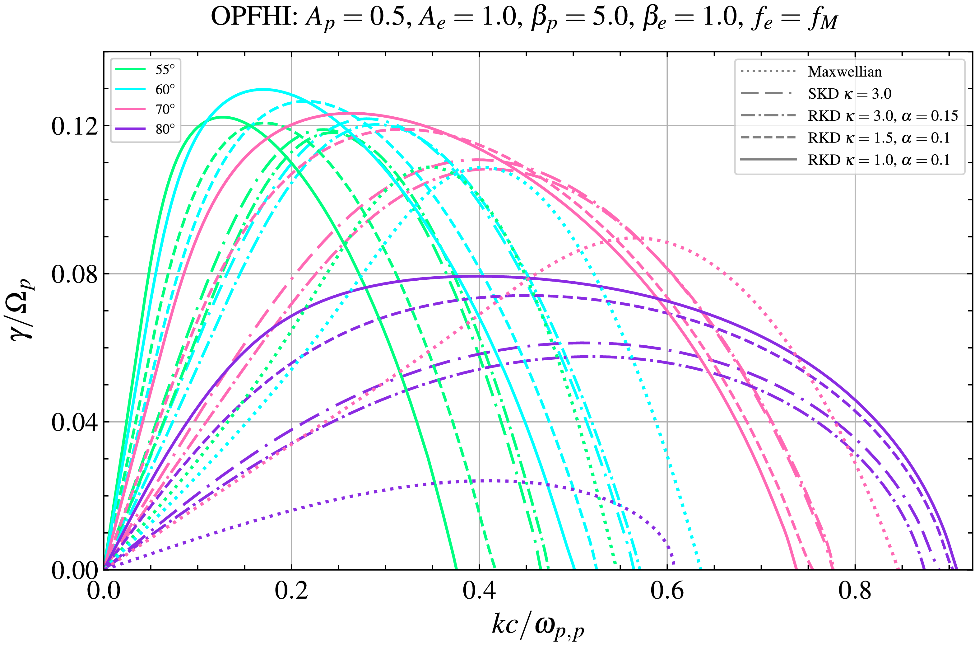
Figure 9 shows the normalised growth rates at higher propagation angles (
 $60^\circ$
,
 $70^\circ$
,
 $75^\circ$
and
 $80^\circ$
) for the Maxwellian and SKD cases and several RKDs, computed with ALPS. In this angular range, only unstable non-propagating modes are observed. The maximum growth rates in the RKD cases exceed those of the Maxwellian case at all angles. As
 $\kappa$
decreases,
 $\gamma _m$
increases and shifts toward lower
 $k_m$
. For example, at
 $\theta = 70^\circ$
, the RKD case with
 $\kappa = 1.0$
yields
 $\gamma _m/\varOmega _p = 0.1233$
at
 $k_m c/\omega _{pp} = 0.2629$
, which is approximately
 $38\,\%$
higher and corresponds to a
 $36\,\%$
reduction in
 $k_m$
compared with the Maxwellian case (
 $\gamma _m/\varOmega _p = 0.0897$
at
 $k_m c/\omega _{pp} = 0.4093$
). The RKD with
 $\kappa =3.0$
shows slightly lower maximum growth rates (up to
 $6\,\%$
) for all cases compared with the SKD, with differences becoming more pronounced at the highest angles, shifting the behaviour towards the solution of the Maxwellian VD.
As
 $\theta$
increases,
 $\gamma _m$
increases up to a maximum angle, while
 $k_m$
also increases and the peaks become significantly broader (particularly at
 $\theta = 80^\circ$
), extending over a wider interval of unstable wavenumbers. For all VDs, the maximum aperiodic growth rates remain below the corresponding maximum periodic growth rates in the parallel case. For instance, the Maxwellian case reaches its maximum aperiodic growth rate around
 $\theta = 55^\circ$
with
 $\gamma _m/\varOmega _p = 0.1088$
, which is approximately
 $12\,\%$
lower than the parallel value
 $\gamma _m/\varOmega _p = 0.123$
.
In all RKD cases, the maximum aperiodic growth rate is attained at slightly larger angles, around
 $\theta = 60^\circ$
. For example, for
 $\kappa = 1.0$
,
 $\gamma _m/\varOmega _p = 0.1298$
, which is approximately
 $23\,\%$
lower than the corresponding parallel value
 $\gamma _m/\varOmega _p = 0.169$
at
 $\theta = 0^\circ$
. At
 $\theta = 80^\circ$
, the RKD with
 $\kappa = 1.0$
exhibits a maximum growth rate that is approximately
 $229\,\%$
higher than in the Maxwellian case, along with an increase of about
 $50\,\%$
in the range of unstable wavenumbers.
Normalised growth rates as functions of the normalised wavenumber, for the (aperiodic) OPFHI at propagation angles
 $55^\circ$
,
 $60^\circ$
,
 $70^\circ$
and
 $80^\circ$
for Maxwellian and different RKDs.
4. Summary and outlook
In this work, we investigate the OEFHI and OPFHI in plasmas with VDs described by Maxwellians, by SKDs and, for the first time, by RKDs. The analysis extends previous studies of parallel propagation and provides a systematic comparison of the role of suprathermal particles for oblique wave propagation.
For the OEFHI, the validation against Li & Habbal (Reference Li and Habbal2000), while showing very good agreement between ALPS and DIS-K for Maxwellian plasmas, reveals systematic quantitative differences for oblique propagation. In particular, the present results consistently show an extension of the unstable wavenumber range and significantly enhanced growth rates for the periodic branch at intermediate angles. These differences lead to modified relative contributions of periodic and aperiodic branches, such that the significance of these modes can differ from earlier findings. The results presented here can therefore be regarded as an updated and more resolved reference for OEFHI in Maxwellian plasmas.
The comparison between Maxwellian, SKD and RKD plasmas reveals systematic trends. For parallel propagation, only periodic modes are present. Introducing suprathermal particles via SKDs enhances the growth rates and shifts the maxima toward lower wavenumbers. This trend becomes more pronounced for RKDs as
 $\kappa$
decreases, i.e. with increasing suprathermal particles, leading to sharper and more localised peaks in
 $k$
-space.
With increasing propagation angle, the behaviour becomes more complex due to the emergence of unstable aperiodic modes. For the Maxwellian case, the transition from periodic to aperiodic dominance already occurs at relatively small angles, and at intermediate angles the aperiodic branch can strongly dominate and exceed the growth rate of SKD and RKD. At larger angles, only non-propagating modes remain, with a pronounced maximum growth rate at highly oblique propagation.
In contrast, SKD and RKD plasmas show a ‘
 $\theta$
-delayed’ and weaker development of aperiodic modes. For small to intermediate angles, the periodic branch remains dominant in most cases, even when aperiodic contributions are present. As
 $\kappa$
is reduced, the periodic modes are systematically enhanced and shifted to lower wavenumbers, while the aperiodic modes become less pronounced or appear only at larger angles. There are also scenarios in which, at certain intermediate propagation angles, the aperiodic mode of a
 $\kappa$
-distribution attains a higher growth rate than both the periodic and aperiodic modes of a distribution with a lower
 $\kappa$
value, in contrast to the behaviour observed at smaller and larger angles: At highly oblique propagation, RKDs exhibit significantly enhanced growth rates compared with Maxwellian plasmas, with broader peaks and extended unstable wavenumber ranges. Notably, the maximum growth rate shifts to larger angles for lower
 $\kappa$
, and the overall growth rates become substantially increased by suprathermal effects. These growth rates would not be achievable using SKDs due to their limitation to
 $\kappa \gt 3/2.$
Compared with the periodic modes at parallel propagation, the aperiodic modes at higher angles are approximately two orders of a magnitude or more higher, making the latter more effective in regulating the free energy and thus reducing the anisotropy.
For the OPFHI, a qualitatively similar dependence on the VD is observed, but with important differences in the angular behaviour. In contrast to the OEFHI, the maximum growth rates are found for parallel propagation for both Maxwellian and SKD plasmas, as already shown in other studies and here also observed for RKDs. As the angle increases, the growth rates for the periodic solutions decrease and eventually only aperiodic modes remain. The inclusion of suprathermal particles again enhances the growth rates and shifts the maxima toward lower wavenumbers. This trend strengthens with decreasing
 $\kappa$
(for RKDs), leading to systematically higher growth rates than in the Maxwellian case at all angles. However, even at high obliqueness, the maximum growth rates of the aperiodic solutions remain below the corresponding values for the parallel (periodic) solutions.
While already shown for Maxwellian and SKDs, the OEFHI for RKDs with low-
 $\kappa$
transitions to aperiodic dominance at increased intermediate angles and exhibits its highest growth at oblique propagation. The growth rates for the OPFHI (with this set of plasma parameters) remain primarily dominated by periodic modes at parallel propagation, with aperiodic modes becoming relevant only at larger
 $\theta$
and never exceeding the parallel growth rates.
The comparison between the SKD with
 $\kappa =3$
and the corresponding RKD with
 $\kappa =3$
and
 $\alpha =0.15$
reveals that the cutoff generally shifts the solutions toward the Maxwellian case. For the OEFHI, this effect is particularly pronounced at intermediate propagation angles, where the suppression of the suprathermal tail enhances the relative importance of the aperiodic branch and can substantially increase its growth rate compared with the SKD case. At highly oblique propagation, however, the cutoff reduces the growth rates (of the aperiodic modes) and moves the instability closer to those of the Maxwellian plasma. Similar trends are found for the OPFHI.
The excellent agreement between ALPS and DIS-K demonstrates that ALPS is a reliable and flexible tool for studying oblique instabilities in plasmas with RKDs. This is particularly important since semi-analytical formulations for oblique propagation with RKDs are not yet available and numerical approaches remain essential for exploring their linear dispersion relations.
At the same time, the generation of contour maps in the
 $k-\theta $
-plane, which are valuable for identifying global maxima of the growth rate and for a systematic characterisation of oblique instabilities, is computationally more complex with ALPS compared with (semi-)analytic solutions. The development of semi-analytical expressions for oblique RKDs (analogous to those for isotropic RKDs derived by Gaelzer, Fichtner & Scherer Reference Gaelzer, Fichtner and Scherer2024), or improved numerical tools for efficiently obtaining these maps, would therefore be beneficial for future investigations.
Overall, the results demonstrate that suprathermal particles, as described by low-
 $\kappa$
RKDs, have a strong impact on the oblique firehose instabilities, modifying both the angular dependence of the maximum growth rate and the interplay between periodic and aperiodic modes. These effects, while to be expected, become indeed increasingly pronounced with lower
 $\kappa$
, scenarios which are inaccessible using SKDs, reflecting the role of suprathermal particles in enhancing the free energy available to drive kinetic instabilities. In this sense, the RKD adds the ability to actually realise and quantify this regime in a physically consistent way. The value of the present results, therefore, lies not only in the (anticipated) qualitative trend itself and not only in quantifying how the growth rates and unstable wavenumber ranges are enhanced once the low
 $\kappa$
regime becomes accessible, but more in demonstrating that this trend indeed persists for oblique propagation and for both the EFHI and PFHI.
Beyond the specific parameter choices explored here, these results are relevant for the interpretation of temperature-anisotropy constraints observed in the solar wind and other weakly collisional space and astrophysical plasmas, where suprathermal populations are ubiquitous and may be characterised by RKDs with low
 $\kappa$
values. The present work illustrates that physically consistent modelling of the low-
 $\kappa$
regime, made possible by the RKD, is not merely a technical refinement of the SKD but may have direct consequences for how kinetic instabilities are expected to constrain macroscopic plasma parameters in observational and simulation studies.
Acknowledgements
We gratefully acknowledge R.A. López for his ongoing support with DIS-K and for valuable discussions and technical assistance. The ALPS project received support from UCL’s Advanced Research Computing Centre through the Open Source Software Sustainability Funding scheme. This research was supported by the International Space Science Institute (ISSI) in Bern, through ISSI International Team project no. 612 (Excitation and Dissipation of Kinetic-Scale Fluctuations in Space Plasmas) led by K.G. Klein.
Editor Francesco Califano thanks the referees for their advice in evaluating this article.
Funding
The authors acknowledge support from the Ruhr-University Bochum and the Katholieke Universiteit Leuven. This project was funded by the Deutsche Forschungsgesellschaft (DFG, project FI
 $706/31$
-
 $1$
), the Belgian FWO-Vlaanderen (G
 $002523$
N) and SIDC Data Exploitation (ESA Prodex, No.
 $4000145223$
). D.V. is supported by STFC Consolidated Grant ST/W001004/1. K.G.K. was supported in part by NASA contract 80NSSC24K0171.
Declaration of interests
The authors report no conflict of interest.
Appendix A. Dispersion relation in ALPS
ALPS uses the general expression of the plasma’s susceptibilities (Verscharen et al. Reference Verscharen, Klein, Chandran, Stevens, Salem and Bale2018)
 \begin{align} \boldsymbol{\chi}_{\!j} & =\frac {\omega _{\mathrm{p}, j}^2}{\omega \varOmega _{j}} \int _0^{\infty } 2 \pi p_{\perp } \mathrm{d} p_{\perp } \int _{-\infty }^{+\infty } \mathrm{d} p_{\|}\Bigg [\hat {\boldsymbol{e}}_{\|} \hat {\boldsymbol{e}}_{\|} \frac {\varOmega _{j}}{\omega }\left (\frac {1}{p_{\|}} \frac {\partial f_{0 j}}{\partial p_{\|}}-\frac {1}{p_{\perp }} \frac {\partial f_{0 j}}{\partial p_{\perp }}\right ) p_{\|}^2 \nonumber\\[3pt]& \quad +\sum _{n=-\infty }^{+\infty } \frac {\varOmega _{j} p_{\perp } U}{\omega -k_{\|} v_{\|}-n \varOmega _{j}} \boldsymbol{T}_n\Bigg], \end{align}
where
 \begin{align} U \equiv \frac {\partial f_{0 j}}{\partial p_{\perp }}+\frac {k_{\|}}{\omega }\left (v_{\perp } \frac {\partial f_{0 j}}{\partial p_{\|}}-v_{\|} \frac {\partial f_{0 j}}{\partial p_{\perp }}\right ), \end{align}
 \begin{align} \boldsymbol{T}_n \equiv \begin{pmatrix} \dfrac {n^{2} J_n^{2}}{z^{2}} & \quad \dfrac {i n J_n J_n'}{z} & \quad \dfrac {n J_n^{2} p_{\|}}{z p_{\perp }} \\[15pt] -\dfrac {i n J_n J_n'}{z} & \quad \left (J_n'\right )^{2} & \quad -\dfrac {i J_n J_n' p_{\|}}{p_{\perp }} \\[15pt] \dfrac {n J_n^{2} p_{\|}}{z p_{\perp }} & \quad \dfrac {i J_n J_n' p_{\|}}{p_{\perp }} & \quad \dfrac {J_n^{2} p_{\|}^{2}}{p_{\perp }^{2}} \end{pmatrix}, \end{align}
where
 $z \equiv k_{\perp } v_{\perp } / \varOmega _{j}$
and
 $J_n \equiv J_n(z)$
denotes the
 $n$
th-order Bessel function. Using the plasma’s dielectric tensor as
 \begin{align} \boldsymbol{\epsilon } = \unicode {x1D7D9} + \sum _j \boldsymbol{\chi}_{\!j}, \end{align}
where
 $\unicode {x1D7D9}$
is the unity tensor, the wave equation can be written as in 1.9.
Appendix B. Validation and comparison of OEFHI solutions
Table 1 summarises the main quantitative differences between the present ALPS/DIS-K solutions and the OEFHI results previously reported by Li & Habbal (Reference Li and Habbal2000) for selected propagation angles, comparing the extent of the unstable wavenumber range, the location of the maximum growth rate and the relative dominance of periodic and aperiodic modes.
Normalised wave frequencies (left) and normalised growth rates (right) as functions of the normalised wavenumber for the OPFHI at different propagation angles. Results obtained with ALPS (solid lines) and DIS-K (dots). Top: Maxwellian distribution. Bottom: SKD with
 $\kappa =3.0$
.

Figure 10. Long description
The image contains four line graphs. Panel A and Panel B show results for a Maxwellian distribution, while Panel C and Panel D show results for an SKD distribution. Each panel compares results obtained with ALPS (solid lines) and DIS-K (dots). The x-axis in all panels represents the normalized wavenumber (kc/ωp,p). The y-axis in the left panels (A and C) represents the normalized wave frequency (ωr/Ωp), and the y-axis in the right panels (B and D) represents the normalized growth rate (γ/Ωp). Different colors represent different propagation angles, ranging from 0° to 80°. In Panel A and B, the lines for different angles overlap significantly, indicating similar behavior across angles for the Maxwellian distribution. In Panel C and D, the lines for different angles show more variation, indicating a dependence on the propagation angle for the SKD distribution.
Comparison between the OEFHI results reported by Li & Habbal (Reference Li and Habbal2000) and the present ALPS/DIS-K solutions for different propagation angles.
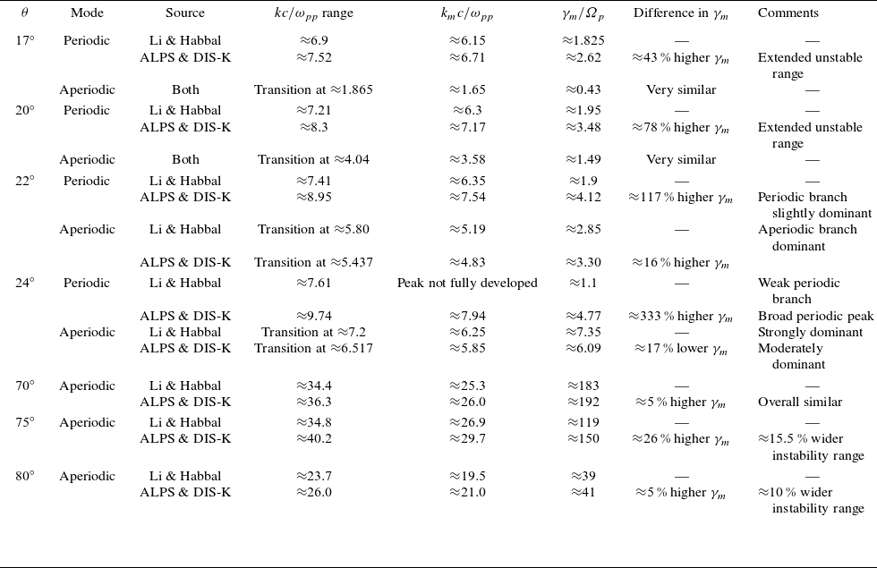
Table 1. Long description
Panel A: Line graph comparing OEFHI results and ALPS/DIS-K solutions for parallel propagation. The x-axis represents propagation angles in degrees, and the y-axis represents growth rates in percent. The graph shows excellent agreement between the two sets of results. Panel B: Line graph comparing OEFHI results and ALPS/DIS-K solutions for oblique propagation. The x-axis represents propagation angles in degrees, and the y-axis represents growth rates in percent. The graph shows noticeable differences between the two sets of results, with the present solutions exhibiting higher growth rates and larger ranges of unstable wavenumbers.
Appendix C. Validation. OPFHI with Maxwellian and SKD
Inspired by Hellinger & Matsumoto (Reference Hellinger and Matsumoto2000), we use Maxwellian protons with
 $\beta _{p}=5$
, and
 $T_{p,\perp }/T_{p,\|}=0.5$
, while electrons are described by an isotropic Maxwellian with
 $\beta _{e}=1$
. We extend this set-up by using an SKD with
 $\kappa = 3.0$
for the electrons. The results for different propagation angles are presented in figure 10, with the normalised frequency on the left-hand side and the normalised growth rate on the right-hand side (top panel: Maxwellian, bottom panel: SKD
 $\kappa = 3.0$
). The agreement between the two solvers is again very good (less than
 $0.1\,\%$
deviation for the Maxwellian cases and less than
 $0.4\,\%$
deviation for the SKD cases in terms of
 $\gamma _m$
and
 $k_m$
) and the findings (for the Maxwellian case) are very similar to those reported by Hellinger & Matsumoto (Reference Hellinger and Matsumoto2000). Contour plots of the OPFHI normalised frequency (left panel) and growth rate (right panel) in the
 $k$
–
 $\theta$
-plane for the Maxwellian case (top) and for the SKD with
 $\kappa =3.0$
(bottom) are shown in figure 11, revealing that for both Maxwellian and SKD the maximum growth rate is reached for parallel propagation. For a detailed discussion about the OPFHI, we refer the reader to Hellinger & Matsumoto (Reference Hellinger and Matsumoto2000) and Maneva et al. (Reference Maneva, Lazar, Viñas and Poedts2016).
Contour plot of the OPFHI normalised frequency (left panel) and growth rate (right panel) in the
 $k$
–
 $\theta$
-plane for the Maxwellian case (top) and SKD case with
 $\kappa =3.0$
(bottom), obtained with DIS-K.

Figure 11. Long description
The image contains four contour plots. Panel A and Panel B show the Maxwellian case, while Panel C and Panel D show the SKD case with kappa equals 3.0. Each panel is divided into two sub-panels: the left sub-panel displays the normalized frequency, and the right sub-panel displays the growth rate. The x-axis for all sub-panels is labeled ‘kc/ωpp’ and ranges from 0.0 to 0.8. The y-axis is labeled ‘θ’ and ranges from 0 to 80 degrees. The color scale at the top of each sub-panel indicates the magnitude of the normalized frequency or growth rate, with blue representing lower values and red representing higher values. In the Maxwellian case, the left sub-panels show non-propagating waves, while the right sub-panels distinguish between aperiodic and periodic regions. The SKD case with kappa equals 3.0 shows similar patterns but with different distributions of frequency and growth rate.
Appendix D. Maximum growth rates for OEFHI and OPFHI
The maximum growth rates
 $\gamma _{m}/\varOmega _p$
and the corresponding wavenumbers
 $k_m c/\omega _{pp}$
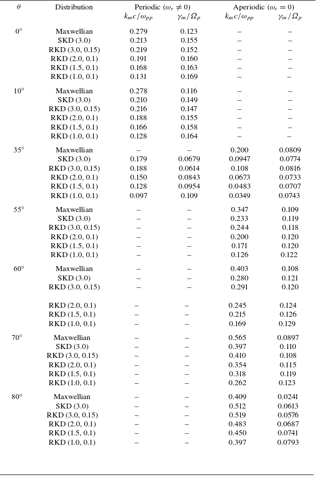
for the different cases are shown in table 2 for the OEFHI and in table 3 for the OPFHI.
Case of (O)EFHI: maximum growth rate
 $\gamma _{m}$
and corresponding wavenumber
 $k_{m}$
for Maxwellian, SKD and different RKDs
 $(\kappa , \alpha )$
and propagation angles
 $\theta$
. Modes are classified as periodic (
 $\omega _r \neq 0$
) or aperiodic (
 $\omega _r = 0$
).
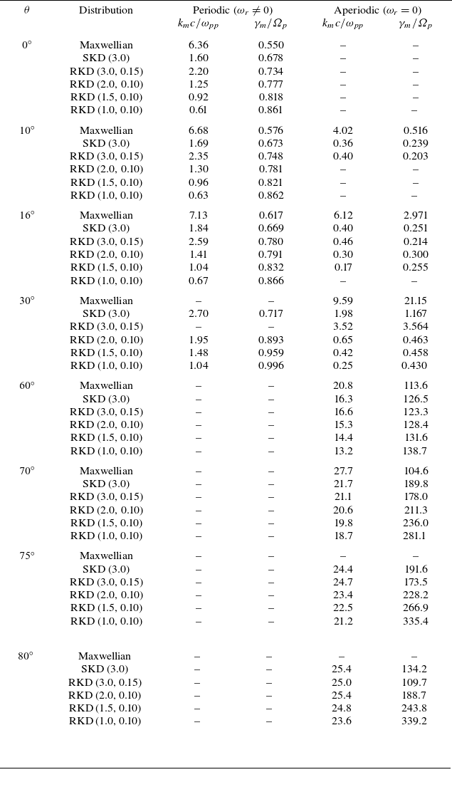
Table 2 Long description
A table comparing growth rates and wavenumbers for different plasma distributions and angles. The table has 10 rows and 7 columns. Column headers are: θ, Mode, Source, kc/wpp range, kmc/wpp, γm/Ωp, Difference in γm, Comments. Row 1: 17°, Periodic, Li & Habbal, ≈6.9, ≈6.15, ≈1.825, —, Extended unstable range. Row 2: 17°, Periodic, ALPS & DIS-K, ≈7.52, ≈6.71, ≈2.62, ≈43 % higher γm, Extended unstable range. Row 3: 17°, Aperiodic, Both, Transition at ≈1.865, ≈1.65, ≈0.43, Very similar, —. Row 4: 20°, Periodic, Li & Habbal, ≈7.21, ≈6.3, ≈1.95, —, —. Row 5: 20°, Periodic, ALPS & DIS-K, ≈8.3, ≈7.17, ≈3.48, ≈78 % higher γm, Extended unstable range. Row 6: 20°, Aperiodic, Both, Transition at ≈4.04, ≈3.58, ≈1.49, Very similar, —. Row 7: 22°, Periodic, Li & Habbal, ≈7.41, ≈6.35, ≈1.9, —, —. Row 8: 22°, Periodic, ALPS & DIS-K, ≈8.95, ≈7.54, ≈4.12, ≈117 % higher γm, Periodic branch slightly dominant. Row 9: 22°, Aperiodic, Li & Habbal, Transition at ≈5.80, ≈5.19, ≈2.85, —, Aperiodic branch dominant. Row 10: 22°, Aperiodic, ALPS & DIS-K, Transition at ≈5.437, ≈4.83, ≈3.30, ≈16 % higher γm, —. Row 11: 24°, Periodic, Li & Habbal, ≈7.61, Peak not fully developed, ≈1.1, —, Weak periodic branch. Row 12: 24°, Periodic, ALPS & DIS-K, ≈9.74, ≈7.94, ≈4.77, ≈333 % higher γm, Broad periodic peak. Row 13: 24°, Aperiodic, Li & Habbal, Transition at ≈7.2, ≈6.25, ≈7.35, —, Strongly dominant. Row 14: 24°, Aperiodic, ALPS & DIS-K, Transition at ≈6.517, ≈5.85, ≈6.09, ≈17 % lower γm, Moderately dominant. Row 15: 70°, Aperiodic, Li & Habbal, ≈34.4, ≈25.3, ≈183, —, —. Row 16: 70°, Aperiodic, ALPS & DIS-K, ≈36.3, ≈26.0, ≈192, ≈5 % higher γm, Overall similar. Row 17: 75°, Aperiodic, Li & Habbal, ≈34.8, ≈26.9, ≈119, —, —. Row 18: 75°, Aperiodic, ALPS & DIS-K, ≈40.2, ≈29.7, ≈150, ≈26 % higher γm, ≈15.5 % wider instability range. Row 19: 80°, Aperiodic, Li & Habbal, ≈23.7, ≈19.5, ≈39, —, —. Row 20: 80°, Aperiodic, ALPS & DIS-K, ≈26.0, ≈21.0, ≈41, ≈5 % higher γm, ≈10 % wider instability range.
Case of (O)PFHI: maximum growth rate
 $\gamma _{m}$
and corresponding wavenumber
 $k_{m}$
for Maxwellian, SKD and different RKDs
 $(\kappa , \alpha )$
and propagation angles
 $\theta$
. Modes are classified as periodic (
 $\omega _r \neq 0$
) or aperiodic (
 $\omega _r = 0$
).
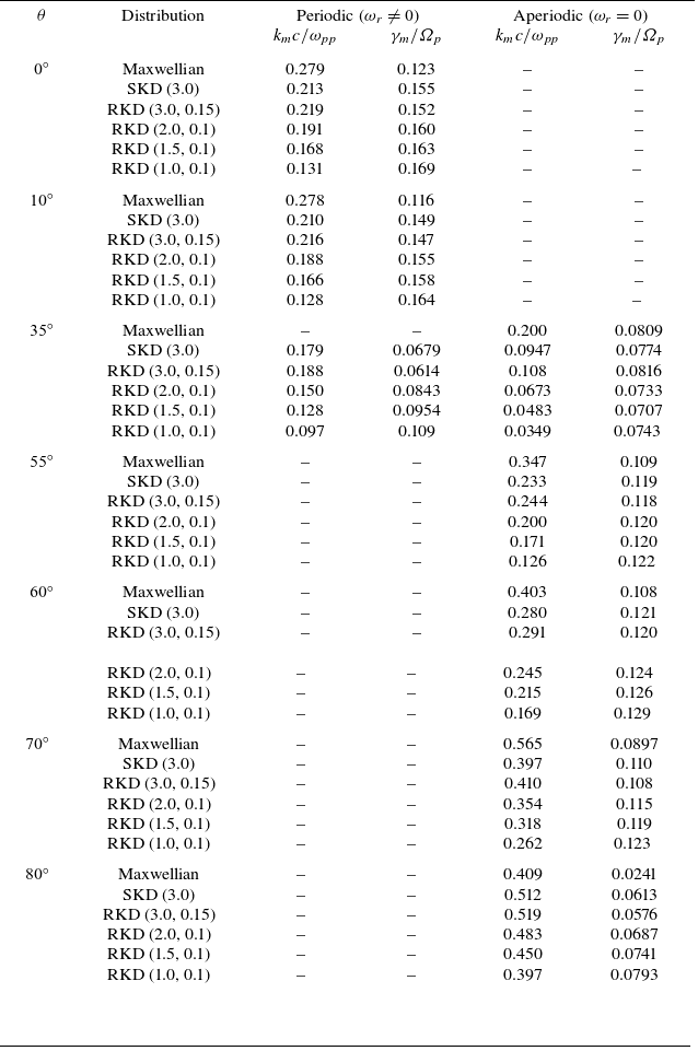
Table 3 Long description
Table 2: This table presents data for the OEFHI case. It includes columns for different conditions such as Maxwellian, SKD, and various RKDs, along with propagation angles. The table categorizes modes as periodic or aperiodic. Table 3: This table shows data for the OPFHI case, with similar columns and categorizations as Table 2.


 0∘
 17∘
 20∘
 22∘
 24∘

 30∘
 40∘
 50∘
 60∘
 70∘
 75∘
 80∘

 60∘
 70∘
 75∘
 80∘
 κ=3.0

 k
 θ
 κ=3.0

 0∘
 10∘
 16∘
 30∘

 16∘
 30∘

 60∘
 70∘
 75∘
 80∘

 0∘
 10∘
 35∘

 55∘
 60∘
 70∘
 80∘

 κ=3.0

 k
 θ
 κ=3.0
 γm
 km
 (κ,α)
 θ
 ωr≠0
 ωr=0
 γm
 km
 (κ,α)
 θ
 ωr≠0
 ωr=0

 Open access

