

Background
Climate change has had disastrous effects on agriculture and food security in many parts of the world, particularly in developing countries (IPCC 2007, 2014; World Bank, 2010). Among the many different sectors of the Bangladesh economy, crop agriculture is the most vulnerable to climate change (Government of Bangladesh, 2014). One major determinant of fluctuations in crop yield is year-to-year changes in climatic variables (Hazell, Reference Hazell1984; Anderson and Hazell, Reference Anderson and Hazell1987). Crop agriculture plays a vital role in the economy of Bangladesh. Agriculture contributes to 16.33% of the GDP and the crop subsector alone contributed 11% to GDP at constant prices in 2013–14 (Government of Bangladesh, 2014). Almost 85% of the rural population is directly or indirectly involved in agriculture. Of all crops, rice plays a leading role by contributing 95% of total food production (Government of Bangladesh, 2014). This paper is motivated by the importance of crop/rice sector's contribution to the Bangladesh economy, the sector's high vulnerability to climate change and existing limited studies, which draws these two issues together.
Rice, the main staple food in Bangladesh, is highly susceptible to climate change and climate related extreme events such as floods and droughts (Huq et al., Reference Huq, Ahmed, Koudstaal and Downing1996; Karim et al., Reference Karim, Hussain and Ahmed1996; Yu et al., Reference Yu, Alam, Hassan, Khan, Ruane, Rosenzweig, Major and Thurlow2010). Climate change, as has been estimated, will reduce rice production in Bangladesh on an average of 7.4% every year over the period 2005–2050 (Yu et al., Reference Yu, Alam, Hassan, Khan, Ruane, Rosenzweig, Major and Thurlow2010). However, there have been, to the best of our knowledge, no comprehensive studies of climate change by applying the panel data approach in Bangladesh. There are, of course, a few regional and national level studies on the impact of climate change and droughts on rural livelihoods and crop agriculture using descriptive statistics (Paul, Reference Paul1998; Rashid and Islam, Reference Rashid and Islam2007) and simulation models (Karim et al., Reference Karim, Hussain and Ahmed1996; Mahmood, Reference Mahmood1998; Mahmood et al., Reference Mahmood, Legates and Meo2004; Rimi et al., Reference Rimi, Rahman, Karmaker and Hussain2009; Basak, Reference Basak2010).
Three main rice crops, namely Aus, Aman and Boro, grow in three different seasons in Bangladesh. Aus is usually planted in March–April and harvested in June–July whilst Aman is usually sown in July–August and harvested in November–December. Finally, Boro is planted in December–January and harvested in May–June (Government of Bangladesh, 2014). Aus rice needs supplementary irrigation during the initial stage of its growing season while Aman is almost totally rain-dependent and is planted during the monsoon months, although it requires supplementary irrigation during planting and sometimes in the flowering stages depending on the availability of rainwater. Boro is totally irrigated as it grows in the dry winter and the hot summer (Mahmood, Reference Mahmood1998). This study is focused on Aman rice as it is rain-fed and more vulnerable to climate change (Alam, Reference Alam2015). Moreover, its contribution to total rice production is more than 40% covering nearly 50% of gross planted rice area.
This paper has the potential to contribute to the literature in some important ways. First, there are currently few empirical studies about climate change impact on mean crop yield and its variability (Chen et al., Reference Chen, McCarl and Schimmelpfennig2004; Isik and Devadoss, Reference Isik and Devadoss2006; Kim and Pang, Reference Kim and Pang2009; Sarker, Reference Sarker2012; Sarker et al., Reference Sarker, Alam and Gow2012a, Reference Sarker, Alam and Gow2013a, Reference Sarker, Alam and Gowb). These earlier studies using panel data have used only average temperature and average total rainfall as the two climate variables and average temperature was constructed as a mean of maximum temperature and minimum temperature. However, the addition of maximum and minimum temperature is only able to capture the differential impacts of day and night temperature (Peng et al., Reference Peng, Huang, Sheehy, Laza, Visperas and Zhong2004; Boomiraj et al., Reference Boomiraj, Chakrabarti, Aggarwal, Choudhary and Chander2010; Welch et al., Reference Welch, Vincent, Auffhammer, Moya, Dobermann and Dawe2010; Pattanayak and Kumar, Reference Pattanayak and Kumar2014). This study has employed both maximum and minimum temperature as temperature-related climate variables in the panel data framework. Secondly, past studies using panel data evaluated the impact of climate change on a particular crop (or a group of crops) as a whole (Chen et al., Reference Chen, McCarl and Schimmelpfennig2004; Deschenes and Greenstone, Reference Deschenes and Greenstone2007; Guiteras, Reference Guiteras2007; McCarl et al., Reference McCarl, Villavicencio and Wu2008; Schlenker and Roberts, Reference Schlenker and Roberts2008; Kim and Pang, Reference Kim and Pang2009; Barnwal and Kotani, Reference Barnwal and Kotani2010; Cabas et al., Reference Cabas, Weersink and Olale2010). However, different varieties of a crop are impacted differently by climate change (Isik and Devadoss, Reference Isik and Devadoss2006; Kabubo-Mariara and Karanja, Reference Kabubo-Mariara and Karanja2007; Sarker, Reference Sarker2012; Sarker et al., Reference Sarker, Alam and Gow2012a, Reference Sarker, Alam and Gowb, Reference Sarker, Alam and Gow2013a, Reference Sarker, Alam and Gowb; Sarker et al., Reference Sarker, Alam and Gow2014), which warrant crop-variety-specific research. Therefore, the objective of this study is to assess the impacts of climate change on the production of the Aman rice variety in Bangladesh over the period 1975–2012.
Materials and Methods
Theoretical framework
There have, internationally, been a number of studies measuring the effects of climate variables on crop productivity using either simulation models such as CERES-maize, CERES-rice or EPIC models (Phillips et al., Reference Phillips, Lee and Dodson1996; Mahmood, Reference Mahmood1998; Rosenzweig et al., Reference Rosenzweig, Tubiello, Goldberg, Mills and Bloomfield2002; Tan and Shibasaki, Reference Tan and Shibasaki2003; Mahmood et al., Reference Mahmood, Legates and Meo2004), or regression models (Mendelsohn et al., Reference Mendelsohn, Nordhaus and Shaw1994; Chang, Reference Chang2002; Haim et al., Reference Haim, Shechter and Berliner2008). In the main, two major theoretical frameworks were employed in these past studies to assess the impact of climate on agriculture: the production function approach (also known as crop modeling or agronomic models) (Mearns et al., Reference Mearns, Rosenzweig and Goldberg1997) and the Ricardian approach (Mendelsohn et al., Reference Mendelsohn, Nordhaus and Shaw1994). The first approach, based on controlled experiments, simulates data on climate factors and crop yields in a laboratory-type setting. With careful control and randomized application of environmental conditions, this approach has its capability to forecast the potential climatic impacts on agricultural yields. However, this approach does not take into consideration farmers’ attitudes toward adaptation and thus results in an overestimation of negative impacts and an underestimation of positive effects (Adams et al., Reference Adams, Rosenzweig, Peart, Ritchie, McCarl, Glyer, Curry, Jones, Boote and Allen1990, Reference Adams, Seinfeld and Koch1999; Mendelsohn et al., Reference Mendelsohn, Nordhaus and Shaw1994; Haim et al., Reference Haim, Shechter and Berliner2008).
The Ricardian approach estimates the relationship between land values and agro-climatic factors by making the use of cross-sectional data (Mendelsohn et al., Reference Mendelsohn, Nordhaus and Shaw1994; Kumar and Parikh, Reference Kumar, Parikh, Dinar, Mendelsohn, Everson, Parikh, Sanghi and Kumar1998). The main strength of this approach is that it captures farmers’ adaptations that affect land value as measured by net revenue or farm income. Consequently, the model has been successfully applied in a large number of countries: USA (Mendelsohn et al., Reference Mendelsohn, Nordhaus and Shaw1994); England and Wales (Maddison, Reference Maddison2000); Kenya (Kabubo-Mariara and Karanja, Reference Kabubo-Mariara and Karanja2007); Taiwan (Chang, Reference Chang2002); South Africa (Gbetibouo and Hassan, Reference Gbetibouo and Hassan2005); Cameroon (Molua, Reference Molua2009); China (Wang et al., Reference Wang, Mendelsohn, Dinar, Huang, Rozelle and Zhang2009); and India and Brazil (Sanghi and Mendelsohn, Reference Sanghi and Mendelsohn2008). However, the model, in its original form, cannot be applied to most developing countries because of the absence of efficient land markets and therefore accurate and observable land prices.
The major weakness of a Ricardian model lies in its inability to incorporate omitted variables such as the (unobservable) skill level of farmers and the quality of soil which are also known as time-independent and location specific factors (Barnwal and Kotani, Reference Barnwal and Kotani2010). However, variability in yield was found to be affected by climate variables in some studies (Chen et al., Reference Chen, McCarl and Schimmelpfennig2004; Chen and Chang, Reference Chen and Chang2005; Kim and Pang, Reference Kim and Pang2009).
The Ricardian model is unable to assess the effect of climate change on yield variability (Mearns et al., Reference Mearns, Rosenzweig and Goldberg1997). Nevertheless, this has already led some economists to use a panel data approach to take account of the omitted variables problem by including district or regional dummies in the model (Chen et al., Reference Chen, McCarl and Schimmelpfennig2004; Deschenes and Greenstone, Reference Deschenes and Greenstone2007; Guiteras, Reference Guiteras2007; McCarl et al., Reference McCarl, Villavicencio and Wu2008; Schlenker and Roberts, Reference Schlenker and Roberts2008; Kim and Pang, Reference Kim and Pang2009; Barnwal and Kotani, Reference Barnwal and Kotani2010; Cabas et al., Reference Cabas, Weersink and Olale2010). Moreover, panel data provides more information and degrees of freedom, and can control individual heterogeneity.
Furthermore, there are several other advantages in using a panel data approach such as the considerable increase in sample size, and it is better suited to the study of the dynamics of change by employing repeated cross-sectional observations (Gujarati, Reference Gujarati2004; Baltagi, Reference Baltagi2005). Previous studies are based on the framework of a Just and Pope (Reference Just and Pope1978) stochastic production function. Just and Pope (Reference Just and Pope1979) altered the traditional stochastic models of agricultural production processes to achieve more flexibility when dealing with risk. The basic concept of Just and Pope was to build a production function that is the sum of two parts: the standard mean output level and a term for the variability of output. Rain-dependant Aman rice is more vulnerable to climate variables and the different climate zones of Bangladesh are impacted differently by climate changes. To discern those effects, there is a need to assess the effects of climate variables on mean Aman rice yield and its variability in Bangladesh using district-level time series data grouped into seven climate zones.
Data, its sources and basic properties
This study uses cross-sectional time-series data for Aman rice from 13 greater districts in Bangladesh. The selection of districts was based on the availability of consistent data, on both climatic and rice yield. The districts included were Dhaka, Mymenshingh, Faridpur, Chittagong, Commilla, Bogra, Sylhet, Rajshahi, Dinajpur, Rangpur, Khulna, Jessore, and Barisal. District-level climate data for monthly maximum temperature, monthly minimum temperature and monthly total rainfall were collected from the Bangladesh Meteorological Department for 48 years covering the period 1964–2012. The monthly data were then used to group the climate variables into seasonal averages for temperature and seasonal totals for rainfall over each month of the growing season for Aman, which runs from July to December annually.
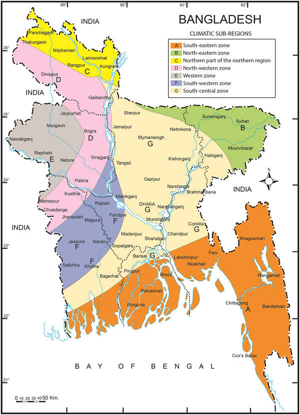
Data on Aman rice yield (measured in kilograms per acre (kg acre−1) were drawn from various issues of the Yearbook of Agricultural Statistical of Bangladesh for the period 1975–2012. The selection of the 13 districts, which are organized into seven climate zones was based on Rashid (Reference Rashid1991) which divided Bangladesh into seven climatic sub-zones (Fig. 1). These sub-zones are described briefly:
Climate zone map of Bangladesh.

Southeastern zone (A): This zone consists of the greater Chittagong district and Chittagong Hill Tracts and a coastal strip extending from southwest Sundarban to the south of Comilla. Heavy rainfall and small range of mean temperature are the major climatic characteristics of this region.
Northeastern zone (B): This zone comprises the greater Sylhet district. The salient climatic features of this region include mild summer temperatures, heavy rainfall and a cloudy cold winter.
Northern part of the northern zone (C): This zone includes the greater Rangpur district and the northern part of the greater Dinajpur district. In terms of climate, this is an area of extremes: heavy rainfall, hot summer temperatures and cold winters are three major climatic characteristics.
Figure 1 depicts the different climate zones and selected district(s) under each zone.
Northwestern zone (D): This area consists Dinajpur, Bogra, Pabna and Kushtia districts. The main climatic conditions are hot summer temperatures and moderate rainfall.
Western zone (E): This is the driest and hottest sub-zone, which includes the greater Rajshahi districts and parts of adjacent districts. Very hot summer temperatures and relatively low rainfall are the climatic features of this zone. This is the area of interest for the farm level analysis.
Southwestern zone (F): This zone comprises Khulna, Jessore and Faridpur districts with fewer extremes in both temperature and rainfall. Climatic characteristics are hot summer temperatures and fairly heavy rainfall.
South central zone (G): This is an area of mild summers and fairly heavy rainfall. This zone consists of Dhaka, Tangail, Mymensingh and Barisal districts.
The summary statistics on rice yield and climate variables are illustrated in Table 1 which shows a number of basic properties of the variables in the form of some descriptive statistics. Also higher means are associated with higher standard deviations: the correlation coefficient of values for means and standard deviations is 0.996 and significant at the 0.01 level. With regard to the climate variables, the variations in rainfall are more remarkable than the variations in both maximum and minimum temperatures.
Summary statistics for Aman yield and climate variables.

Note: T max, maximum temperature; T min, minimum temperature; R, rainfall.
Empirical model specification
In order to determine the effects of climate variables on the level of yield and its variability, the stochastic production function approach pioneered by Just and Pope (Reference Just and Pope1978, Reference Just and Pope1979) is applied. The fundamental concept underpinning this approach is that the production function can be decomposed into two segments: the first segment is linked to the mean output level while the second segment is associated with the variability of that output (Kim and Pang, Reference Kim and Pang2009; Cabas et al., Reference Cabas, Weersink and Olale2010). This function thus allows inputs to be either risk-increasing or risk-decreasing (Koundouri and Nauges, Reference Koundouri and Nauges2005). The general form of the Just and Pope Production function is (Just and Pope, Reference Just and Pope1978):
 $$y = f\,(X) + h(X)\epsilon, $$
where y is yield and X is a set of explanatory variables. The parameter estimation of f(X) provides the average impact of the explanatory variables on yield, while h(X) offers their effect on the variability of yield (Chen and Chang, Reference Chen and Chang2005). Based on Saha et al. (Reference Saha, Havenner and Talpaz1997) and Chen et al. (Reference Chen, McCarl and Schimmelpfennig2004) we estimate a production function of the following form:
 $$y = f\,(x) + u = f\,(X,\alpha ) + h\; (X,\beta )\epsilon, $$
where y is Aman rice yield, X is a set of explanatory variables (e.g. temperature, rainfall, location and time period) and ε is an exogenous production shock with E(ε) = 0 and  ${\rm Var}({\epsilon} ) = \delta _{\epsilon} ^2 $. With this formulation, explanatory variables affect both the mean and variability of rice yield because E(y) = f(x) and Var(y) = Var(u) = h(.). The parameter estimation of f(.) gives the average effects of the explanatory variables on yield, while h(.) reveals the impacts of the covariates on the variability of yield. It is noteworthy that a positive sign on any parameter of h(.) implies that a rise in that variable indicates an increase of the variability of yield. On the other hand, negative sign in the same function indicates a variability decreasing indicating that weather variables are risk reducing.
Three functional forms of production functions: Cobb–Douglas, quadratic and translog are commonly used in estimating Just and Pope production functions (Tveteras, Reference Tveteras1999; Chen et al., Reference Chen, McCarl and Schimmelpfennig2004; Isik and Devadoss, Reference Isik and Devadoss2006; Kim and Pang, Reference Kim and Pang2009). Because of the multiplicative interaction between the mean and variance, a translog functional form would violate the Just and Pope postulates (Tveteras, Reference Tveteras1999, Reference Tveteras2000; Koundouri and Nauges, Reference Koundouri and Nauges2005). Therefore, we selected Cobb–Douglas and linear quadratic forms for the mean yield function estimation. These two forms are consistent with the Just and Pope postulates (Tveteras, Reference Tveteras2000; Kim and Pang, Reference Kim and Pang2009).
Mean function
The mean function is specified as:
Cobb–Douglas form: 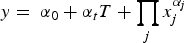 $y = \; \alpha _0 + \alpha _tT + \mathop \prod \limits_j x_j^{\alpha _j} $
Linear-Quadratic Form:
 $$y = \; \alpha _0 + \alpha _tT + \mathop \sum \limits_j \alpha _{1j}x_j + \; \mathop \sum \limits_j \alpha _{2j}x_j^2 + \mathop \sum \limits_j \mathop \sum \limits_{k(k \ne j)} \alpha _{jk}x_jx_k$$
where x j and x ke are explanatory variables that include weather variables, T is the time trend, which has potential to reveal the effects of technological advances such as new crop varieties and improved cropping practices; and α′s are coefficients to be estimated. The justification of including a time trend is that it can capture technological progress over the period under consideration.
Variance function
Following Just and Pope (Reference Just and Pope1978, Reference Just and Pope1979), Kumbhakar and Tveteras (Reference Kumbhakar and Tveteras2003) and Koundouri and Nauges (Reference Koundouri and Nauges2005), the variability function h(.) in (1) and (2) is modeled thus:
 $${\rm Cobb} \hbox{-} {\rm Douglas}\;\hbox{form\colon}\ h(x) = \beta _0T\mathop \prod \limits_j x_j^{\beta _j} $$
where β′s are parameters to be estimated.
With respect to risk, the Just–Pope production function is more informative than traditional production functions because it contains an additional component. The first component explains the impact of inputs on mean/expected output whilst the second one makes clear the effects of inputs on variability of output (Just and Pope; Reference Just and Pope1978, Reference Just and Pope1979).
Fixed effect and random effect models are usually used for a panel model (Baltagi, Reference Baltagi2005). This study used the fixed effect model purposely for two reasons. First, this model allows for climate zone-specific characteristics to take into account the regional differences in the mean yield function. Secondly, it is appropriate in situations where there is a possibility of correlation between regressors and time-invariant distinctiveness as is the case here. On the other hand, the random effects model necessitates the assumption of no correlation between the unobserved time-invariant characteristics and the explanatory variables. Therefore, the fixed effect model is selected for this study and this selection is consistent with its use in similar past studies (McCarl et al., Reference McCarl, Villavicencio and Wu2008; Kim and Pang, Reference Kim and Pang2009; Barnwal and Kotani, Reference Barnwal and Kotani2010; Cabas et al., Reference Cabas, Weersink and Olale2010).
Estimation method
Both maximum likelihood estimation (MLE) and three-step feasible generalized least squares (FGLS) were prescribed in Just and Pope (Reference Just and Pope1978, Reference Just and Pope1979) for estimating both functional forms. However, FGLS estimation is employed in most empirical studies, although MLE is more efficient and unbiased than FGLS for small samples (Saha et al., Reference Saha, Havenner and Talpaz1997). Given the large sample size here, FGLS was finally used, as described in Judge et al. (Reference Judge, Griffiths, Hill, Lutkepohl and Lee1985), to estimate a form of fixed effects panel model. It is noteworthy that both FGLS and MLE were used in our preliminary analyses but FGLS was found to produce the better results in terms of both statistical and economic significance of the parameters of the variables used. Furthermore, FGLS appeared better than MLE in terms of overall significance of the model. This is another reason for the choice of FGLS as an estimation method. Additionally, the problems of heteroscedasticity and auto-correlation are better tackled in FGLS (Gujarati, Reference Gujarati2004; Cameron and Trevedi, Reference Cameron and Trevedi2009).
Panel unit roots and stationarity
It is essential to investigate the presence of unit roots for each potential variable before we estimate the model. This is true for both the FGLS and MLE methods. One important assumption of the Just and Pope model is that the variables under estimation are stationary (Chen et al., Reference Chen, McCarl and Schimmelpfennig2004). Therefore, variables having the properties of I(1) must be differenced before panel estimation occurs (McCarl et al., Reference McCarl, Villavicencio and Wu2008). Otherwise, using a non-stationary data set directly might yield spurious results (Granger and Newbold, Reference Granger and Newbold1974; Chen and Chang, Reference Chen and Chang2005). However, the time series properties of one variable comprising many regions/areas in a panel data setting are hard to characterize (Chen et al., Reference Chen, McCarl and Schimmelpfennig2004). Several versions of the panel unit root test are available in the literature. This study uses the Fisher-type test as proposed in Maddala and Wu (Reference Maddala and Wu1999). The Fisher test obtains more precise results and achieves higher power compared with other potential tests (Barnwal and Kotani, Reference Barnwal and Kotani2010).
Fisher-type test
Maddala and Wu (Reference Maddala and Wu1999) and Choi (Reference Choi2001) proposed a test, which combines the P-values from individual unit root tests. If π i is defined as the P-value from any individual unit root test for cross-section section i, under the null of unit root, then, for all N cross-sections, the asymptotic result we use is:
 $$- 2\mathop \sum \limits_{i = 1}^N {\rm ln}(\pi _i) \to 2N.$$
The advantage of this Fisher-type test is that it can be used for different lag lengths in individual ADF regressions and can be used with many other unit root tests (Baltagi, Reference Baltagi2005). Moreover, the Fisher type-test used in conjunction with regression and bootstrap-based values performs the best. Consequently it is the preferred method for testing non-stationarity in panel data (Maddala and Wu, Reference Maddala and Wu1999).
The hypotheses of the Fisher-type test are: H o: All panels contain unit roots; H a: At least one panel is stationary.
Results and Discussion
Results from the panel unit root test
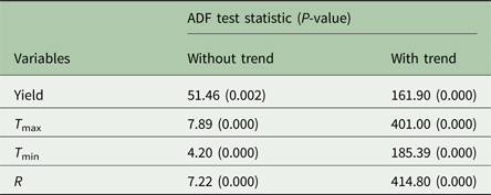
The Fisher-type test is used to examine the stationarity properties of the variables in a panel model. There are two versions of the Fisher-type test: ADF (Augmented Dickey Fuller) and PP (Philips and Perron) tests. This study obtained identical results from these two versions and reproduces the results using ADF only in Table 2.
Panel unit root test results.

Note: Hypothesis under ADF test: H o, all panels contain unit roots; H a, at least one panel is stationary.
Hypothesis under PP test: H o, panels contain unit roots; H a, panels are stationary.
The estimated test statistics imply that rice yields and climate variables exhibit similar results both with and without a time trend. This suggests that the null hypothesis of unit roots (i.e. non-stationary) is rejected at the 1% level of significance for all variables in the table. This implies that all variables under the model are stationary. These results are consistent with McCarl et al. (Reference McCarl, Villavicencio and Wu2008); and Kim and Pang (Reference Kim and Pang2009). Therefore, the three-stage FGLS method can be applied to analyze the data without differencing.
Results from the empirical model
Estimates of the Cobb–Douglas and quadratic functions for mean yield and yield variability are made using the FGLS estimation method. Regional dummies are included for the mean yield function but not for the variability function. This assumes different regions have different mean yields with almost identical variances across zones. We have included six regional dummies for the seven climate zones to avoid the dummy variable perfect collinearity trap (Gujarati, Reference Gujarati2004).
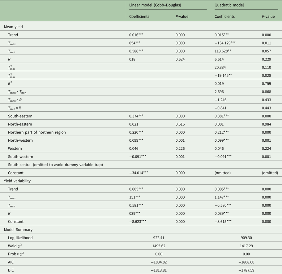
The impact of climate change on rice yield is reported in Table 3. Since the Wald statistic of 1495.62 has a P-value of 0.000 for the linear functional form and the P-value of Wald statistics for the quadratic functional form is also 0.000; the regressors under both the functional forms are, as a whole, statistically significant. This implies that the regressors are jointly significant. The values of the Akaike Information Criterion (AIC) and Bayesian Information Criterion (BIC) are used to select the better functional form. The linear Cobb–Douglas functional form is better because it has the highest negative value. The sign and level of significance for the mean yield impacts of climate variables for Aman rice are not the same between the linear and quadratic functional forms. The maximum temperature has a positive impact on the mean yields in the linear model and a negative effect in the quadratic model. On the other hand, minimum temperature has a negative effect on rice yield in the linear model while a positive impact in the quadratic model. Finally, rainfall is not statistically significant in either functional form. In the quadratic function, the quadratic term for minimum temperature is statistically significant with a negative effect on Aman rice yield. The other two quadratic terms are not statistically significant. None of the three interaction terms are statistically significant.
Aman rice estimation results.

Note: ***, ** and * represent levels of significant at 1, 5 and 10%, respectively.
All of the regional dummies are statistically significant in both functional forms aside from the north-eastern and western zones. Moreover, most of the significant regions have a positive impact on yield except south-western, which has a negative effect.
From the viewpoint of the yield variability function, the effects of maximum temperature and rainfall on rice yield variability are positive and statistically significant. On the contrary, the impact of minimum temperature on rice yield is negative with statistical significance. This implies that higher minimum temperature is risk-decreasing while higher maximum temperature and increased rainfall are risk-increasing. Finally, the trend variable has a positive impact on rice yield and variability under both functional forms.
Climate elasticities of Aman rice yield
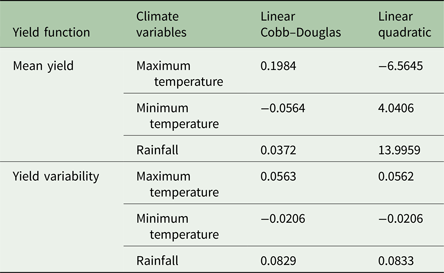
Since the quadratic models have both quadratic and interaction terms, it is not possible to contrast the signs and extent of the estimated coefficients in the quadratic function to those in the linear function. The estimation of elasticities, which gives a common denominator is used to assess and compare the effects of climate variables both in the linear Cobb–Douglas and linear-Quadratic functional forms and are calculated at the mean values of the explanatory variables (Isik and Devadoss, Reference Isik and Devadoss2006). The coefficients for climate variables such as maximum temperature, minimum temperature and rainfall can be translated into elasticities through multiplying by the average of the climate variable and dividing by average yield (Chen et al., Reference Chen, McCarl and Schimmelpfennig2004). These elasticities are reported in Table 4. The estimated elasticities are different, to some extent, between linear and quadratic function for mean yield while the values for elasticities are slightly different in the variance function.
Aman rice elasticities of climate variables.

The elasticity of maximum temperature is computed as 0.1984 and −6.5645 in the mean yield function. Therefore, a 1% increase in maximum temperature level usually increases the mean yield by 0.20% in the Cobb–Douglas form while it is decreased by 6.56% under the linear quadratic function. Minimum temperature has a negative impact on the mean yield in Cobb–Douglas form while it affects mean yield positively in the linear quadratic model. The elasticity for rainfall is estimated at 0.04 and 13.99, which implies a 1% rise in rainfall increases mean yield by 0.04–14%.
Maximum temperature and higher rainfall increase the variability of Aman rice. A 1% increase in maximum temperature causes yield variability to rise by 0.06% whilst a 1% increase in rainfall increases yield variability by 0.08%. However, minimum temperature has a negative impact on the variability of rice yield and a 1% increase in minimum temperature results in a decline in yield variability by 0.02%. Therefore, maximum temperature and rainfall are risk increasing while minimum temperature is risk-decreasing for Aman rice.
Effects of future climate change
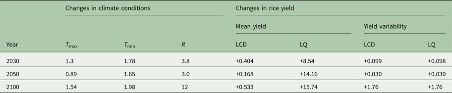
The estimated elasticities are now used to estimate the impacts of future climate change scenarios on rice yield and its variability. In so doing, a few climate change scenarios are modeled (Ministry of Environment and Forests, 2005, 2009). The changes in rice yields for each climate scenario are measured using percentage changes in maximum temperature, minimum temperature and rainfall together with the estimates of elasticities. The percentage changes in mean yield and variance for 2030, 2050 and 2100 are presented in Table 5.
Change in mean Aman yield and yield variability (%).

Note: T max, temperature maximum; T min, temperature minimum; R, rainfall; LCD, linear Cobb–Douglas; LQ, linear quadratic.
These data indicate that all three scenarios of climate change would result in an increase in mean rice yield in both the linear and quadratic functions. However, the mean yield increase in the linear quadratic (LQ) function is well above the value for the linear Cobb–Douglas (LCD) function. It would be expected that future climate changes would expand yield variability over the years and the variations are profound when comparing 2030 with 2100. However, the percentage variability changes are very similar in both functional forms.
The Just–Pope production function results in superior estimates compared with more traditional production functions. However, there are some caveats to this in that the model is limited to the first two moments of the output distribution, input levels are likely to be endogenous in estimation, risk preferences are unidentified and price risk is not taken into consideration.
Conclusions and Policy Implications
Climate change will have potential effects on the mean and variability of crop yields. The main aim of this study was to evaluate the effects of climate changes on the yield and variability for Aman rice using regionally disaggregated data. The Just–Pope production function was used as the empirical framework in a balanced panel data specification to achieve the aim. Maximum temperature is positively related to Aman mean rice yield in the linear function while the relationship is negative in the quadratic function. The elasticity values under the variance function imply that maximum temperature is risk-increasing for Aman rice. However, an increase in minimum temperature is likely to decrease the yield variability. Therefore, minimum temperature is risk-decreasing for Aman rice. Finally, the impacts of rainfall on yield variability are positive for Aman rice. This confirms that rainfall is risk-increasing for Aman rice. Three time scenarios (2030, 2050 and 2100) were developed to model potential climate changes on rice yield and its variability. The changes in rice yield for each of these scenarios were measured using the percentage changes in maximum temperature, minimum temperature and rainfall in an aggregate form. The results reveal that future climate change is expected to increase the variability of Aman rice yield.
These results provide further evidence about the potential productivity losses, which will occur with future changes in climate variables. Moreover, most of the regional dummy variables are statistically significant with differential impacts geographically on rice yield. This shows that different climate zones can be impacted differently by climate change. Therefore, the severity of climate change effects on rice yields may vary between climate zones.
These results caution against adopting country or state-level adaptation policies, which may be ineffective. Our results suggest that region-specific or climate zone specific adaptation policies should be implemented. This then warrants the need for more location-specific research on climate change and agricultural production. This will enable the development of local or micro-level adaptation policies for reducing yield variability, and ensuring food security in the presence of climate change.
Finally, one caveat to be mentioned is that although the panel data model is an improvement over time series or cross-sectional data; the model does not always provide a cure-for-all for all of the econometrician's problems (Gujarati, Reference Gujarati2004). For example, how individual farmers are affected by climate change is not discernable from the panel model results. Despite this, the impacts of climate change are predominantly more profound at the farm-level (Downing, Reference Downing1992). Moreover, climate zone-level panel data does not include farmers’ adaptation strategies, which are vital to overcoming the adverse effects of climate change. Data from farmer surveys, thus, can more explicitly outline the effects of climate change and climate related extreme events. Future studies, therefore, should focus on the analysis of climate change impact and adaptation at the farm-level.
Author Contributions
RS conceived the study, undertook the initial analysis and approved the final manuscript; KA wrote the original draft of the manuscript and checked the final manuscript; and JG checked the analysis and wrote the final version of the manuscript.
Acknowledgements
The authors would like to thank the anonymous reviewers and the editor for their suggestions which immeasurably improved the paper.