Introduction
Due to its remoteness and extreme weather and sea conditions, the Southern Ocean (SO) is a challenging region in which to carry out biological studies (Kaiser et al. Reference Kaiser, Brandão, Brix, Barnes, Bowden and Ingels2013, Gutt et al. Reference Gutt, Isla, Bertler, Bodeker, Bracegirdle and Cavanagh2017). It is also one of Earth's regions where we observe the most rapid and dramatic environmental changes in marine ecosystems, motivating the study of these marine communities (Turner et al. Reference Turner, Barrand, Bracegirdle, Convey, Hodgson and Jarvis2014, Ashton et al. Reference Ashton, Morley, Barnes, Clark and Peck2017, Clark et al. Reference Clark, Nieva, Hoffman, Davies, Trivedi and Turner2019). Ecological modelling approaches are now well established and can be used to predict spatial patterns of organisms', populations’ and species’ distributions and assess their environmental drivers (Peterson et al. Reference Peterson, Soberón, Pearson, Anderson, Martínez-Meyer, Nakamura and Araújo2011). Based on field observations and experimental datasets, ecological modelling encompasses valuable approaches to helping to analyse biological data and interpolating our knowledge of species distributions in relation to environmental descriptors (Kennicutt et al. Reference Kennicutt, Chown, Cassano, Liggett, Massom and Peck2014).
Species distribution models (SDMs) are ecological models that study the statistical relationship between species occurrence records and environmental factors, determining the set of environmental conditions that is suitable to a species distribution (Elith et al. Reference Elith, Graham, Anderson, Dudík, Ferrier and Guisan2006, Elith & Leathwick Reference Elith and Leathwick2009, Peterson et al. Reference Peterson, Soberón, Pearson, Anderson, Martínez-Meyer, Nakamura and Araújo2011). They represent the species realized niche (Pearson Reference Pearson2007, Sillero Reference Sillero2011), being the ensemble of abiotic conditions in which the species survives and reproduces, adding into consideration the influence of biotic interactions (competition, predation, parasitism, symbiosis, etc.) (Hutchinson Reference Hutchinson1957). SDMs have been widely used in various fields of ecology, such as conservation biology, biogeography, palaeoecology and global change biology (Pearson Reference Pearson2007). In recent years, a growing number of ecological studies have used SDMs to analyse the distribution of marine pelagic and benthic species in the SO (e.g. marine invertebrates, fish, seabirds and marine mammals) and to determine species environmental preferences (Loots et al. Reference Loots, Koubbi and Duhamel2007, Pierrat et al. Reference Pierrat, Saucède, Laffont, De Ridder, Festeau and David2012, Xavier et al. Reference Xavier, Raymond, Jones and Griffiths2016, Nachtsheim et al. Reference Nachtsheim, Jerosch, Hagen, Plötz and Bornemann2017), to compare ecological niche predictions in response to changing environments (Basher & Costello Reference Basher and Costello2016, Gallego et al. Reference Gallego, Dennis, Basher, Lavery and Sewell2017, Guillaumot et al. Reference Guillaumot, Fabri-Ruiz, Martin, Eléaume, Danis, Féral and Saucède2018b, Jerosch et al. Reference Jerosch, Scharf, Deregibus, Campana, Zacher and Pehlke2019) or to identify diversity hotspots for conservation purposes (Pinkerton et al. Reference Pinkerton, Smith, Raymond, Hosie, Sharp, Leathwick and Bradford-Grieve2010, Hibberd Reference Hibberd2016, Thiers et al. Reference Thiers, Delord, Bost, Guinet and Weimerskirch2017).
However, the quality of ocean-wide models is often limited by the heterogeneity, amount and spatial distribution of data, along with limited temporal and spatial resolutions. For all of these reasons, both modelling methods and model construction should be tested for accuracy and robustness prior to interpretation, and these indicators should be transparently communicated to ensure that model outputs are relevant given the specificities of the datasets used for modelling.
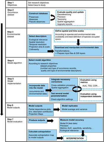
In the present paper, we review the most common methodological issues encountered in species distribution modelling applied to the SO, following the flowchart in Fig. 1. Challenges regarding occurrence and environmental dataset peculiarities are described. The choice of SDM algorithm and procedures to implement and evaluate models are addressed. Based on benthic invertebrate case studies, we stress important precautions to take and pitfalls to avoid during common steps of SDM implementation. Finally, we aim to provide some guidelines with a set of potential methods and original solutions that can be used for improving model performance.
Flow chart of the species distribution model construction process. Steps 1–4 concern data collection and treatment. Steps 5–7 integrate procedures for model implementation and validation. Dashed rectangles allow for a possible step backwards when assessing model uncertainties or evaluating model performance. AUC = area under the receiver operating curve; COR = Pearson correlation; GIS - Georeferencing Information System; TSS = true skill statistic.

Quality of datasets
Environmental datasets: field data
Preparing environmental datasets is the first encountered challenge when generating models (Gutt et al. Reference Gutt, Zurell, Bracegridle, Cheung, Clark and Convey2012, De Broyer et al. Reference De Broyer, Koubbi, Griffiths, Raymond, d'Udekem d'Acoz and Van de Putte2014). The SO, here defined as waters south of 45°S latitude, covers an extensive area of > 20 million km2 (Breitzke Reference Breitzke2014). Having access to environmental data with good temporal and spatial resolutions at such a broad scale is challenging, an issue common to all broad-scale oceanographic studies (Robinson et al. Reference Robinson, Nelson, Costello, Sutherland and Lundquist2017). ‘Broad scale’ is defined here as the entire SO, ‘regional scale’ as smaller areas of a few hundred square kilometres and ‘local scale’ as a few square kilometres to square metres (Gage Reference Gage2004).
Oceanographic data acquisition in the field is strongly conditioned by weather and sea conditions along with the seasonality of polar regions (polar night and dense sea-ice coverage in winter) that prompt recurring gaps in the acquisition of environmental data in the SO. Data are also much more frequently sampled close to research stations and along main sailing routes (Guillaumot et al. Reference Guillaumot, Artois, Saucède, Demoustier, Moreau and Eléaume2019). This is particularly striking in regions such as the south-western Weddell Sea, along the shores of the western Antarctic Peninsula and in the Bellingshausen and Amundsen seas (Clarke et al. Reference Clarke, Griffiths, Linse, Barnes and Crame2007, Griffiths et al. Reference Griffiths, Van de Putte, Danis, De Broyer, Koubbi, Griffiths, Raymond and Udekem d'Acoz2014).
Environmental datasets: satellite-derived data
Satellite-derived data form a significant source of information for SO oceanographic studies. Providing valuable environmental indicators at broad spatial scale, they can give details about continuous and long-term measurements of water masses including sea-ice coverage, extent and duration, sea-surface temperatures and salinities, biogeochemical parameters, sea level, primary production and typical meteorological parameters (El Mahrad et al. Reference El Mahrad, Newton, Icely, Kacimi, Abalansa and Snoussi2020).
The accuracy of satellite data, however, should be considered with care, given detection limits, interpolations that reduce the influence of atmospheric particulate scatter and the use of interpolation and gap-filling methods that smooth raw data at broad spatial and temporal scales (Pope et al. Reference Pope, Wagner, Johnson, Shutler, Baeseman and Newman2017, Stock et al. Reference Stock, Subramaniam, Van Dijken, Wedding, Arrigo and Mills2020).
Whenever possible, it is recommended to validate environmental data derived from satellite products at regional and local scales by comparing pixels on a satellite image with ‘real’ field observation data (Henson et al. Reference Henson, Yool and Sanders2015, Trull et al. Reference Trull, Passmore, Davies, Smit, Berry and Tilbrook2018). Simple correlation analyses or more complex ground-truth processes are available to compare satellite and in situ data and to secure the interpretation of satellite-derived products (White-Newsome et al. Reference White-Newsome, Brines, Brown, Dvonch, Gronlund and Zhang2013, Allan Reference Allan2014). This, however, constitutes a huge task and is not performed generally before implementing SDMs.
Environmental datasets: access to datasets
Environmental data generated at the scale of the entire SO can be accessed for free through different web portals such as the NASA's OceanColor Web (https://oceancolor.gsfc.nasa.gov), where satellite-derived data, averaging different temporal measurements down to 4 km resolution, are available at the scale of the entire SO dating from 2000. These images are post-processed to characterize sea-surface temperature or ocean colour as proxies of surface productivity.
The National Oceanic and Atmospheric Administration's (NOAA) data centre (WOCE2013; https://www.nodc.noaa.gov/OC5/woa13/woa13data.html) also makes available post-processed data of ocean temperature, salinity, oxygen concentration and nutrients at different grid formats, down to 0.25° resolution, averaging over six decades (from 1955 to 2012). Bio-ORACLE (https://www.bio-oracle.org) compiles a large panel of marine data layers at 1° spatial resolution for different depth layers and time periods, for the present (2005–2012) and the future (2040–2050; 2090–2100) (Assis et al. Reference Assis, Tyberghein, Bosch, Verbruggen, Serrão and De Clerck2018). Finally, GEBCO (https://www.gebco.net) is the reference platform for very-high-resolution bathymetry data (~500 m resolution) of the world's oceans.
Several works also make available compilations of these SO datasets dedicated to ecological modelling in the SO; they represent a valuable source of information for starting data preparation and modelling (https://data.aad.gov.au/metadata/records/Polar_Environmental_Data, https://data.aad.gov.au/metadata/records/fulldisplay/environmental_layers, https://data.aad.gov.au/metadata/records/Environmental_data_Southern_Ocean).
An increasing amount of environmental data collected during SO oceanographic campaigns have been made accessible for regional-scale studies. Several web portals aggregate all of these field measurements and provide them open access (e.g. https://www.marine-geo.org/collections/#!/collection/USAP#summary; https://www.pangaea.de).
Environmental datasets: spatial and temporal resolutions
Most environmental data are accessible through broad-scale maps from the aforementioned data portals and are available with a finest spatial resolution of ~4 km, if not coarser (https://data.aad.gov.au/metadata/records/Polar_Environmental_Data, De Broyer et al. Reference De Broyer, Koubbi, Griffiths, Raymond, d'Udekem d'Acoz and Van de Putte2014, https://data.aad.gov.au/metadata/records/fulldisplay/environmental_layers, https://data.aad.gov.au/metadata/records/Environmental_data_Southern_Ocean). This low resolution strongly hampers the precise assessment of relationships between species occurrences and environmental descriptors (Pittman Reference Pittman2017, Staveley et al. Reference Staveley, Perry, Lindborg and Gullström2017) and consequently the accuracy of model predictions (Connor et al. Reference Connor, Hull, Viña, Shortridge, Tang and Zhang2018), because the relevance of environmental descriptors represents a trade-off between their resolution and their spatial and temporal coverage (Guisan et al. Reference Guisan, Graham, Elith and Huettmann2007, Seo et al. Reference Seo, Thorne, Hannah and Thuiller2009, Lauzeral et al. Reference Lauzeral, Grenouillet and Brosse2013, Vale et al. Reference Vale, Tarroso and Brito2014). It is recommended that the resolution of environmental descriptors used in SDM should be in line with the scale of ecological processes at play and for which species ecophysiological responses show the highest variations, if models are expected to capture most species-environment relationships (Austin & Van Niel Reference Austin and Van Niel2011).
The published environmental datasets are often averaged over relatively long periods of time (from years to decades for WOCE2013 or Bio-ORACLE). The analysis of inter-annual variations can complement the interpretation of model predictions: the absence of such information does not preclude running models, but this should be kept in mind when it comes to interpreting model outputs (Guillaumot et al. Reference Guillaumot, Martin, Eléaume and Saucède2018a). Important environmental variations within a reference time period may not satisfy the equilibrium criterion between species distribution and environmental conditions, which is a strong prerequisite of SDM (Elith et al. Reference Elith, Graham, Anderson, Dudík, Ferrier and Guisan2006) and may affect the relevance and accuracy of model predictions (Guillaumot et al. Reference Guillaumot, Martin, Eléaume and Saucède2018a). In this respect, an alternative for improving modelling performance would be using seasonal averages or extreme values as environmental descriptors rather than pluri-annual to annual averages (Franklin Reference Franklin2009, Bradie & Leung Reference Bradie and Leung2017).
Environmental datasets: cartographic projections
Considering the poles in numerical analyses has long been a source of difficulty in spatial modelling as the convergence of meridians distorts shapes, surfaces, angles or distances towards high latitudes when using standard cylindrical representations such as the Mercator projection (Deleersnijder et al. Reference Deleersnijder, Van Ypersele and Campin1993, Eby & Holloway Reference Eby and Holloway1994, Murray Reference Murray1996). Working with conical or azimuthal projections (e.g. polar stereographic system) helps maintain the consistency of angles and shapes and therefore better meets the requirements of SO studies, although areas and distances are progressively distorted when moving away from the pole (Mulcahy & Clarke Reference Mulcahy and Clarke2001).
Mapping environmental descriptors and projecting model predictions can be carried out with either square or hexagonal pixels. Each option does not alter image quality and hexagonal shapes may even offer some advantages (Kamgar-Parsi & Sander Reference Kamgar-Parsi and Sander1989, Tirunelveli et al. Reference Tirunelveli, Gordon and Pistorius2002). However, some contrasts may be present between images using square or hexagonal pixels, as each pixel measures the average environmental conditions in the considered surface (Vanden Berghe et al. Reference Vanden Berghe2013).
Subdividing the study area into sub-regions and using different pixel shapes can be a good solution for improving the relevance of representations (Vanden Berghe et al. Reference Vanden Berghe2013, M. Cryer, unpublished data 2015). Evaluating the accuracy of environmental values captured both in square and hexagonal pixels using baseline in situ field measurements can also be suggested. This is yet to be tested for ecological modelling studies for the SO.
Environmental datasets: future forecasts
Since 1992, future climate models have been constantly updated through the efforts of the Coupled Model Intercomparison Projects (CMIP) featured by the Intergovernmental Panel on Climate Change (IPCC) Assessment Reports (ARs) with the aim of providing a plausible representation of future climate linked to potential anthropogenic impacts (https://www.ipcc.ch/site/assets/uploads/2018/03/sres-en.pdf, Mearns et al. Reference Mearns, Hulme, Carter, Leemans, Lal and Whetton2001). Recent updates (CMIP5 and CMIP6) of climate models are driven by different possible future greenhouse gas emission scenarios (Representative Concentration Pathways RCP2.6, RCP4.5, RCP6.0 and RCP8.5, from the least to the most pessimistic scenario for CMIP5, and Shared Socioeconomic Pathways SSP1 to SSP5 for CMIP6) and are built upon the average of an ensemble of simulations (Hayhoe et al. Reference Hayhoe, Edmonds, Kopp, LeGrande, Sanderson, Wehner, Wuebbles, Wuebbles, Fahey, Hibbard, Dokken, Stewart and Maycock2017). Future climate models for the SO are available through two main online platforms: Bio-ORACLE (https://www.bio-oracle.org; Assis et al. Reference Assis, Tyberghein, Bosch, Verbruggen, Serrão and De Clerck2018) and the NOAA's portal (https://psl.noaa.gov/ipcc/ocn).
The relevance of using future predictions based on global assessment scenarios for marine studies has been widely questioned (Flato et al. Reference Flato, Marotzke, Abiodun, Braconnot, Chou and Collins2014, Frölicher et al. Reference Frölicher, Rodgers, Stock and Cheung2016, de la Hoz et al. Reference De la Hoz, Ramos, Acevedo, Puente, Losada and Juanes2018), including their use in SDMs, given that climate models mainly rely on untestable assumptions (Beaumont et al. Reference Beaumont, Hughes and Pitman2008, Gotelli & Stanton-Geddes Reference Gotelli and Stanton-Geddes2015, Cavanagh et al. Reference Cavanagh, Murphy, Bracegirdle, Turner, Knowland and Corney2017, Freer et al. Reference Freer, Partridge, Tarling, Collins and Genner2018), future layers are not always available for oceanographic studies (Fabri-Ruiz Reference Fabri-Ruiz2018, Guillaumot et al. Reference Guillaumot, Martin, Eléaume and Saucède2018a, Reference Guillaumot, Fabri-Ruiz, Martin, Eléaume, Danis, Féral and Saucède2018b), discrepancies between present observations and future predictions can be problematic (Jiménez-Valverde et al. Reference Jiménez-Valverde, Rodríguez-Rey and Peña-Aguilera2021) and models are based on a representation of the climate system that has a complex cascading effect on ecological processes (Cavanagh et al. Reference Cavanagh, Murphy, Bracegirdle, Turner, Knowland and Corney2017). Cavanagh et al. (Reference Cavanagh, Murphy, Bracegirdle, Turner, Knowland and Corney2017) examined how well IPCC-class models reproduced sea-ice conditions. By subsetting CMIP5 models that best describe spatial extent and temporal ice cover, they improved the precision of the projected future sea-ice distribution, which was better suited to ecological analyses. Extending this method to other key oceanographic parameters should contribute to improving the accuracy of future climate models for the SO and their relevance to ecological studies.
Occurrence datasets: historical compilation
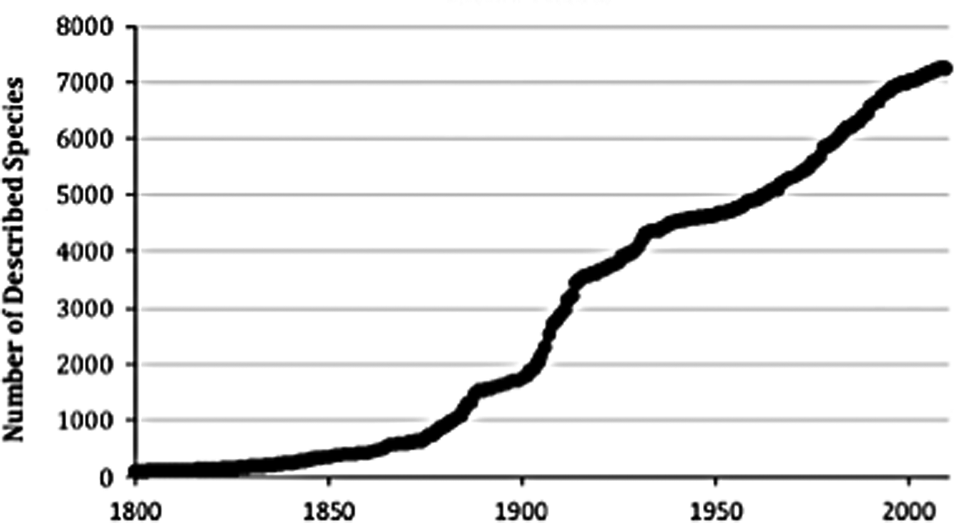
Biological sampling in the SO began with the first expeditions of the HMS Challenger (1873–1876). Sampling effort has considerably increased over the second part of the twentieth century and during recent decades in particular, following technological advances that have enabled the access to remote regions and sample processing (Fig. 2).
Cumulative number of Antarctic species described over time, according to data available in the Register of Antarctic Marine species (until March 2010). From De Broyer & Danis (Reference De Broyer and Danis2011).

This long-lasting and irregular effort in biogeographical (occurrence) data collection has had an impact on data compilation and has resulted in heterogeneous datasets, as observed in several data papers and associated Integrated Publishing Toolkit (IPT) databases such as Guillaumot et al. (Reference Guillaumot, Martin, Fabri-Ruiz, Eléaume and Saucède2016), Fabri-Ruiz et al. (Reference Fabri-Ruiz, Saucède, Danis and David2017) or Moreau et al. (Reference Moreau, Mah, Agüera, Améziane, Barnes and Crokaert2018), or in the general platform biodiversity.aq web portal.
The historical compilation of biological data includes 1) taxon misidentifications and taxonomic inconsistencies due to the various taxonomic revisions published through time, 2) errors in the georeferencing of occurrence records due to contrasting nomenclatures used to report latitude and longitude, 3) the accumulation of errors in metadata through the different generations of curation and 4) errors due to the use of different coordinate projection systems. Finally, in cases where species distributions may have shifted with time, species environmental preferences may have changed or non-contemporaneous environmental or occurrence datasets are used, discrepancies between occurrence records and environmental conditions can be present and violate the environment-occurrence equilibrium assumption necessary to generate SDMs. All of these side effects were reviewed in detail by Newbold (Reference Newbold2010). The impacts on species niche definition and SDM predictions have been reported in many works (Ensing et al. Reference Ensing, Moffat and Pither2012, Lahoz-Monfort et al. Reference Lahoz-Monfort, Guillera-Arroita and Wintle2014, Monk Reference Monk2014, Aguiar et al. Reference Aguiar, da Rosa, Jones and Machado2015, Tessarolo et al. Reference Tessarolo, Ladle, Rangel and Hortal2017, Guillaumot et al. Reference Guillaumot, Martin, Eléaume and Saucède2018a) that all advise us to thoroughly check datasets for quality management prior to running models.
Occurrence datasets: spatial aggregation
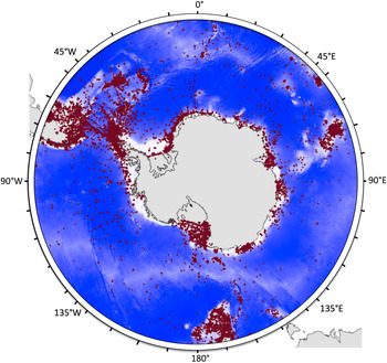
Most species occurrence data were collected in the vicinity of research bases or their surroundings or along recurrent maritime routes, leading to clear spatial aggregation patterns in biological datasets (Fig. 3) (Griffiths et al. Reference Griffiths, Van de Putte, Danis, De Broyer, Koubbi, Griffiths, Raymond and Udekem d'Acoz2014, Guillaumot et al. Reference Guillaumot, Artois, Saucède, Demoustier, Moreau and Eléaume2019).
Distribution of benthos sampling sites (red dots) in the Southern Ocean (SO, < 45°S). Sampling sites are not evenly distributed in the SO, showing important spatial aggregation in the Scotia Arc region and Western Antarctic Peninsula with several clusters along the Antarctic shelf, and over the Kerguelen and Campbell plateaus. In contrast, deep-sea regions and remote areas of the Antarctic shelf are under-sampled. From Guillaumot et al. (Reference Guillaumot, Artois, Saucède, Demoustier, Moreau and Eléaume2019), updated from Griffiths et al. (Reference Griffiths, Van de Putte, Danis, De Broyer, Koubbi, Griffiths, Raymond and Udekem d'Acoz2014).

Spatial aggregation can affect model accuracy, as aggregated presence records do not fully and homogeneously represent the entire environment that is occupied by given species. This aggregation also violates an initial assumption of SDMs that requires independence between records (Araújo & Guisan Reference Araújo and Guisan2006, Hijman Reference Hijmans2012). This may bias model predictions (Luoto et al. Reference Luoto, Pöyry, Heikkinen and Saarinen2005, Segurado et al. Reference Segurado, Araujo and Kunin2006, Dormann Reference Dormann2007, Kühn Reference Kühn2007, Crase et al. Reference Crase, Liedloff and Wintle2012), leading to statistical artefacts and generating inaccurate patterns (Bahn & McGill Reference Bahn and McGill2007, Currie Reference Currie2007).
Spatial aggregation of data and the effect of this spatial aggregation on model outputs can be quantified using the Moran's I index, which estimates the spatial autocorrelation between the presence records used to build the model and predicted presence probabilities (Luoto et al. Reference Luoto, Pöyry, Heikkinen and Saarinen2005). This spatial autocorrelation implies that close pixels are expected to present more similar predicted probabilities than distant ones due to the short geographical distance between records rather than environmental similarities alone. Testing and correcting for this bias should help to reduce its impact on model predictions (see the ‘Correcting spatial biases’ section) (Diniz-Filho et al. Reference Diniz-Filho, Bini and Hawkins2003, Kühn Reference Kühn2007).
Occurrence datasets: presence-only records
SDMs based on presence/absence data are recognized as having better predictive performance than models using presence-only data (Zaniewski et al. Reference Zaniewski, Lehmann and Overton2002, Brotons et al. Reference Brotons, Thuiller, Araújo and Hirzel2004, Wisz & Guisan Reference Wisz and Guisan2009, Lobo et al. Reference Lobo, Jiménez-Valverde and Hortal2010, Smith Reference Smith2013, Carvalho et al. Reference Carvalho, Rangel, Ready and Vale2015, Peel et al. Reference Peel, Hill, Foster, Wotherspoon, Ghiglione and Schiaparelli2019). However, except for some local-scale studies (e.g. Robinson et al. Reference Robinson, Elith, Hobday, Pearson, Kendall, Possingham and Richardson2011), in most oceanographic studies species absence records are usually not available for SDMs, and working with presence-only records is the only alternative (Lobo et al. Reference Lobo, Jiménez-Valverde and Hortal2010). SDMs are then built by associating presence-only records with a random selection of background records that will be used to characterize the full environmental conditions (Franklin Reference Franklin2010, Barbet-Massin et al. Reference Barbet-Massin, Jiguet, Albert and Thuiller2012). Background records should not be mistaken for pseudo-absence records that are artificial absence data, where the species is supposed (but not confirmed) to be absent. Pseudo-absence records do not represent the overall conditions of the study area. Presence/pseudo-absence models represent another modelling approach, predicting occupied and unoccupied habitats rather than suitable and less suitable habitats for presence/background modelling (Sillero & Barbosa Reference Sillero and Barbosa2021).
Presence-only datasets may contain several uncertainties that can bias model predictions. 1) Working on rare or cryptic species is generally prone to taxonomic misidentifications that may either contract or, alternatively, expand the extent of predicted species distributions (Costa et al. Reference Costa, Foody, Jiménez and Silva2015, Aubry et al. Reference Aubry, Raley and McKelvey2017). Such biases due to taxonomic errors were shown to be highly variable and to depend on experts identifying specimens, as suggested by Beale & Lennon (Reference Beale and Lennon2012), who worked on a compilation of several collections. 2) Sampling gear may have an impact on species detection. Inaccurate species observations may generate false-positive results (species predicted as being present when they were not sampled or observed in the field) and false-negative results (species predicted as being absent when they were sampled or observed in the field) during model initialization (Guillera-Arroita Reference Guillera-Arroita2016). Species presence records should be carefully scrutinized prior to modelling (Lozier et al. Reference Lozier, Aniello and Hickerson2009), or at least records should be categorized into different subsets of data verifiability (Aubry et al. Reference Aubry, Raley and McKelvey2017). 3) Georeferencing errors are a frequent issue in databases (Murphey et al. Reference Murphey, Guralnick, Glaubitz, Neufeld and Ryan2004, Maldonaldo et al. Reference Maldonado, Molina, Zizka, Persson, Taylor and Albán2015). This is especially the case in large databases compiling independent datasets using species presences recorded with varying levels of precision (Graham et al. Reference Graham, Elith, Hijmans, Guisan, Townsend Peterson and Loiselle2008, Bloom et al. Reference Bloom, Flower and DeChaine2018). Several studies have simulated virtual random georeferencing errors and have shown that these errors lead to significant drops in model performance and inconsistencies in the respective contributions of environmental descriptor contributions, influencing model interpretation (Graham et al. Reference Graham, Elith, Hijmans, Guisan, Townsend Peterson and Loiselle2008, Osborne & Leitão Reference Osborne and Leitão2009, Naimi et al. Reference Naimi, Skidmore, Groen and Hamm2011). These side effects seem to be minimized in local-scale models, here again advocating for the use of local-scale models whenever possible (Mitchell et al. Reference Mitchell, Monk and Laurenson2017).
Occurrence datasets: dealing with small datasets
Usually, the number of species presence records available for modelling is relatively limited considering the wide geographical extent of the SO (De Broyer et al. Reference De Broyer, Koubbi, Griffiths, Raymond, d'Udekem d'Acoz and Van de Putte2014). Generating SDMs with small datasets may include many pitfalls: 1) It reduces the potential of SDMs to transfer in space and time (Hernandez et al. Reference Hernandez, Graham, Master and Albert2006, Raes Reference Raes2012), 2) it truncates predicted distribution and niche definition (Hortal et al. Reference Hortal, Lobo and Jiménez-Valverde2007, Reference Hortal, Jiménez-Valverde, Gómez, Lobo and Baselga2008, Rocchini et al. Reference Rocchini, Hortal, Lengyel, Lobo, Jimenez-Valverde and Ricotta2011, Sánchez-Fernández et al. Reference Sánchez-Fernández, Lobo and Hernández-Manrique2011, Titeux et al. Reference Titeux, Maes, Van Daele, Onkelinx, Heikkinen and Romo2017, El-Gabbas & Dormann Reference El-Gabbas and Dormann2018), 3) it reduces modelling goodness-of-fit as the model may wrongly represent reality (Stockwell & Peterson Reference Stockwell and Peterson2002, McPherson et al. Reference McPherson, Jetz and Rogers2004, Pearson et al. Reference Pearson, Raxworthy, Nakamura and Townsend Peterson2007, Wisz et al. Reference Wisz, Hijmans, Li, Peterson, Graham and Guisan2008, Liu et al. Reference Liu, Newell and White2019), 4) it increases instability between model replicates (Guillaumot et al. Reference Guillaumot, Martin, Eléaume and Saucède2018a), 5) it gives rise to methodological constraints on threshold selection (Jiménez-Valverde & Lobo Reference Jiménez-Valverde and Lobo2007, Bean et al. Reference Bean, Stafford and Brashares2012), 6) it gives rise to methodological constraints on the application of evaluation metrics (Pearson et al. Reference Pearson, Raxworthy, Nakamura and Townsend Peterson2007), 7) it complicates the identification of model optimal complexity (Galante et al. Reference Galante, Alade, Muscarella, Jansa, Goodman and Anderson2018) and 8) it leads to a reduction in model accuracy because presence and background datasets would not differ markedly (Luoto et al. Reference Luoto, Pöyry, Heikkinen and Saarinen2005).
Alternatives are being developed to produce more accurate models based on a limited amount of presence records. One solution is generating several models performed on restricted areas and datasets with more detailed information and then averaging them with a weighted ensemble approach. This ‘ensemble of small models’ approach showed improved performance compared to single models (Lomba et al. Reference Lomba, Pellissier, Randin, Vicente, Moreira, Honrado and Guisan2010, Breiner et al. Reference Breiner, Guisan, Bergamini and Nobis2015, Reference Breiner, Nobis, Bergamini and Guisan2018).
Another alternative is to restrict the prediction area according to where occurrence records are found and ensuring upstream that the number of records is sufficient to precisely characterize the species environmental preferences: trivial advice that is surprisingly neglected, as recently pointed out by Morales et al. (Reference Morales, Fernández and Baca-González2017) and Araújo et al. (Reference Araújo, Anderson, Barbosa, Beale, Dormann and Early2019).
Occurrence datasets: definition of species-occupied environmental space
Spatial aggregation, along with heterogeneity, limited size and uncertainties in datasets, can strongly bias the quantification of the species-occupied environmental space (Hortal et al. Reference Hortal, Jiménez-Valverde, Gómez, Lobo and Baselga2008, Newbold Reference Newbold2010, Tessarolo et al. Reference Tessarolo, Ladle, Rangel and Hortal2017). However, accurately defining species-occupied space is the cornerstone of SDM initialization (Elith et al. Reference Elith, Graham, Anderson, Dudík, Ferrier and Guisan2006, Boulanger et al. Reference Boulanger, Parisien and Wang2018).
Moreover, SDMs suppose that species are in equilibrium with the environmental conditions that they inhabit. SDMs do not take into consideration potential vagrants that have dispersed out of their usual environmental range or populations that could momentarily survive in unsuitable habitats because doing so violates the equilibrium assumption between species distribution and environmental conditions (Beale & Lennon Reference Beale and Lennon2012). These elements should be cautiously considered when preparing datasets prior to generating models by removing any atypical records.
Over the last two decades, field data acquisition has expanded through the use of biologging technology with electronic devices attached to seabirds and marine mammals in order to access the positions of species all year long (Raymond et al. Reference Raymond, Lea, Patterson, Andrews-Goff, Sharples and Charrassin2015, Ropert-Coudert et al. Reference Ropert-Coudert, Van de Putte, Reisinger, Bornemann, Charrassin and Costa2020). These data uncover the hidden behaviours of marine animals and constitute a powerful way of better estimating species-occupied space; they can also be used to validate and refine our understanding of the environmental conditions prevailing in those species distribution areas (Arthur et al. Reference Arthur, Hindell, Bester, De Bruyn, Trathan, Goebel and Lea2017, Nachtsheim et al. Reference Nachtsheim, Jerosch, Hagen, Plötz and Bornemann2017, Hindell et al. Reference Hindell, Reisinger, Ropert-Coudert, Hückstädt, Trathan and Bornemann2020).
Adapting model implementation to datasets
The choice of modelling algorithms
To run performant SDMs, several assumptions must be tested and computing methods adapted to each case study (Austin Reference Austin2002, de la Hoz et al. Reference De la Hoz, Ramos, Puente and Juanes2019). Among them, the choice of the modelling algorithm should be of major concern, as no algorithm works best for all species, in all areas, at all spatial scales and in all time periods (Jarnevich et al. Reference Jarnevich, Stohlgren, Kumar, Morisette and Holcombe2015, Qiao et al. Reference Qiao, Soberón and Peterson2015). The selection and parameterization of modelling algorithms proved to be major causes of variation between SDM predictions (Dormann et al. Reference Dormann, Purschke, Márquez, Lautenbach and Schröder2008, Diniz-Filho et al. Reference Diniz-Filho, Mauricio Bini, Fernando Rangel, Loyola, Hof, Nogués-Bravo and Araújo2009, Buisson et al. Reference Buisson, Thuiller, Casajus, Lek and Grenouillet2010, Watling et al. Reference Watling, Brandt, Bucklin, Fujisaki, Mazzotti, Romañach and Speroterra2015, Boulanger et al. Reference Boulanger, Parisien and Wang2018). Each algorithm is particularly suited for dealing with a specific type and quality of data (Guisan & Zimmermann Reference Guisan and Zimmermann2000, Austin Reference Austin2002, Elith et al. Reference Elith, Graham, Anderson, Dudík, Ferrier and Guisan2006, Peterson Reference Peterson, Soberón, Pearson, Anderson, Martínez-Meyer, Nakamura and Araújo2011, Guisan et al. Reference Guisan, Thuiller and Zimmermann2017), which will determine the final model outputs (Aguirre-Gutiérrez et al. Reference Aguirre-Gutiérrez, Carvalheiro, Polce, van Loon, Raes, Reemer and Biesmeijer2013, Beaumont et al. Reference Beaumont, Graham, Duursma, Wilson, Cabrelli and Baumgartner2016).
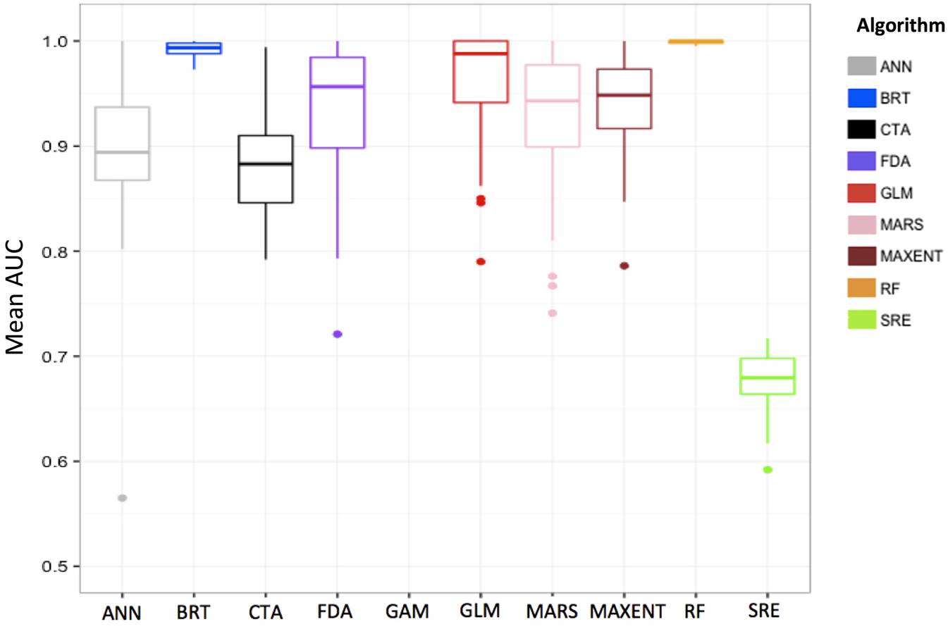
When modelling species distribution, it is necessary to select appropriate algorithms that have good transferability performances (i.e. have good abilities to correctly transfer predictions to other geographic space and time periods; Randin et al. Reference Randin, Dirnböck, Dullinger, Zimmermann, Zappa and Guisan2006) and that they limit overfitting (i.e. mitigate model complexity) while being flexible in integrating complex environmental relationships. Machine-learning algorithms (e.g. maximum entropy (MaxEnt), boosted regression trees (BRTs), random forests (RFs), support vector machines (SVMs); Vapnik Reference Vapnik1998, Breiman Reference Breiman2001, Elith et al. Reference Elith, Leathwick and Hastie2008, Reference Elith, Phillips, Hastie, Dudík, Chee and Yates2011) give access to important aspects of computing performance (Zhou Reference Zhou2012) and are relevant approaches for handling complex relationships between species occurrences and the environment (Olden et al. Reference Olden, Lawler and Poff2008, Elith & Leathwick Reference Elith and Leathwick2009). The BRT and RF algorithms are particularly suited to complex and heterogeneous datasets (Fig. 4; Guillaumot et al. Reference Guillaumot, Danis and Saucède2020a). They were proven to be efficient in generating performant models with limited overfitting (Elith et al. Reference Elith, Graham, Anderson, Dudík, Ferrier and Guisan2006, Wisz et al. Reference Wisz, Hijmans, Li, Peterson, Graham and Guisan2008, Wenger & Olden Reference Wenger and Olden2012). They can automatically select the most informative features among a large set (Merow et al. Reference Merow, Smith, Edwards, Guisan, McMahon and Normand2014, García-Callejas & Araújo Reference García-Callejas and Araújo2016, Guillaumot et al. Reference Guillaumot, Danis and Saucède2020a) and perform well at generalizing predictions in the absence of information or, conversely, at dealing with redundant information provided by correlated factors (Breiman Reference Breiman, Friedman, Olshen and Stone1984, De'ath & Fabricius Reference De'ath and Fabricius2000, Friedman Reference Friedman2001).
Compared area under the receiver operating curve (AUC) performances of species distribution models generated with different algorithms (ANN = artificial neural network, BRT = boosted regression trees, CTA = classification tree analysis, FDA = flexible Discriminant analysis, GAM = generalized additive model, GLM = generalized linear model, MARS = multivariate adaptive regression splines, MAXENT = maximum entropy, RF = random forest, SRE = surface range envelope) to predict the distribution of the sea urchin Sterechinus diadema in the Southern Ocean. Results show a good performance for BRT and RF, adapted to small, historically compiled datasets (temporally heterogeneous) and spatially aggregated presence-only data. Models were calibrated with presence-only data and 200 background data randomly sampled in the study area. Average scores of 100 model replicates. See Guillaumot et al. (Reference Guillaumot, Fabri-Ruiz, Martin, Eléaume, Danis, Féral and Saucède2018b) for details.

The different fields of application and the respective performance of existing algorithms have been extensively compared in various works based on 1) a single species (Pearson et al. Reference Pearson, Thuiller, Araújo, Martinez-Meyer, Brotons and McClean2006: plants in South Africa; Elith & Graham Reference Elith and Graham2009: plant distribution in South Australian landscapes; Marmion et al. Reference Marmion, Parviainen, Luoto, Heikkinen and Thuiller2009: European butterflies; Lorena et al. Reference Lorena, Jacintho, Siqueira, De Giovanni, Lohmann, De Carvalho and Yamamoto2011: plants in South America; Beaumont et al. Reference Beaumont, Graham, Duursma, Wilson, Cabrelli and Baumgartner2016: mammals in Australia) or 2) an ensemble of worldwide distributed terrestrial (Elith et al. Reference Elith, Graham, Anderson, Dudík, Ferrier and Guisan2006) or marine species (Ready et al. Reference Ready, Kaschner, South, Eastwood, Rees and Rius2010), for 3) certain regions only (Guisan et al. Reference Guisan, Graham, Elith and Huettmann2007: trees in Switzerland; Tsoar et al. Reference Tsoar, Allouche, Steinitz, Rotem and Kadmon2007: snails, birds and bats in Israel; Reiss et al. Reference Reiss, Cunze, König, Neumann and Kröncke2011: benthic marine species in the North Sea; Bucklin et al. Reference Bucklin, Basille, Benscoter, Brandt, Mazzotti and Romanach2015: vertebrates of Florida) or 4) using virtual species (Meynard & Quinn Reference Meynard and Quinn2007, Qiao et al. Reference Qiao, Soberón and Peterson2015, García-Callejas & Araujo Reference García-Callejas and Araújo2016).
However, in order to generate such comparisons (Fig. 4), it is important to specifically adjust each algorithm to the case study. Algorithms all perform differently with regards to overfitting, spatial aggregation and transferability, and comparing model performances using different parameter settings is challenging (Merow et al. Reference Merow, Smith, Edwards, Guisan, McMahon and Normand2014) given that model parameterization has strong effects on the quality of model outputs (Anderson & Gonzalez Reference Anderson and Gonzalez2011, Rodda et al. Reference Rodda, Jarnevich and Reed2011, Warren & Seifert Reference Warren and Seifert2011, Yackulic et al. Reference Yackulic, Chandler, Zipkin, Royle, Nichols, Campbell Grant and Veran2013, Radosavljevic & Anderson Reference Radosavljevic and Anderson2014, Moreno-Amat et al. Reference Moreno-Amat, Mateo, Nieto-Lugilde, Morueta-Holme, Svenning and García-Amorena2015, Halvorsen et al. Reference Halvorsen, Mazzoni, Dirksen, Næsset, Gobakken and Ohlson2016, Galante et al. Reference Galante, Alade, Muscarella, Jansa, Goodman and Anderson2018, Lieske et al. Reference Lieske, Schmid and Mahoney2018).
Initially developed in the 1990s, ensemble modelling has been increasingly used since then (Hansen & Salamon Reference Hansen and Salamon1990, Schapire Reference Schapire1990). Ensemble modelling consists of combining several algorithms (Zhou Reference Zhou2012), input datasets (occurrence or environmental descriptors datasets) or parameterizations (Araújo & New Reference Araújo and New2007; and see Hao et al. Reference Hao, Elith, Guillera-Arroita and Lahoz-Monfort2019 for a review of applications). The approach is interesting as it can provide predictions that take into account the variability of several models (Araújo & New Reference Araújo and New2007, Hao et al. Reference Hao, Elith, Guillera-Arroita and Lahoz-Monfort2019).
Ensemble modelling has been used for various studies with SDMs (Araújo & New Reference Araújo and New2007, Marmion et al. Reference Marmion, Parviainen, Luoto, Heikkinen and Thuiller2009, Thuiller et al. Reference Thuiller, Lafourcade, Engler and Araújo2009, Buisson et al. Reference Buisson, Thuiller, Casajus, Lek and Grenouillet2010, Luedeling et al. Reference Luedeling, Kindt, Huth and Koenig2014, Trolle et al. Reference Trolle, Elliott, Mooij, Janse, Bolding, Hamilton and Jeppesen2014, Carvalho et al. Reference Carvalho, Rangel, Ready and Vale2015, Scales et al. Reference Scales, Miller, Ingram, Hazen, Bograd and Phillips2016, Jerosch et al. Reference Jerosch, Scharf, Deregibus, Campana, Zacher and Pehlke2019) and has benefitted from the development of R packages to implement them (Biomod: Thuiller et al. Reference Thuiller, Lafourcade, Engler and Araújo2009; BiodiversityR: https://cran.r-project.org/web/packages/BiodiversityR/index.html; biomod2: https://cran.r-project.org/package=biomod2; sdm: https://cran.r-project.org/web/packages/sdm/index.html).
The main benefits of using ensemble models lie in the fact that the different algorithms will perform differently for various input cases (regardless of their overall performance). The models thus complement each other, avoiding some biases that might have resulted from using a single algorithm (Marmion et al. Reference Marmion, Parviainen, Luoto, Heikkinen and Thuiller2009, Knutti Reference Knutti2010, Zhou Reference Zhou2012). However, model interpretation is much more difficult when mixing algorithms implemented differently, with contrasting ways of presenting outputs (Sillero Reference Sillero2011) and different definitions of thresholds for identifying habitat suitability (Perrault-Hébert Reference Perrault-Hébert, Girard, Fournier, Mansuy and Valeria2019), requiring the normalization of predictions, which is rarely applied (Zhang & Mahadevan Reference Zhang and Mahadevan2019). This is the main limitation to the approach and could offset the gains in model performance (Crimmins et al. Reference Crimmins, Dobrowski and Mynsberge2013, Zhu & Peterson Reference Zhu and Peterson2017, Hao et al. Reference Hao, Elith, Lahoz-Monfort and Guillera-Arroita2020). Such gains were contested, especially since model evaluation was often performed without using an independent evaluation dataset (Hao et al. Reference Hao, Elith, Guillera-Arroita and Lahoz-Monfort2019). Combining predictions of different models generated with contrasting assumptions is therefore tricky when interpreting results (Perrault-Hébert Reference Perrault-Hébert, Girard, Fournier, Mansuy and Valeria2019). Optimizing the parameterization of a single algorithm (which could be correctly evaluated) may therefore constitute a more valuable approach (Perrault-Hébert Reference Perrault-Hébert, Girard, Fournier, Mansuy and Valeria2019). Comparing the performance of different algorithms can be helpful in the first stage of the modelling process in order to select the most suitable algorithm and to calibrate the models (Massada et al. Reference Massada, Syphard, Stewart and Radeloff2013).
The choice of environmental descriptors
The selection of environmental descriptors is also a crucial step in the modelling process (Franklin Reference Franklin2010, Austin & Van Niel Reference Austin and Van Niel2011, Petitpierre et al. Reference Petitpierre, Broennimann, Kueffer, Daehler and Guisan2017). Ideally, environmental descriptors should be selected for their ecological relevance to the studied organisms (Austin & Van Niel Reference Austin and Van Niel2011, Dormann et al. Reference Dormann, Elith, Bacher, Buchmann, Carl and Carré2012, Bradie & Leung Reference Bradie and Leung2017), they must capture environmental discontinuities and constraints in the distribution area (Jarnevich et al. Reference Jarnevich, Stohlgren, Kumar, Morisette and Holcombe2015) and they should also be detailed enough to represent the habitat complexity and variability in order to allow for good SDM accuracy and performance (Elith & Leathwick Reference Elith and Leathwick2009, Barbet-Massin et al. Reference Barbet-Massin, Jiguet, Albert and Thuiller2012, Bucklin et al. Reference Bucklin, Basille, Benscoter, Brandt, Mazzotti and Romanach2015, Petitpierre et al. Reference Petitpierre, Broennimann, Kueffer, Daehler and Guisan2017).
In most studies, the final number of descriptors selected to depict the species environment is generally close to 10 (Pierrat et al. Reference Pierrat, Saucède, Laffont, De Ridder, Festeau and David2012, Mormède et al. Reference Mormède, Irisson, Raymond, De Broyer, Koubbi, Griffiths, Raymond and Udekem d'Acoz2014, Guillaumot et al. Reference Guillaumot, Martin, Eléaume and Saucède2018a, Fabri-Ruiz et al. Reference Fabri-Ruiz, Danis, David and Saucède2019). Overall, a small number of descriptors will allow for the generation of less complex models and facilitate interpretation (Austin & Van Niel Reference Austin and Van Niel2011, Braunisch et al. Reference Braunisch, Coppes, Arlettaz, Suchant, Schmid and Bollmann2013, Bucklin et al. Reference Bucklin, Basille, Benscoter, Brandt, Mazzotti and Romanach2015, Petitpierre et al. Reference Petitpierre, Broennimann, Kueffer, Daehler and Guisan2017). In contrast, increasing the number of descriptors potentially increases the effect of any collinearity between them (i.e. correlation between values of descriptors), which may lead to statistical artefacts in model predictions if the algorithms cannot handle information redundancy (Dormann et al. Reference Dormann, Elith, Bacher, Buchmann, Carl and Carré2012, Merow et al. Reference Merow, Smith, Edwards, Guisan, McMahon and Normand2014). Therefore, collinearity is usually tested for beforehand and collinear descriptors are adjusted (in practice, one descriptor of a pair is removed) before running the model (Dormann et al. Reference Dormann, Elith, Bacher, Buchmann, Carl and Carré2012, Merow et al. Reference Merow, Smith and Silander2013, Fois et al. Reference Fois, Cuena-Lombraña, Fenu and Bacchetta2018). However, Guillaumot et al. (Reference Guillaumot, Danis and Saucède2020a) showed that model complexity, transferability and accuracy do not significantly change between models generated with different sets, including from 4 to 58 collinear descriptors when using the BRT algorithm. BRTs automatically keep the most relevant descriptors to describe species distribution and can deal with redundant information (De'ath & Fabricius Reference De'ath and Fabricius2000, Whittingham et al. Reference Whittingham, Stephens, Bradbury and Freckleton2006, Elith et al. Reference Elith, Leathwick and Hastie2008), which is not the case for all algorithms (Merow et al. Reference Merow, Smith, Edwards, Guisan, McMahon and Normand2014).
Selecting environmental descriptors therefore implies that several tests should be performed upstream in order to determine the best set to be used depending on research objectives. Fois et al. (Reference Fois, Cuena-Lombraña, Fenu and Bacchetta2018) recommended first calibrating models with a large set of descriptors of various natures (proximal vs distal descriptors) that will be pruned stepwise after analysing their ability to accurately describe the habitat and after testing for collinearity (El-Gabbas & Dormann Reference El-Gabbas and Dormann2018). Generating, testing and comparing several sets of descriptors is a widespread strategy to target in a stepwise manner the set that gives the best predictive accuracy (Snickars et al. Reference Snickars, Gullström, Sundblad, Bergström, Downie, Lindegarth and Mattila2014, Bucklin et al. Reference Bucklin, Basille, Benscoter, Brandt, Mazzotti and Romanach2015, Bradie & Leung Reference Bradie and Leung2017, Petitpierre et al. Reference Petitpierre, Broennimann, Kueffer, Daehler and Guisan2017). Replacing environmental descriptors by principal components of a factorial analysis also proved to be efficient because complex environmental gradients of the study area are simplified in fewer, orthogonalized components (Kühn Reference Kühn2007, Petitpierre et al. Reference Petitpierre, Broennimann, Kueffer, Daehler and Guisan2017). So far, this latter method has never been applied to SO case studies, and it should be tested in order to evaluate the interpretability of model results.
Correcting spatial biases
Generating a model based on spatially aggregated presence-only records may bias predictions with a higher probability of occurrence predicted in highly sampled areas (Dormann Reference Dormann2007, Guillaumot et al. Reference Guillaumot, Martin, Eléaume and Saucède2018a). To compensate for such a bias, a first approach is to sample background records according to the spatial bias introduced by the aggregated presence records themselves (Phillips et al. Reference Phillips, Dudík, Elith, Graham, Lehmann, Leathwick and Ferrier2009). The background dataset is used to define the environmental background: its boundaries and variability constitute essential information for building and projecting model outputs (Wisz & Guisan Reference Wisz and Guisan2009, Barbet-Massin et al. Reference Barbet-Massin, Jiguet, Albert and Thuiller2012). The choice of the number of background records to be sampled and the extent of their distribution should be considered carefully when calibrating a model because it can strongly influence model predictions (Chefaoui & Lobo Reference Chefaoui and Lobo2008, Lobo et al. Reference Lobo, Jiménez-Valverde and Hortal2010, Barbet-Massin et al. Reference Barbet-Massin, Jiguet, Albert and Thuiller2012, Jarnevich et al. Reference Jarnevich, Talbert, Morisette, Aldridge, Brown and Kumar2017). This number should be with respect to the prevalence score, being the ratio between the species-occupied space (represented by presence record locations) and the total surface of the study area (represented by background locations; McPherson et al. Reference McPherson, Jetz and Rogers2004). Some advice is provided in Barbet-Massin et al. (Reference Barbet-Massin, Jiguet, Albert and Thuiller2012) for selecting the correct number of background records according to prevalence scores.
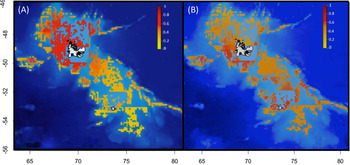
Targeting background records has been extensively tested, and several procedures have been developed to significantly improve the relevance of models (Fig. 5). Background records can be sampled within predefined areas (i.e. ‘discs’ or ‘buffers') close to presence records (Hengl et al. Reference Hengl, Sierdsema, Radovic´ and Dilo2009, Phillips et al. Reference Phillips, Dudík, Elith, Graham, Lehmann, Leathwick and Ferrier2009, Fourcade et al. Reference Fourcade, Engler, Rödder and Secondi2014, Bertrand et al. Reference Bertrand, Habasque, Hattab, Hintzen, Oliveros-Ramos and Gutiérrez2016), following the presence or absence of other species (Phillips et al. Reference Phillips, Dudík, Elith, Graham, Lehmann, Leathwick and Ferrier2009, Syfert et al. Reference Syfert, Smith and Coomes2013, Iturbide et al. Reference Iturbide, Bedia, Herrera, del Hierro, Pinto and Gutiérrez2015, Molloy et al. Reference Molloy, Davis, Dunlop and van Etten2017, Phillips et al. Reference Phillips, Reid, Thys, Harrod, Payne and Morgan2017, Ranc et al. Reference Ranc, Santini, Rondinini, Boitani, Poitevin, Angerbjörn and Maiorano2017), according to probabilities given by a kernel density estimator of the sampling frequency (Fourcade et al. Reference Fourcade, Engler, Rödder and Secondi2014, Jarnevich et al. Reference Jarnevich, Talbert, Morisette, Aldridge, Brown and Kumar2017, Guillaumot et al. Reference Guillaumot, Martin, Eléaume and Saucède2018a, Fabri-Ruiz et al. Reference Fabri-Ruiz, Danis, David and Saucède2019) or according to additive descriptors of accessibility and sampling effort (El-Gabbas & Dormann Reference El-Gabbas and Dormann2018). Once again, the selected method should be adapted to each case study and its efficiency tested prior to model interpretation (Støa et al. Reference Støa, Halvorsen, Mazzoni and Gusarov2018).
Comparison of predicted distribution probabilities (between 0 and 1) of the sea urchin Ctenocidaris nutrix on the Kerguelen Plateau: a. without compensating for sampling bias; b. with a kernel density estimator (KDE) correction. More background data are sampled in highly sampled areas. The spatial aggregation of presence-only records near the shoreline of the Kerguelen Islands strongly biases model predictions. The KDE correction was proven to be efficient at correcting for such a bias and provides more relevant predictions. From Guillaumot et al. (Reference Guillaumot, Martin, Eléaume and Saucède2018a).

A second method consists of filtering the available presence data to reduce the influence of the clustering of species records (Segurado et al. Reference Segurado, Araujo and Kunin2006, Kramer-Schadt et al. Reference Kramer-Schadt, Niedballa, Pilgrim, Schröder, Lindenborn and Reinfelder2013, Boria et al. Reference Boria, Olson, Goodman and Anderson2014). This is an efficient method compared to the background targeted sampling approach detailed above, but the remaining number of presence records after filtering should be sufficient to correctly determine species-occupied space (Kramer-Schadt et al. Reference Kramer-Schadt, Niedballa, Pilgrim, Schröder, Lindenborn and Reinfelder2013). Reliable information should also be available to characterize the bias in species occurrence data (Aiello-Lammens et al. Reference Aiello-Lammens, Boria, Radosavljevic, Vilela and Anderson2015, Sillero & Barbosa Reference Sillero and Barbosa2021). The filtering protocol requires meeting many prerequisites, but priority is given to keeping presence data independent and minimizing records clustering (D. Alagador, personal communication 2019).
Overall, if several methods are developed to correct for the effect of spatial aggregation on model outputs, it is recommended that one should interpret model projections performed for poorly sampled areas with great caution (Phillips et al. Reference Phillips, Dudík, Elith, Graham, Lehmann, Leathwick and Ferrier2009, Iturbide et al. Reference Iturbide, Bedia and Gutiérrez2018).
Model outputs
Taxonomic bias and population variability
SDMs are usually parameterized using all presence records available for a species and all environmental conditions prevailing in the species records (Elith & Leathwick Reference Elith and Leathwick2009). When modelling species distribution at a broad spatial scale, it is often assumed that all populations of a species have the same relationship to environmental conditions over the entire distribution area (Pierrat et al. Reference Pierrat, Saucède, Laffont, De Ridder, Festeau and David2012, Xavier et al. Reference Xavier, Raymond, Jones and Griffiths2016, Guillaumot et al. Reference Guillaumot, Fabri-Ruiz, Martin, Eléaume, Danis, Féral and Saucède2018b, Fabri-Ruiz et al. Reference Fabri-Ruiz, Danis, David and Saucède2019). However, occurrence datasets may include a set of populations with different phenotypic plasticities (Chevin et al. Reference Chevin, Lande and Mace2010), transgenerational adaptations (Dixon et al. Reference Dixon, Davies, Aglyamova, Meyer, Bay and Matz2015) or simply different habitat selection in the case of vagile species. Therefore, the modelled species can actually present different abilities to respond to environmental changes. In particular, physiological performances of populations are likely to vary in marine species with wide distribution ranges and high dispersal capabilities over long distances (Thatje Reference Thatje2012). This is particularly relevant with regards to future predictions that do not integrate inter-population variability in the potential acclimation of species, and this may lead models to alternatively over- or under-estimate the distribution of species-suitable environments (Cacciapaglia & van Woesik Reference Cacciapaglia and van Woesik2017, Thyrring et al. Reference Thyrring, Bundgaard and Sejr2017).
Phylogeographical studies have also regularly revealed the existence of cryptic species in the SO benthos, which show similar morphologies for distinct genotypes and potentially distinct ecological requirements and geographical distributions (Lozier et al. Reference Lozier, Aniello and Hickerson2009). Such studies often stress the need for taxonomic revisions (González-Wevar et al. Reference González-Wevar, Hüne, Rosenfeld, Nakano, Saucède, Spencer and Poulin2019, Ocaranza-Barrera et al. Reference Ocaranza-Barrera, González-Wevar, Guillemin, Rosenfeld and Mansilla2019, Moreau et al. Reference Moreau, Jossart, Danis, Eléaume, Christiansen and Guillaumot2021). SDMs can be generated based on a spatial subdivision of presence records according to the genetic structure of taxa, and in a second step, the different predictions can be merged together to the broader scale (Knowles et al. Reference Knowles, Carstens and Keat2007, Marcer et al. Reference Marcer, Méndez-Vigo, Alonso-Blanco and Picó2016, Cacciapaglia & van Woesik Reference Cacciapaglia and van Woesik2017, Ikeda et al. Reference Ikeda, Max, Allan, Lau, Shuster and Whitham2017, Roberts et al. Reference Roberts, Bahn, Ciuti, Boyce, Elith and Guillera-Arroita2017, Pardo-Gandarillas et al. Reference Pardo-Gandarillas, Ibáñez, Torres, Sanhueza, Fabres and Escobar-Dodero2018). However, defining the genetic structure of benthic species in the SO is a long-term endeavour that requires a constantly renewed sampling effort, considering the extent and complexity of the study area (Moreau et al. Reference Moreau, Saucède, Jossart, Agüera, Brayard and Danis2017, Fraser et al. Reference Fraser, Morrison, Hogg, Macaya, van Sebille and Ryan2018, Moore et al. Reference Moore, Carvajal, Rouse and Wilson2018). Waiting for taxonomic revisions and enhanced sampling efforts to best depict relationships between genetic units and environmental conditions (Vandersteen Reference Vandersteen2011) and combining SDMs with experimental data or mechanistic approaches can be alternatives for taking into account the possible physiological contrasts between populations (Kearney & Porter Reference Kearney and Porter2009, Buckley et al. Reference Buckley, Urban, Angilletta, Crozier, Rissler and Sears2010, Kearney et al. Reference Kearney, Wintle and Porter2010, Fordham et al. Reference Fordham, Mellin, Russell, Akçakaya, Bradshaw and Aiello-Lammens2013, Briscoe et al. Reference Briscoe, Kearney, Taylor and Wintle2016, Feng & Papes Reference Feng and Papeş2017, López-Farrán et al. Reference López-Farrán, Guillaumot, Vargas-Chacoff, Paschke, Dulière and Danis2021).
Definition of the projection area
The limitations in the current knowledge of species distribution also affect the quality of information available for estimating their potential distribution (Thuiller et al. Reference Thuiller, Vayreda, Pino, Sabate, Lavorel and Gracia2003). When the limits of species environmental ranges are not fully captured, this uncertainty can significantly impact the accuracy of SDM predictions (Hortal et al. Reference Hortal, Lobo and Jiménez-Valverde2007, Reference Hortal, Jiménez-Valverde, Gómez, Lobo and Baselga2008, Rocchini et al. Reference Rocchini, Hortal, Lengyel, Lobo, Jimenez-Valverde and Ricotta2011, Sánchez-Fernández et al. Reference Sánchez-Fernández, Lobo and Hernández-Manrique2011, Titeux et al. Reference Titeux, Maes, Van Daele, Onkelinx, Heikkinen and Romo2017, El-Gabbas & Dormann Reference El-Gabbas and Dormann2018). It reduces the applicability of models for predictive purposes (Thuiller et al. Reference Thuiller, Brotons, Araújo and Lavorel2004), induces model overfitting (Tsoar et al. Reference Tsoar, Allouche, Steinitz, Rotem and Kadmon2007, Barve et al. Reference Barve, Barve, Jiménez-Valverde, Lira-Noriega, Maher and Peterson2011, Guillaumot et al. Reference Guillaumot, Fabri-Ruiz, Martin, Eléaume, Danis, Féral and Saucède2018b) and can lead to overestimating the extent of suitable areas (Anderson & Raza Reference Anderson and Raza2010). This bias can be partly overcome by reducing the extent of the projection area to the known distribution of the available occurrence records (Anderson & Raza Reference Anderson and Raza2010) and by increasing knowledge regarding species ecology and physiology in order to identify the environmental conditions that are unsuitable for their survival or development (Byrne et al. Reference Byrne, Gall, Wolfe and Agüera2016).
Model extrapolation
Models are said to extrapolate when a portion of the predicted area includes environmental conditions that are outside the range of values for which the model was calibrated. Model extrapolation may occur when model predictions are transferred, either in space or time. When extrapolated, model predictions are in non-analogue conditions compared to the initial calibration conditions because calibration data may not encompass the entire environmental range of each of the predictors (Guillaumot et al. Reference Guillaumot, Moreau, Danis and Saucède2020b). The set of projected environmental conditions can otherwise still be within the range of conditions, but specific combinations of environmental descriptors may be new, also leading to extrapolation (Mesgaran et al. Reference Mesgaran, Cousens and Webber2014). In such conditions, predictions might be ecologically and statistically invalid and model interpretations inaccurate (Randin et al. Reference Randin, Dirnböck, Dullinger, Zimmermann, Zappa and Guisan2006, Williams & Jackson Reference Williams and Jackson2007, Williams et al. Reference Williams, Jackson and Kutzbach2007, Fitzpatrick & Hargrove Reference Fitzpatrick and Hargrove2009, Owens et al. Reference Owens, Campbell, Dornak, Saupe, Barve and Soberón2013).
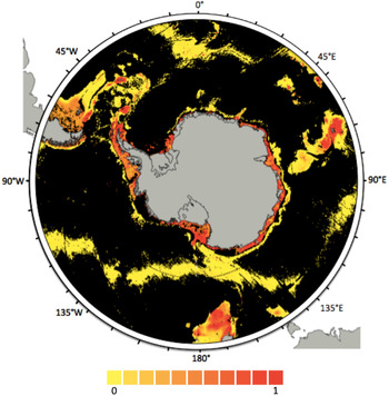
Among the different approaches, Elith et al. (Reference Elith, Kearney and Phillips2010) propose estimating and quantifying model extrapolation using the Multivariate Environmental Similarity Surface (MESS) index to identify the most influential descriptors that lead to extrapolation. Grid-cell pixels for which at least one environmental descriptor has a value outside the range of environmental values defined by presence-only records (calibration range) are considered to be extrapolations. In these cases, the MESS index gives negative values and the ensemble of pixels containing negative values defines the extrapolation area (Elith et al. Reference Elith, Kearney and Phillips2010, Guillaumot et al. Reference Guillaumot, Moreau, Danis and Saucède2020b). Most often, for SDMs performed at the scale of the SO, the number of records available to define the environmental space occupied by species is limiting and the resolution of environmental descriptors relatively low (see the ‘Quality of datasets’ section). As a consequence, SDM projections sometimes include wide extrapolation areas that may cover > 75% of the predicted regions (Fig. 6; Guillaumot et al. Reference Guillaumot, Moreau, Danis and Saucède2020b).
Extrapolation map of the species distribution model generated for the sea star Acodontaster hodgsoni, with all presence-only records available. Extrapolation corresponds here to the ensemble of environmental conditions that are outside of the boundaries of the calibration range. The extrapolation area is displayed in black and covers 78.6% of the entire projection area; coloured pixels (yellow-red colour palette) show distribution probabilities (included between 0 and 1). Extracted from Guillaumot et al. (Reference Guillaumot, Moreau, Danis and Saucède2020b).

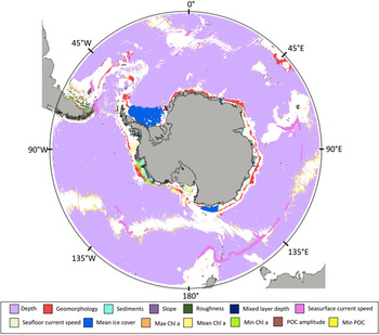
In addition to quantifying the overall extrapolation area (Fig. 6), it is possible to fine-tune the analysis and define which environmental descriptors and areas are concerned with extrapolation (Fig. 7; Owens et al. Reference Owens, Campbell, Dornak, Saupe, Barve and Soberón2013, https://CRAN.R-project.org/package=SDMPlay). Such information could be used to resample the environmental descriptors implemented in the model.
Extrapolation map of the species distribution model generated for the sea star Acodontaster hodgsoni indicating environmental descriptors responsible for extrapolation (black pixels of Fig. 6 are here coloured according to the descriptor responsible for extrapolation; i.e. for each pixel, the predictor in question lies outside the calibration range). In this case study, 14 environmental descriptors are responsible for extrapolation, with depth being the main contributor. White pixels correspond to areas where the model does not extrapolate (the corresponding model predictions are shown in Fig. 6). POC stands for ‘particulate organic carbon’ and Chl a is the concentration in chlorophyll a on the sea surface. Generated from https://cran.r-project.org/package=SDMPlay.

In any case, it has been recommended to provide information on model extrapolation and more generally to other concepts of uncertainties (species detection, errors, etc.), along with model predictions, because they are essential to accurate interpretation (Beale & Lennon Reference Beale and Lennon2012, Addison et al. Reference Addison, Rumpff, Bau, Carey, Chee and Jarrad2013, Guisan et al. Reference Guisan, Tingley, Baumgartner, Naujokaitis-Lewis, Sutcliffe and Tulloch2013).
Limiting model projections to ‘realistic’ depth ranges or some other environmental limiting factor based on a robust knowledge of species ecology (i.e. some expert-driven decision) was proven to be efficient at reducing extrapolation (Kearney & Porter Reference Kearney and Porter2009, Hare et al. Reference Hare, Wuenschel and Kimball2012, De Villiers et al. Reference De Villiers, Hattingh and Kriticos2013, Guillaumot et al. Reference Guillaumot, Moreau, Danis and Saucède2020b). Such a strategy is transitional until complementary samples and more comprehensive occurrence datasets are made available to better define the species-occupied space (Guillaumot et al. Reference Guillaumot, Moreau, Danis and Saucède2020b).
Model validation and accuracy of model predictions
Some common metrics for the evaluation of model predictions
Once models are generated, the accuracy of their predictions must be assessed in order to evaluate the validity of the models with regards to scientific issues to address, to compare different model outputs and to allow for the formulation of reliable interpretations (Zurell et al. Reference Zurell, Franklin, König, Bouchet, Dormann and Elith2020). Several metrics were developed in order to evaluate the performance of models (Fielding & Bell Reference Fielding and Bell1997, Allouche et al. Reference Allouche, Tsoar and Kadmon2006). Most of them are based on the calculation of an error matrix (or confusion matrix) that displays the proportion of presence and absence records that are correctly predicted by the model (Allouche et al. Reference Allouche, Tsoar and Kadmon2006).
In most biological studies focused on the SO benthos, absence records are usually unavailable and SDMs are generated based on a set of presence/background records (see the ‘Occurrence datasets’ section). As a consequence, the statistics that are commonly used for presence/absence datasets may not be appropriate for model evaluation (Wiley et al. Reference Wiley, McNyset, Peterson, Robins and Stewart2003, Phillips et al. Reference Phillips, Anderson and Schapire2006, Braunish et al. Reference Braunisch, Coppes, Arlettaz, Suchant, Schmid and Bollmann2013), such as the κ statistic (Allouche et al. Reference Allouche, Tsoar and Kadmon2006). In contrast, the area under the curve or area under the receiver operating curve (AUC) is one of the most used and appropriate metrics for measuring the performance of model predictions based on presence/background data (Hand Reference Hand2009). The AUC is an objective measure that remains stable with low-prevalence datasets (i.e. low frequency of occurrences with regards to the projection space) and is not sensitive to threshold effects (Manel et al. Reference Manel, Williams and Ormerod2001, Hand Reference Hand2009, van Proosdij et al. Reference Van Proosdij, Sosef, Wieringa and Raes2016). However, for presence/background models, specificity (the fraction of correctly predicted absences) might be overestimated when the number of background records is much higher than the number of presence-only records or when background and presences are associated with very different environmental values. This incidentally inflates AUC scores (Phillips et al. Reference Phillips, Anderson and Schapire2006, Raes & ter Steege Reference Raes and ter Steege2007, Lobo Reference Lobo2008, Jiménez-Valverde Reference Jiménez-Valverde2012) and invalidates the relevance of the AUC metrics (van Proosdij et al. Reference Van Proosdij, Sosef, Wieringa and Raes2016).
Even when properly employed, the AUC cannot be used to compare models when SDMs are generated for different species based on different environmental descriptors or projected on distinct regions because the values depend on the relative size of suitable areas and prevalence scores may contrast (see the ‘Correcting spatial biases’ section) (Wisz et al. Reference Wisz, Hijmans, Li, Peterson, Graham and Guisan2008, Anderson & Gonzalez Reference Anderson and Gonzalez2011). The AUC metrics must be used as a simple measure of the relative ranking of model predictions associated with a specific dataset (El-Gabbas & Dormann Reference El-Gabbas and Dormann2018). Overall, each statistic is characterized by specific advantages and potential biases, so that it is recommended that one uses several statistics for evaluating model predictions (Allouche et al. Reference Allouche, Tsoar and Kadmon2006).
The accuracy of model predictions can also be evaluated by testing the classification of independent test data, where the available occurrence dataset can be split into independent subsets to train or test the model (for a review, see Fielding & Bell Reference Fielding and Bell1997).
Cross-validation procedures
Cross-validation procedures are aimed at evaluating model predictions using a subset of presence or absence records retrieved from the initial dataset used for modelling in order to assess how well the test data match with the modelled predictions (Bahn & McGill Reference Bahn and McGill2013). When working with presence-only datasets, two subsets of presence records are used: one subset is used to train the model (the training group) and the second subset is used to test the model (the test group). Test data and training data must be spatially independent from each other (Hijmans Reference Hijmans2012, Bahn & McGill Reference Bahn and McGill2013). In most modelling exercises, standard cross-validation procedures are commonly used, in which the initial presence dataset is randomly split into a training and test subset. Frequently, as previously discussed, presence data are spatially aggregated in SO datasets and the necessary condition of independence between training and test data is seldom met, making the model accuracy evaluation overly optimistic (Telford & Birks Reference Telford and Birks2009, Hijmans Reference Hijmans2012, Radosavljevic & Anderson Reference Radosavljevic and Anderson2014). In contrast to random procedures, spatial cross-validation procedures improve the performance of the validation step by spatially segregating the training and test subsets, ensuring the spatial independence between data even when they are spatially aggregated in the initial datasets (Dhingra et al. Reference Dhingra, Artois, Robinson, Linard, Chaiban and Xenarios2016, Roberts et al. Reference Roberts, Bahn, Ciuti, Boyce, Elith and Guillera-Arroita2017, Guillaumot et al. Reference Guillaumot, Artois, Saucède, Demoustier, Moreau and Eléaume2019; see also http://cran.rapporter.net/web/packages/blockCV/vignettes/BlockCV_for_SDM.html).
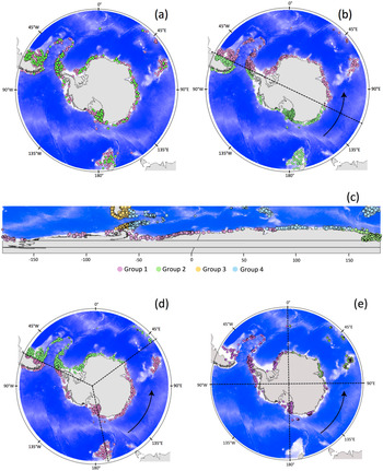
Several spatial cross-validation procedures have been proposed (Fig. 8), and the most appropriate one can be determined by comparing the different procedures in order to define the one that is most suitable for the study (Muscarella et al. Reference Muscarella, Galante, Soley-Guardia, Boria, Kass, Uriarte and Anderson2014, Radosavljevic & Anderson Reference Radosavljevic and Anderson2014, Guillaumot et al. Reference Guillaumot, Artois, Saucède, Demoustier, Moreau and Eléaume2019, Valavi et al. Reference Valavi, Elith, Lahoz-Monfort and Guillera-Arroita2019) depending on the spatial scale of the analysis, the number and spatial distribution of the presence data and the selected algorithm (and its associated complexity) used for modelling (El-Gabbas & Dormann Reference El-Gabbas and Dormann2018, Hao et al. Reference Hao, Elith, Lahoz-Monfort and Guillera-Arroita2020).
Different cross-validation procedures based on the study of the sea star Odontaster validus, showing presence-only records and a random set of 1,000 background data selected according to a kernel density estimation weighting scheme from the dataset of Griffiths et al. (Reference Griffiths, Van de Putte, Danis, De Broyer, Koubbi, Griffiths, Raymond and Udekem d'Acoz2014) on sampling effort of the Southern Ocean benthos. Data are split into training (pink) and test (green) subsets. The blue background corresponds to bathymetry and grey areas to emerged lands. a. Random cross-validation procedure, with a random split into 75% training and 25% test data. b. ‘Twofold CLOCK’ clustering by random spatial partition of the dataset into two groups (one training and one test). c. ‘BLOCK’ splitting, generated according to median latitudinal and longitudinal values (Muscarella et al. Reference Muscarella, Galante, Soley-Guardia, Boria, Kass, Uriarte and Anderson2014). After the generation of four groups (corresponding to the four colours), one group is randomly defined as the test subset and the other three groups as the training subsets. A different system of projection was used to represent this map in order to highlight the latitudinal and longitudinal definition of the transects. d. ‘Threefold CLOCK’ clustering by random spatial partition of the dataset into three groups (two training and one test). e. ‘Fourfold CLOCK’ clustering by random spatial partition of the dataset into four groups (three training and one test). Extracted from Guillaumot et al. (Reference Guillaumot, Artois, Saucède, Demoustier, Moreau and Eléaume2019).

Conclusions and future prospects
This review summarizes some points and issues to be considered during SDM construction for modelling the distribution of SO species (Fig. 1). It shows that accurate and efficient SDMs can be produced for SO species when considering potential common biases and issues and correcting for their side effects. Proposed corrections must be adjusted to each case study: no consensus method nor implementation procedure always perform best - each case study requires proper analyses in order to generate the most relevant and accurate predictions. This means that, for each model, several procedures to implement the model should be tested in order to select the most suitable one, ideally giving priority to the availability of independent datasets for evaluating the models. We showed that SDMs perform best when the species-occupied space is accurately described, using extensive occurrence datasets with both presence and absence records, and when data are checked for positioning and georeferencing errors. A good knowledge of species’ ecology, life history traits and populational variations within the overall species distribution and environmental range help to improve model quality (Fois et al. Reference Fois, Cuena-Lombraña, Fenu and Bacchetta2018). The compilation, examination and preparation of datasets prior to modelling are essential steps in generating efficient models. Estimating and communicating the uncertainties associated with model predictions are also important tasks to be highlighted. This process may include a ‘simple’ interpretation of the ecological relevance of SDM outputs by experts (Merow et al. Reference Merow, Wilson and Jetz2017) for the mapping of model extrapolations, as illustrated here. Model uncertainties are part of model outputs and should not be omitted (Guisan et al. Reference Guisan, Tingley, Baumgartner, Naujokaitis-Lewis, Sutcliffe and Tulloch2013, Grimm et al. Reference Grimm, Augusiak, Focks, Frank, Gabsi and Johnston2014, Grimm & Berger Reference Grimm and Berger2016).
Remaining challenges for constructing relevant SDMs for SO studies include more efforts regarding data collection outside of the main sampling hotspots and filling in knowledge gaps in SO species taxonomy. Some methodological perspectives, developed in other regions, address the integration of physiological information into SDMs. This facilitates the understanding of species environmental preferences and helps one to better estimate the niches of species (Kearney & Porter Reference Kearney and Porter2009, Talluto et al. Reference Talluto, Boulangeat, Ameztegui, Aubin, Berteaux and Butler2016, Mathewson et al. Reference Mathewson, Moyer-Horner, Beever, Briscoe, Kearney, Yahn and Porter2017, Rodríguez et al. Reference Rodríguez, García, Carreño and Martínez2019, Gamliel et al. Reference Gamliel, Buba, Guy-Haim, Garval, Willette, Rilov and Belmaker2020). Such studies have recently been developed for SO benthic species: in López-Farrán et al. (Reference López-Farrán, Guillaumot, Vargas-Chacoff, Paschke, Dulière and Danis2021), the combination of physiological experimental results and SDM projections allowed for the assessment of the invasive potential of the Patagonian crab Halicarcinus planatus (Fabricius, 1775) on Antarctic coasts, as was similarly done in Byrne et al. (Reference Byrne, Gall, Wolfe and Agüera2016) for the Arctic sea star Asterias amurensis (Lutken, 1871). Hybrid modelling approaches constitute another exciting approach, where information from both SDMs and physiological models are fully integrated, using the physiological information as a prior to inform the SDM (Gamliel et al. Reference Gamliel, Buba, Guy-Haim, Garval, Willette, Rilov and Belmaker2020). Recently applied to an endemic sea urchin of the Kerguelen Plateau (C. Guillaumot et al., unpublished data 2021), the method allows for more precise prediction of the effects of seasonal variations on species habitat suitability.
Other interesting methodological approaches include the consideration of biotic interaction information, dispersal capacity estimates or population dynamics in complement to SDM predictions in order to generalize the understanding of the main drivers of species distribution (Pellissier et al. Reference Pellissier, Anne Bråthen, Pottier, Randin, Vittoz and Dubuis2010, Meier et al. Reference Meier, Edwards, Kienast, Dobbertin and Zimmermann2011, Pagel & Schurr Reference Pagel and Schurr2012, Conlisk et al. Reference Conlisk, Syphard, Franklin, Flint, Flint and Regan2013, Pellissier et al. Reference Pellissier, Rohr, Ndiribe, Pradervand, Salamin, Guisan and Wisz2013, Leach et al. Reference Leach, Montgomery and Reid2016, Anderson Reference Anderson2017). These, however, necessitate a deep knowledge of the species ecology and of the surrounding environment, suggesting that their first applications should be expected in local- or regional-scale studies.
A final take-home message is that model outputs should be interpreted carefully and model predictions always considered with a critical eye. Models are simple representations of complex systems and should be used to complement other approaches in order to support conservation strategies or to address fundamental research objectives (Porfirio et al. Reference Porfirio, Harris, Lefroy, Hugh, Gould and Lee2014, Kampichler & Sierdsema et al. Reference Kampichler and Sierdsema2018).
Financial support
This work was supported by ‘Fonds pour la formation à la Recherche dans l'Industrie et l'Agriculture’ (FRIA) and ‘Bourse fondation de la mer’ grants to C. Guillaumot. This is contribution no. 47 to the vERSO project (www.versoproject.be), funded by the Belgian Science Policy Office (BELSPO, contract n°BR/132/A1/vERSO). Research was also financed by the ‘Refugia and Ecosystem Tolerance in the Southern Ocean’ project (RECTO; BR/154/A1/RECTO) funded by the Belgian Science Policy Office (BELSPO), this study being contribution number 24.