1 Introduction
The determination of laminar to turbulent transition in supersonic flows is crucial for the aero- and aerothermodynamic design of re-entry vehicles (Pate Reference Pate1977; Khan & Reshotko Reference Khan, Reshotko, Eppler and Fasel1980). The predicted heat flux, which in turbulent compared to laminar boundary layers can be higher by more than just one order of magnitude, is an essential design parameter (Wurster Reference Wurster1981; Lin, Grabowsky & Yelmgren Reference Lin, Grabowsky and Yelmgren1984; Bouslog et al. Reference Bouslog, An, Hartmann and Derry1991). Since experimental wind tunnel data of boundary layer transition are known to be affected by tunnel noise (Reshotko Reference Reshotko1994; Fedorov Reference Fedorov2003, Reference Fedorov2011; Ma & Zhong Reference Ma and Zhong2003a ,Reference Ma and Zhong b , Reference Ma and Zhong2005; Zhong & Wang Reference Zhong and Wang2012; Fedorov et al. Reference Fedorov, Ryzhov, Soudakov and Utyuzhnikov2013), i.e. it strongly influences the region of transition (Schneider Reference Schneider2001, Reference Schneider2008a ,Reference Schneider b ), it is necessary to know the noise inherent to the test facility to properly evaluate and interpret the experimental results. Furthermore, the knowledge of the wind tunnel noise is essential to numerically compute the receptivity phenomenon for the specific noise of the wind tunnel and thus, to improve the similarity between experiment and simulation.
To understand the general term tunnel noise, the work of Kovasznay (Reference Kovasznay1953) and Morkovin (Reference Morkovin1956) on fluctuations in compressible flows is essential. Kovasznay found three coexisting modes, i.e. acoustic, entropy and vorticity, obeying separate linear differential equations, if the perturbations are small, and exhibiting moderate interaction at increasing strength. While the vorticity and entropy mode behave as a ‘frozen pattern’ and convect with the fluid, the acoustic mode obeys a wave equation and propagates with the speed of sound. Altogether, the three modes superimpose continuously in the frequency domain inhering various spatial distributions and form the tunnel noise (Grossir, Masutti & Chazot Reference Grossir, Masutti and Chazot2015).
In the past, to measure tunnel noise, hot-wires and Pitot probes have been used as intrusive measuring techniques. The hot-wire is sensitive to total temperature and mass flow, which are both conserved across the shock wave. However, these are not the variables of the fluctuation modes derived by Kovasznay (Reference Kovasznay1953). Therefore, a subsequent analysis, i.e. modal analysis or modal decomposition, is employed to yield the fluctuation modes. Logan (Reference Logan1988) states that the two hot-wire variables cannot be decomposed into the three fluctuation mode variables without further information, e.g. assumptions, equations or measurements.
Pitot probes measure the postshock total pressure
 $p_{t}$
which is related to the preshock static pressure
 $p_{\infty }$
and the Mach number
 $Ma_{\infty }$
by the Rayleigh Pitot tube formula
 $p_{t}=f(p_{\infty },Ma_{\infty })$
. Recently, Chaudhry & Candler linearized the Rayleigh Pitot tube formula
 $$\begin{eqnarray}\text{d}p_{t}=\frac{\unicode[STIX]{x2202}f}{\unicode[STIX]{x2202}p_{\infty }}\,\text{d}p_{\infty }+\frac{\unicode[STIX]{x2202}f}{\unicode[STIX]{x2202}Ma_{\infty }}\left(\frac{\unicode[STIX]{x2202}Ma_{\infty }}{\unicode[STIX]{x2202}u_{\infty }}\,\text{d}u_{\infty }+\frac{\unicode[STIX]{x2202}Ma_{\infty }}{\unicode[STIX]{x2202}T_{\infty }}\,\text{d}T_{\infty }\right)\end{eqnarray}$$
and showed that the relation between postshock total pressure fluctuations and preshock fluctuations of state and flow is not unique since acoustic (
 $\text{d}p_{\infty }$
, static temperature
 $\text{d}T_{\infty }$
, velocity
 $\text{d}u_{\infty }$
), entropy (
 $\text{d}T_{\infty }$
) and vorticity (
 $\text{d}u_{\infty }$
) modes generate postshock total pressure fluctuations (Chaudhry & Candler Reference Chaudhry and Candler2016). In general, the interaction of any single mode type of the tunnel noise and the shock wave causes a modulation of the perturbations, i.e. the single mode type is transmitted and the remaining mode types are generated (McKenzie & Westphal Reference McKenzie and Westphal1968; Anyiwo & Bushnell Reference Anyiwo and Bushnell1982; Schilden et al.
Reference Schilden, Schröder, Ali, Wu, Schreyer and Radespiel2016). Furthermore, Chaudhry & Candler proved (1.1) to be invalid beyond the low frequency limit using numerical simulations. They investigated the pressure response of a cylindrical Pitot probe under various supersonic flow configurations to incident plane continuous acoustic and entropy waves. For any incident disturbance type, at certain frequencies, oscillating acoustic waves in the subsonic region between shock wave and Pitot probe lead, against Morkovin’s (Reference Morkovin1960) hypothesis of rather scattered than focused acoustic waves downstream of the shock wave, to significant positive interference. This positive interference was also found experimentally by Ali et al. (Reference Ali, Zárate Cárdenas, Radespiel, Schilden and Schröder2018). Note that constructive interference was also found equipping the probe with a heat flux transducer. Since the frequency response of a Pitot probe deviates from the analytic low frequency limit due to resonance, it is necessary to obtain transfer functions that relate the postshock measured total pressure fluctuations to the fluctuation modes. Nonetheless, as for the hot-wire data, it is evident from (1.1) that further information for a modal decomposition is needed to gain a unique relation between Pitot probe data and the three fluctuation modes.
In the following, the development of hot-wire and Pitot probe modal analysis is briefly described and the significance of this work is discussed. In the scope of the derivation of the three disturbance modes, Kovasznay also developed the ‘fluctuation diagram’ to visualize hot-wire data (Kovasznay Reference Kovasznay1953). Including additional assumptions that can be deduced from the fluctuation diagram itself, it can be used to decompose the hot-wire data. Laufer (Reference Laufer1961) extended the method of Kovasznay for measuring normalized root-mean-square (nRMS) pressure fluctuations in acoustic dominated tunnels. Later, Logan proposed a new hot-wire modal analysis by considering separate static pressure fluctuation measurements using non-intrusive laser-induced fluorescence to decrease the number of assumptions for the modal analysis (Logan Reference Logan1988). Since non-intrusive optical measurement techniques are expensive and demand optical access, Masutti et al. (Reference Masutti, Spinosa, Chazot and Carbonaro2012), Wu, Zamre & Radespiel (Reference Wu, Zamre and Radespiel2015) and Schilden et al. (Reference Schilden, Schröder, Ali, Wu, Schreyer and Radespiel2016) apply the modal analysis method of Logan using an additional intrusive Pitot probe and neglect the aforementioned effect of free stream vorticity and entropy mode induced pressure fluctuations. Schilden et al. (Reference Schilden, Schröder, Ali, Wu, Schreyer and Radespiel2016) subdivided the hot-wire modal analysis in the frequency domain to analyse the frequency dependence of the fluctuation mode composition of tunnel noise. Furthermore, to overcome the frequency limitations of the hot-wire system, a new modal analysis approach was presented. Neglecting the weak vorticity mode, a cone probe equipped with pressure and heat flux transducers in the lateral surface was applied in the following decomposition
 $$\begin{eqnarray}\boldsymbol{F}_{w}=\unicode[STIX]{x1D64E}\boldsymbol{F}_{\infty }.\end{eqnarray}$$
In (1.2),
 $\boldsymbol{F}_{w}$
contains bandpass filtered measured heat flux and pressure fluctuations. They are related to the free stream fluctuation modes in that frequency range
 $\boldsymbol{F}_{\infty }$
via the transfer matrix
 $\unicode[STIX]{x1D64E}$
. The entries of the transfer matrix are determined by direct numerical simulation (DNS) for representative frequencies. Since the acoustic and entropy mode originate from different sources and obey different dispersion relations, they can be assumed to be uncorrelated (Laderman & Demetriades Reference Laderman and Demetriades1974). Therefore, the type of (1.2) also holds for nRMS values. It was shown that the modal analysis suffered from the heat flux transducer being located in the lateral surface of the cone. The boundary layer shields the transducer from postshock entropy waves whose contribution to the heat flux is essential for the proposed modal decomposition method. The decomposition using the inverse of the transfer matrix
 $\unicode[STIX]{x1D64E}$
proved to be too sensitive to input errors due to its high condition number. Still, using the measured heat flux and pressure fluctuations in combination with the numerically determined transfer functions of the acoustic mode separately, the acoustic noise level could be reconstructed up to 200 kHz. It was concluded that locating the transducers in the stagnation point of a probe would reduce the shielding towards postshock entropy waves.
In this study, the properties of stagnation point probes for the newly developed modal decomposition method following (1.2) are investigated by DNS. Pressure and heat flux responses to various fluctuation mode input functions are analysed to investigate the perception of postshock waves by the probe. By analysing the pressure and heat flux response to pulses of incident disturbances, a model equation for the perception of postshock waves by a stagnation point probe (SPP) is formulated to evaluate the importance of certain postshock waves and their contribution to pressure and heat flux fluctuations for the application of SPPs in the modal decomposition method (1.2). The important transfer functions are analysed separately by methods of control theory and the findings are compared to the frequency response to continuous incident disturbances.
The paper is organized as follows. First, the SPP of this investigation are presented and the flow conditions are outlined. In § 2, the numerical method and computational set-up of the simulations are presented. Then, the results of the manifold investigation are discussed. Finally, the essential findings are summarized and some conclusions are drawn.
2 Numerical method
2.1 Governing equations
The numerical simulations are based on the non-dimensionalized Navier–Stokes equations.
 $$\begin{eqnarray}\int _{V}\frac{\unicode[STIX]{x2202}\boldsymbol{Q}}{\unicode[STIX]{x2202}t}\,\text{d}V+\oint _{A}\overline{\boldsymbol{H}}\boldsymbol{\cdot }\boldsymbol{n}\,\text{d}A=\mathbf{0}.\end{eqnarray}$$
The quantity
 $\boldsymbol{Q}=[\unicode[STIX]{x1D70C},\unicode[STIX]{x1D70C}\boldsymbol{u}^{\text{T}},\unicode[STIX]{x1D70C}E]^{\text{T}}$
is the vector of the conservative variables with the density
 $\unicode[STIX]{x1D70C}$
, velocity vector
 $\boldsymbol{u}$
and the total specific energy
 $E=e+\boldsymbol{u}^{2}/2$
containing the specific energy
 $e$
. The flux vector
 $\overline{\boldsymbol{H}}$
can be decomposed into an inviscid
 $\overline{\boldsymbol{H}}^{i}$
and a viscous part
 $\overline{\boldsymbol{H}}^{v}$
 $$\begin{eqnarray}\overline{\boldsymbol{H}}=\overline{\boldsymbol{H}}^{i}+\overline{\boldsymbol{H}}^{v}=\left(\begin{array}{@{}c@{}}\unicode[STIX]{x1D70C}\boldsymbol{ u}^{\text{T}}\\ \unicode[STIX]{x1D70C}\boldsymbol{u}\boldsymbol{u}+\overline{\boldsymbol{I}}p\\ \boldsymbol{u}^{\text{T}}(\unicode[STIX]{x1D70C}E+p)\end{array}\right)+\frac{1}{Re_{0}}\left(\begin{array}{@{}c@{}}\mathbf{0}^{\text{T}}\\ \overline{\unicode[STIX]{x1D749}}\\ (\overline{\unicode[STIX]{x1D749}}\boldsymbol{u}+\boldsymbol{q})^{\text{T}}\end{array}\right).\end{eqnarray}$$
The Reynolds number is computed using the fluid properties at rest
 $Re_{0}=\unicode[STIX]{x1D70C}_{0}a_{0}l_{ref}/\unicode[STIX]{x1D702}_{0}$
, where
 $a$
denotes the speed of sound and
 $l_{ref}$
is the characteristic length. The dynamic viscosity
 $\unicode[STIX]{x1D702}$
is calculated using Sutherland’s law. Furthermore, the volume viscosity is assumed to be zero such that the stress tensor for a Newtonian fluid
 $\overline{\unicode[STIX]{x1D749}}$
can be written
 $$\begin{eqnarray}\overline{\unicode[STIX]{x1D749}}={\textstyle \frac{2}{3}}\unicode[STIX]{x1D702}(\unicode[STIX]{x1D735}\boldsymbol{\cdot }\boldsymbol{u})\overline{\boldsymbol{I}}-2\unicode[STIX]{x1D702}(\unicode[STIX]{x1D735}\boldsymbol{u}+(\unicode[STIX]{x1D735}\boldsymbol{u})^{\text{T}}).\end{eqnarray}$$
The vector of heat conduction
 $\boldsymbol{q}$
is formulated according to Fourier’s law
 $$\begin{eqnarray}\boldsymbol{q}=-\frac{\unicode[STIX]{x1D706}}{Pr(\unicode[STIX]{x1D6FE}-1)}\unicode[STIX]{x1D735}T\end{eqnarray}$$
using the gradient of the static temperature
 $\unicode[STIX]{x1D735}T$
, the thermal conductivity
 $\unicode[STIX]{x1D706}$
, the ratio of specific heats
 $\unicode[STIX]{x1D6FE}$
and the Prandtl number
 $Pr=\unicode[STIX]{x1D702}_{\infty }c_{p}/\unicode[STIX]{x1D706}_{\infty }$
, where
 $c_{p}$
is the specific heat at constant pressure.
The values for
 $\unicode[STIX]{x1D6FE}$
and
 $Pr$
at air flow are
 $\unicode[STIX]{x1D6FE}=1.4$
and
 $Pr=0.72$
. The system of equations is closed by the equation of state for an ideal gas
 $$\begin{eqnarray}e=\frac{p}{\unicode[STIX]{x1D70C}(\unicode[STIX]{x1D6FE}-1)}.\end{eqnarray}$$
2.2 Spatial and temporal approximation
The domain is discretized by an unstructured Cartesian grid and the governing equations are integrated using a finite-volume method (Hartmann, Meinke & Schröder Reference Hartmann, Meinke and Schröder2008; Schneiders et al.
Reference Schneiders, Hartmann, Meinke and Schröder2013; Lintermann et al.
Reference Lintermann, Schlimpert, Grimmen, Günther, Meinke and Schröder2014). For the spatial discretization an advection upstream splitting method (AUSM) is used. In this method, the advection Mach number on the cell surface is the mean of the extrapolated Mach numbers from the adjacent cells
 $Ma_{1/2}=0.5(Ma_{L}+Ma_{R})$
. The same formulation holds for the pressure on the cell surface. The cell centre gradients are computed using a second-order accurate least-squares reconstruction scheme (Hartmann et al.
Reference Hartmann, Meinke and Schröder2008). Shock capturing is achieved by adding additional numerical dissipation at the shock position. Furthermore, small cut cells are treated using an interpolation and flux-redistribution scheme developed by Schneiders et al. (Reference Schneiders, Hartmann, Meinke and Schröder2013). The temporal integration is based on a 5-stage second-order accurate Runge–Kutta scheme.
3 Computational set-up
For this investigation, we choose an operating point of the Hypersonic Ludwieg Tube Braunschweig at a Mach number of
 $Ma=5.9$
, a unit Reynolds number of
 $Re_{u}=6.25\times 10^{6}~\text{m}^{-1}$
and a total temperature of
 $T_{0}=470~\text{K}$
(Ali et al.
Reference Ali, Zárate Cárdenas, Radespiel, Schilden and Schröder2018). The flow is assumed to be laminar since the tunnel has a conventional nRMS fluctuation level of Pitot pressure between 1 and 1.6 % (Heitmann et al.
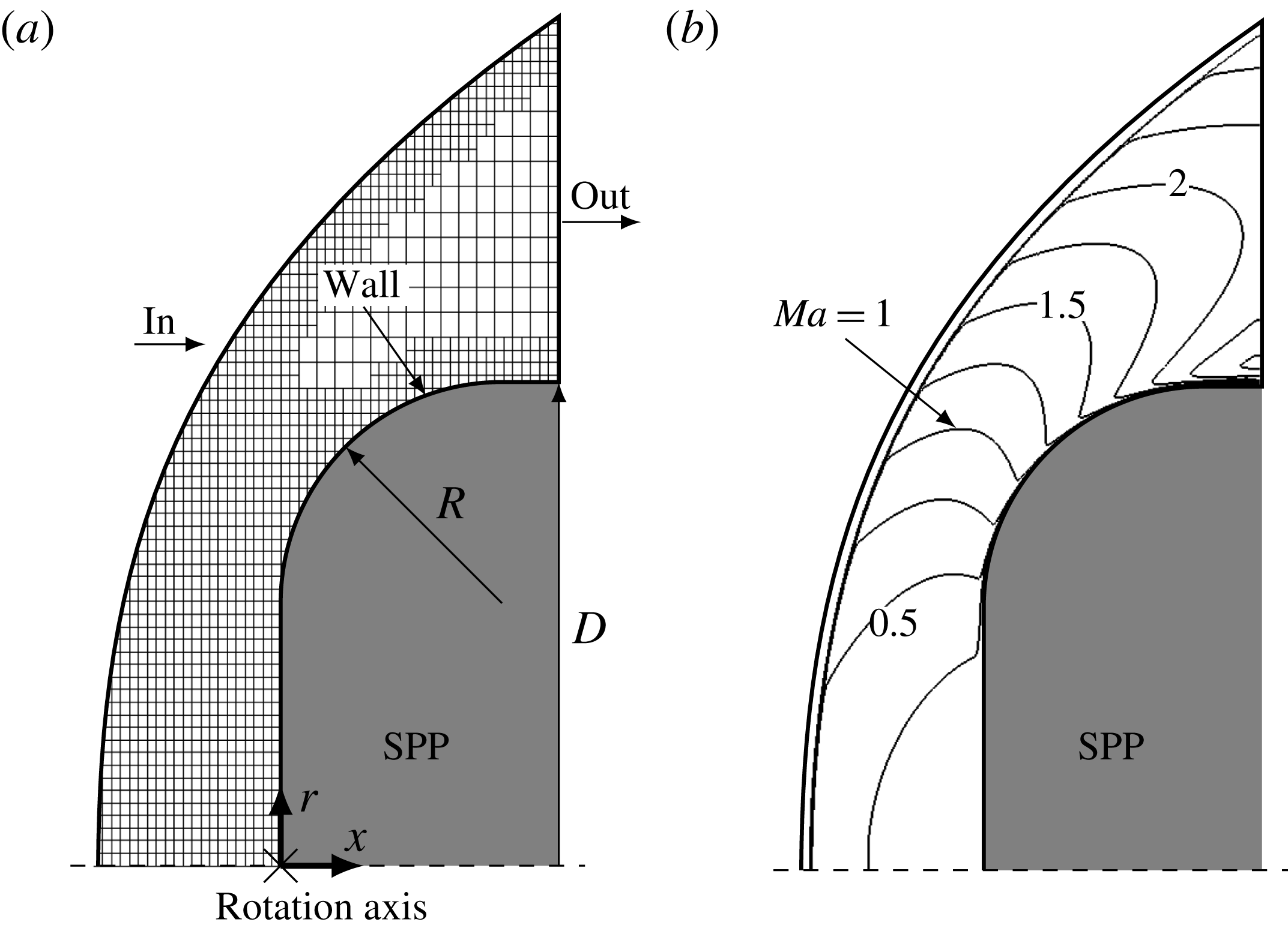
Reference Heitmann, Rödiger, Kähler, Knauss, Radespiel and Krämer2008). All perturbations in the free stream are assumed to be small enough to obey the linearized Euler equations, i.e. nonlinear interaction between acoustic and entropy modes does not occur. The stagnation point probes investigated in this study are schematically shown in figure 1(a). The geometry is identical to the ‘rounded’ configuration from Ali et al. (Reference Ali, Zárate Cárdenas, Radespiel, Schilden and Schröder2018). The probe is shaped like a cylinder and the axis of rotation is aligned with the flow. The transducer is mounted on the axis of rotation facing the flow, i.e. the sensitive transducer area coincides with the stagnation point. The cylinder edge on the transducer side is rounded. In general intrusive probes are designed to be as small as possible. Since the heat flux gauge is significantly larger than the pressure gauge, two similar probes of different size were manufactured. The smaller pressure probe is equipped with a PCB M12A32 sensor and has a diameter of
 $D=8~\text{mm}$
(Heitmann et al.
Reference Heitmann, Rödiger, Kähler, Knauss, Radespiel and Krämer2008). The larger heat flux probe contains an atomic layer thermopile sensor and the diameter is
 $D=17.5~\text{mm}$
(Knauss et al.
Reference Knauss, Roediger, Bountin, Smorodsky, Maslov and Srulijes2009; Kegerise & Rufer Reference Kegerise and Rufer2016). The ratio of probe diameter to the radius of the rounded edge is
 $D/R=4.375$
. It goes without saying that the Reynolds numbers based on the diameter of the probe must be different. The Reynolds numbers of the smaller pressure probe and larger heat flux probe are
 $Re_{D}=50\,000$
and
 $Re_{D}=109\,375$
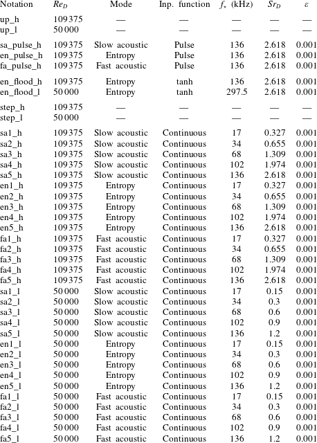
. The flow conditions are summarized in table 1.
Computational set-up and unperturbed flow field: (a) schematic of the SPP and boundary conditions of the DNS: supersonic inflow ‘in’, supersonic outflow ‘out’, solid isothermal no-slip wall ‘wall’, the cross ‘
 $\times$
’ denotes the sensor position at
 $x=0$
; (b) lines of constant Mach number downstream of the shock wave from case up_h,
 $\unicode[STIX]{x0394}Ma=0.25$
between the isolines.

Since the flow is axisymmetric, a periodic boundary condition formulation for Cartesian meshes by Pogorelov, Meinke & Schröder (Reference Pogorelov, Meinke and Schröder2015) is used to reduce the circumferential extent of the computational domain to a small finite segment of the three-dimensional domain. A schematic of the computational set-up is depicted in figure 1(a). On the upstream boundary ‘in’ supersonic Dirichlet conditions are prescribed for all variables. This boundary is located just upstream of the detached shock wave whose location is determined in a former simulation. On the outflow boundary ‘out’ supersonic outflow von Neumann conditions for all variables are applied. The SPP wall is modelled as a no-slip isothermal wall with a wall temperature of 295 K. The isothermal condition is justified by the short runtime of the wind tunnel of about 80 ms (Schilden et al. Reference Schilden, Schröder, Ali, Wu, Schreyer and Radespiel2016). Figure 1(a) indicates the grid used throughout the investigation. The unstructured grid is uniform between the shock wave and the SPP wall but is coarsened towards the outflow boundary. The grids in this study have 320 and 830 cells between the shock wave and the SPP along the rotation axis. The finer mesh is used for the high Reynolds number flows.
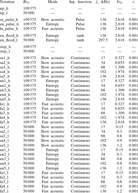
Flow parameters for the receptivity investigation: Reynolds number
 $Re_{D}=\unicode[STIX]{x1D70C}_{\infty }u_{\infty }D/\unicode[STIX]{x1D702}_{\infty }$
, frequency
 $f_{\star }$
, Strouhal number
 $Sr_{D}=D\unicode[STIX]{x1D714}/2\unicode[STIX]{x03C0}u_{\infty }$
, relative amplitude
 $\unicode[STIX]{x1D700}$
, the total temperature is always
 $T_{0,\star }=470~\text{K}$
, the wall surface is always
 $T_{w,\star }=295~\text{K}$
. The notation ‘up’ stands for unperturbed simulations; ‘sa’ defines a slow acoustic wave, ‘en’ an entropy wave, and ‘fa’ a fast acoustic wave, the numbers increase with increasing Strouhal number; ‘pulse’ stands for an incident pulse and ‘flood’ for a flooding of a certain mode; ‘step’ denotes simulations restarted with a slightly altered Reynolds number; ‘l’ stands for the lower Reynolds number and ‘h’ for the higher Reynolds number.
At the inlet, acoustic and entropy waves can be imposed. For an acoustic wave the pressure fluctuation
 $p^{\prime }$
is prescribed by
 $$\begin{eqnarray}p^{\prime }=\unicode[STIX]{x1D700}p_{\infty }\text{e}^{\text{i}(\boldsymbol{k}\boldsymbol{\cdot }\boldsymbol{x}-\unicode[STIX]{x1D714}t)}.\end{eqnarray}$$
The quantity
 $\boldsymbol{k}$
is the wave vector,
 $\unicode[STIX]{x1D714}$
the angular frequency and the quantity
 $\unicode[STIX]{x1D700}p_{\infty }$
denotes the pressure amplitude. The fluctuating density
 $\unicode[STIX]{x1D70C}^{\prime }$
and streamwise velocity
 $u^{\prime }$
follow from the one-dimensional linearized Euler equations for a fast (
 $+$
) and slow (
 $-$
) acoustic wave
 $$\begin{eqnarray}\left(\begin{array}{@{}c@{}}\unicode[STIX]{x1D70C}^{\prime }\\ u^{\prime }\end{array}\right)=\left(\begin{array}{@{}c@{}}{\displaystyle \frac{1}{a_{\infty }^{2}}}\\ {\displaystyle \frac{\pm 1}{\unicode[STIX]{x1D70C}_{\infty }a_{\infty }}}\end{array}\right)p^{\prime },\end{eqnarray}$$
where the subscript
 $\infty$
denotes quantities at free stream condition. The angular frequency is prescribed via the Strouhal number
 $$\begin{eqnarray}Sr=\frac{l_{ref}\unicode[STIX]{x1D714}}{2\unicode[STIX]{x03C0}u_{\infty }}.\end{eqnarray}$$
The wave vector and the angular frequency are related by the dispersion relation of acoustic waves
 $$\begin{eqnarray}\unicode[STIX]{x1D714}-\boldsymbol{u}_{\infty }\boldsymbol{\cdot }\boldsymbol{k}=\pm ka_{\infty },\end{eqnarray}$$
where
 $k$
is the magnitude of the wave vector. For an entropy wave, only the perturbed density
 $\unicode[STIX]{x1D70C}^{\prime }$
 $$\begin{eqnarray}\unicode[STIX]{x1D70C}^{\prime }=\unicode[STIX]{x1D700}\unicode[STIX]{x1D70C}_{\infty }\text{e}^{\text{i}(\boldsymbol{k}\boldsymbol{\cdot }\boldsymbol{x}-\unicode[STIX]{x1D714}t)},\end{eqnarray}$$
with an amplitude of
 $\unicode[STIX]{x1D700}\unicode[STIX]{x1D70C}_{\infty }$
is to be considered. The dispersion relation for the entropy wave reads
 $$\begin{eqnarray}\unicode[STIX]{x1D714}-\boldsymbol{u}_{\infty }\boldsymbol{\cdot }\boldsymbol{k}=0.\end{eqnarray}$$
4 Results
In this section, the results are discussed. The flow around an SPP at two Reynolds numbers is investigated. The response of the heat flux and pressure at the stagnation point to different disturbance modes and input functions is analysed. In table 1 all configurations are summarized in the order of the proximate discussion. In the figures of the analysis, most of the results will be presented using SI units. In the following, dimensional quantities are denoted by a subscript
 $\star$
. The discussion of the results is subdivided into five parts. First, the unperturbed flow field around the SPP at two Reynolds numbers and
 $Ma=5.9$
is presented in § 4.1. Then, the resonant behaviour is analysed by evaluating the SPP response to single pulses of incident acoustic and entropy mode disturbances in § 4.2. Based on the previous findings, a model equation for pressure and heat flux fluctuations is derived and discussed in § 4.3. In § 4.4, the step response of the SPP is investigated to gain the dynamic behaviour of the stagnation point heat flux. Finally, the frequency response of the SPP to continuous perturbations is analysed in § 4.5.
4.1 Unperturbed flow
The velocity field around the SPP, in general a blunt body, in supersonic and hypersonic flows is characterized by the detached bow shock and the large subsonic region downstream of the shock wave. In figure 1(b) Mach number contours from case up_h (unperturbed, high Reynolds number) are shown. Close to the inflow they all collapse and show the location of the shock wave. The flow in the subsonic region downstream of the bow shock is accelerated to supersonic speed half-way along the rounded edge. It is completely contained in the uniformly refined part of the grid. At the outflow downstream of the shock wave Mach numbers of approximately 2.5 are reached. The numerically determined heat flux
 $\bar{q}$
at the stagnation point for both Reynolds numbers is tabulated in table 2. It is higher for the lower Reynolds number case up_l (unperturbed, low Reynolds number). For validation purposes the stagnation point heat flux of the unperturbed flow is compared to corresponding experimental and numerical data from Ali et al. (Reference Ali, Zárate Cárdenas, Radespiel, Schilden and Schröder2018). The numerical value for case up_l is
 $\bar{q}_{\star }=71\,000~\text{W}~\text{m}^{-2}$
and the experimental comparative value for case up_h is
 $\bar{q}_{\star }=56\,000~\text{W}~\text{m}^{-2}$
. The good agreement of the simulations for up_l is evident and also the comparison with the experimental data for case up_h is convincing since the heat flux sensor has a large mean heat flux deviation of 20 % (Kegerise & Rufer Reference Kegerise and Rufer2016). Note that the finite size of the heat flux transducer of
 $1\times 1~\text{mm}^{2}$
is negligible, i.e. integrated numerical data deviate less than 1 % from the stagnation point data.
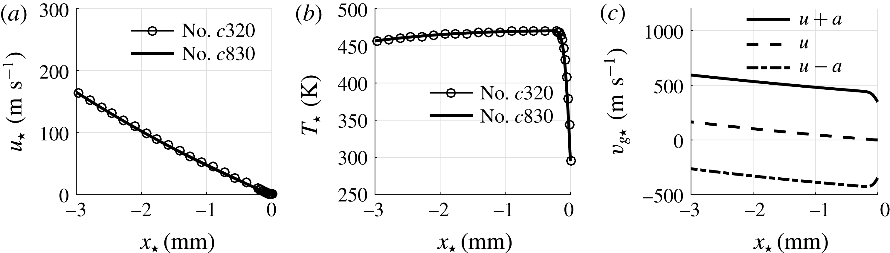
Furthermore, in figure 2(a,b) velocity and temperature comparison of two simulations of case up_h with different grids is shown. The case no.
 $c320$
indicates the solution using the grid utilized throughout this work for the lower Reynolds number flows, whereas for case no.
 $c830$
a much finer grid having 830 cells between shock wave and stagnation point along the axis of symmetry is used. Both simulations agree well.
Analysis of the flow field along the streamline between the shock wave and the stagnation point of case up_h: (a) axial velocity distribution for two different meshes, no.
 $c320$
and no.
 $c830$
indicate solutions using grids having 320 and 830 cells between shock wave and stagnation point along the axis of symmetry; (b) temperature distribution for two different meshes; (c) group velocities
 $v_{g\star }$
of the fast acoustic
 $u+a$
, a convective
 $u$
and the slow acoustic mode
 $u-a$
computed on grid no.
 $c320$
.

Properties of the unperturbed flow: Reynolds number
 $Re_{D}$
, stagnation point heat flux
 $\bar{q}$
, numerical (num) and experimental (exp) stagnation point heat flux from Ali et al. (Reference Ali, Zárate Cárdenas, Radespiel, Schilden and Schröder2018), period of a slow acoustic (
 $t_{sa}$
), entropy (
 $t_{en}$
) and fast acoustic (
 $t_{fa}$
) wave propagating between the shock wave and SPP at the axis of symmetry, frequency
 $f_{ac}=1/(t_{sa}+t_{fa})$
, Strouhal number
 $Sr_{ac}=Df_{ac}/u_{\infty }$
.

In figure 2(c) the group velocities
 $v_{g}$
of the slow acoustic (
 $u-a$
), entropy (
 $u$
) and fast acoustic wave (
 $u+a$
) of case up_h are plotted versus the axis of symmetry. From these distributions an a priori estimate of the acoustic standoff frequency can be calculated from the duration
 $t_{sa}+t_{fa}$
of an acoustic wave travelling upstream from the stagnation point to the shock wave as a slow acoustic wave and then back to the stagnation point as a fast acoustic wave. The values of
 $t_{sa}$
and
 $t_{fa}$
are calculated applying
 $$\begin{eqnarray}t_{i}=\int _{shock}^{sp}\frac{\text{d}x}{|v_{g,i}|}\end{eqnarray}$$
and the acoustic standoff frequency is
 $f_{ac}=1/(t_{sa}+t_{fa})$
. The values of
 $t_{sa}$
,
 $t_{fa}$
and
 $f_{ac}$
can be found in table 2 for both Reynolds numbers. The lower diameter probe from case up_l shows a higher standoff frequency
 $f_{ac}$
due to the smaller shock standoff distance. Non-dimensionalizing the standoff frequency to gain a standoff Strouhal number
 $Sr_{ac}$
leads to very similar values for both cases (table 2). The standoff frequency characterizes the superposition of waves downstream of the shock wave. Analogous to
 $t_{sa}$
and
 $t_{fa}$
, equation (4.1) can also be evaluated for a lower bound of
 $t_{en}$
, i.e. being an estimate for the duration of an entropy wave convecting at
 $v_{g}=u$
from the shock wave to the stagnation point, but the integration is truncated at the position of the maximum temperature. Close to the wall, the velocity tends to zero and diffusion, which is not accounted for in (4.1), is the mechanism of propagation. The values of
 $t_{en}$
are tabulated in table 2 and are one order of magnitude greater than the acoustic time scales owing to the low Mach number.
In the next step, to investigate the superposition of acoustic and entropy waves downstream of the shock wave, the impulse response of the SPP to acoustic and entropy disturbance modes is explored.
4.2 Impulse response
By inserting a single pulse of an incident slow acoustic, entropy and fast acoustic wave the modulation of the incident mode can be analysed without having to deal with the superposition of its reflections downstream of the shock wave. The incident single pulses are defined according to (3.1)–(3.6), where the argument
 $\unicode[STIX]{x1D719}=\boldsymbol{k}\boldsymbol{\cdot }\boldsymbol{x}-\unicode[STIX]{x1D714}t$
is processed by a filter
 $f(\unicode[STIX]{x1D719})$
 $$\begin{eqnarray}f(\unicode[STIX]{x1D719})=\left\{\begin{array}{@{}ll@{}}\unicode[STIX]{x1D719}-\unicode[STIX]{x1D719}_{0}+{\displaystyle \frac{\unicode[STIX]{x03C0}}{2}}, & \text{if }\unicode[STIX]{x1D719}_{0}-\unicode[STIX]{x03C0}<\unicode[STIX]{x1D719}<\unicode[STIX]{x1D719}_{0},\\ 0, & \text{else},\end{array}\right.\end{eqnarray}$$
with
 $\unicode[STIX]{x1D719}_{0}=\min (\boldsymbol{k}\boldsymbol{\cdot }\boldsymbol{x})-\unicode[STIX]{x1D714}t_{0}$
to yield a sinusoidally shaped pulse that enters the computational domain at the most upstream position with respect to the pulse propagation at the time
 $t_{0}$
. The single pulse can be traced and, provided the time scales
 $t_{sa}$
,
 $t_{fa}$
and
 $t_{en}$
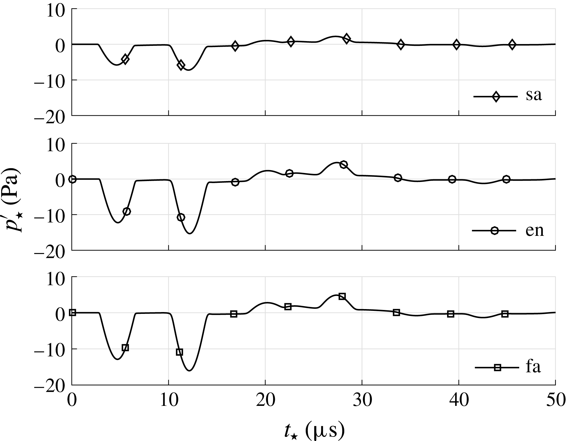
are known, the actual superposition can be elucidated. Time series of pressure and entropy fluctuations of cases sa_pulse_h (slow acoustic mode, incident pulse, high Reynolds number), en_pulse_h (entropy mode, incident pulse, high Reynolds number), and fa_pulse_h (fast acoustic mode, incident pulse, high Reynolds number) from table 1 at
 $x_{\star }=-1.5~\text{mm}$
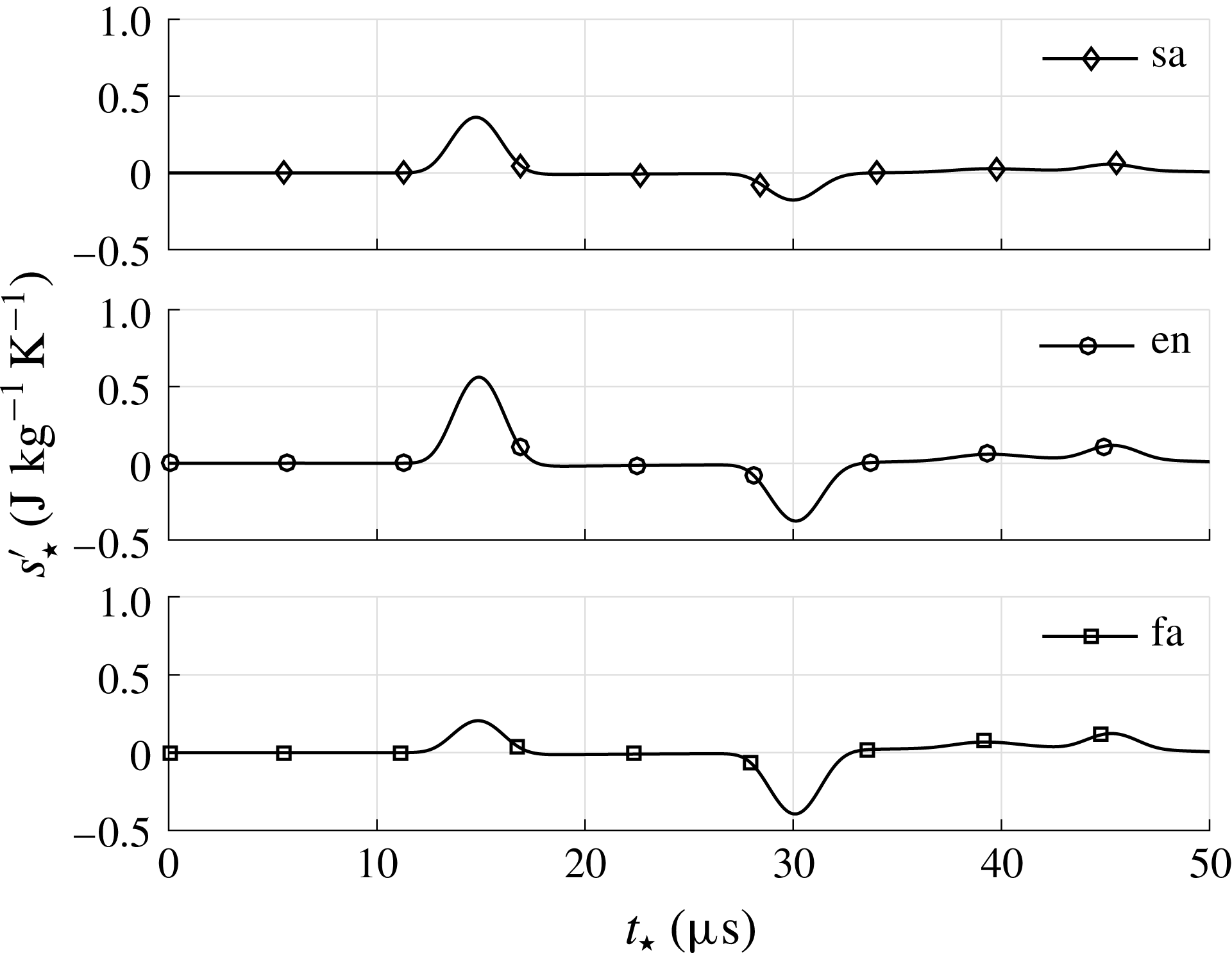
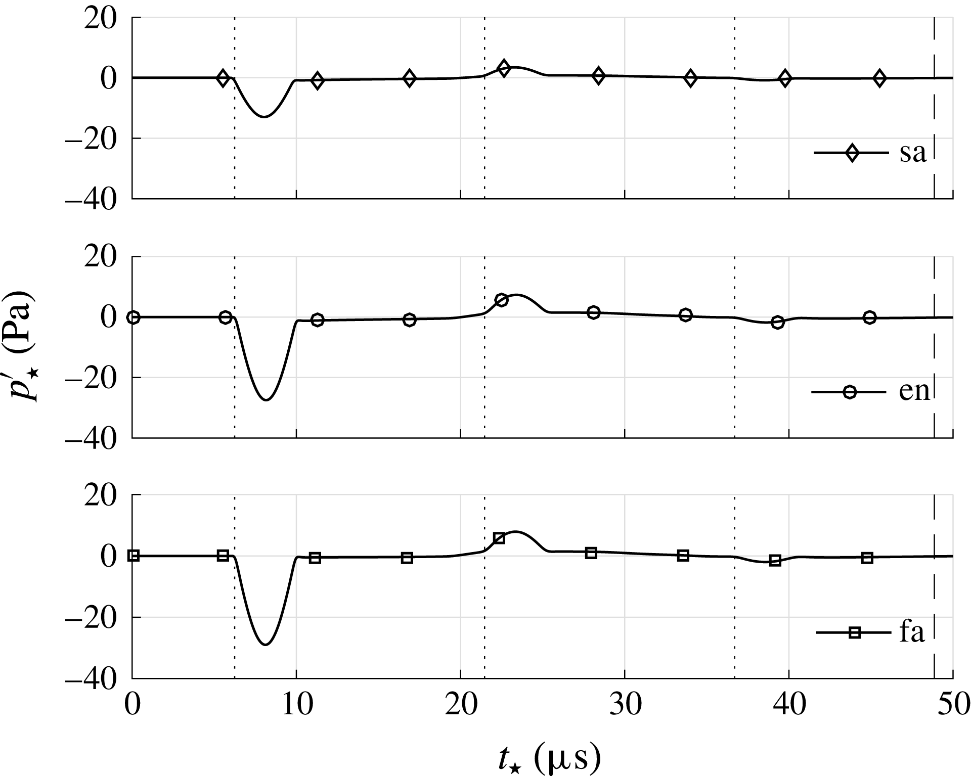
, i.e. approximately in the centre between shock wave and SPP are shown in figures 3 and 4 where each panel represents one of the three cases. It is obvious that all incident modes lead to acoustic and entropy waves downstream of the shock wave. The first pressure and entropy pulses at
 $t_{\star }=4.7~\unicode[STIX]{x03BC}\text{s}$
in figure 3 and
 $t_{\star }=14.7~\unicode[STIX]{x03BC}\text{s}$
in figure 4 represent the modulated incident wave. They are called the initial diverging acoustic and entropy wave and are generated simultaneously during the interaction of incident pulse and shock wave. Due to the different group velocities of acoustic and entropy waves they reach
 $x_{\star }=-1.5~\text{mm}$
at different times. For all incident modes, the initial diverging acoustic and entropy wave possess opposite signs. Their postshock modulation differs mainly by the absolute value of the ratio of the initial diverging acoustic and entropy wave. For the pressure fluctuations in figure 3, the second pulse at
 $t_{\star }=12~\unicode[STIX]{x03BC}\text{s}$
is caused by the reflection of the initial diverging acoustic wave at the SPP. It is called the first body reflected wave. Since
 $x_{\star }=-1.5~\text{mm}$
is approximately in the centre between the shock wave and the SPP, the time between the first and second pulse is close to
 $(t_{sa}+t_{fa})/2$
. The third pulse at
 ${\approx}20~\unicode[STIX]{x03BC}\text{s}$
follows from the reflection of the body reflected wave at the shock wave. It is denoted the first shock reflected wave. Again, the time between the second and third pulse is
 $(t_{sa}+t_{fa})/2$
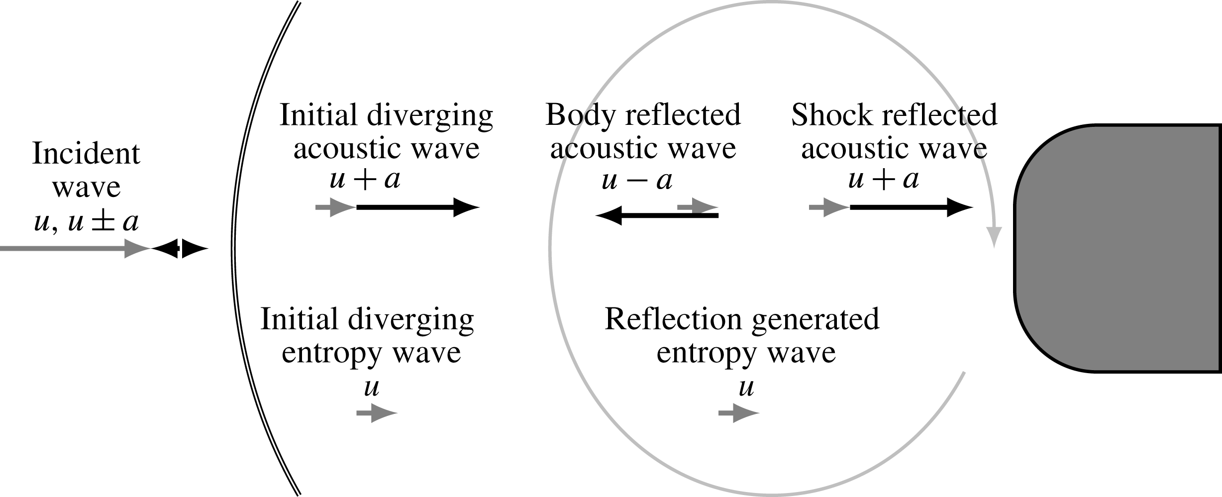
. This kind of propagation of the postshock acoustic wave continues, i.e. it is damped during its reflection at the shock wave and slightly amplified during the reflection at the SPP. The reflection at the shock wave leads to a change of sign of the pressure disturbance. A schematic diagram of the acoustic wave pattern is illustrated in the upper half of figure 5.
Time traces of pressure fluctuations at
 $x_{\star }=-1.5~\text{mm}$
between the shock wave and the stagnation point for an incident pulse of the slow acoustic (sa_pulse_h), entropy (en_pulse_h) and fast acoustic (fa_pulse_h) mode.

Time traces of entropy fluctuations at
 $x_{\star }=-1.5~\text{mm}$
between the shock wave and the stagnation point for an incident pulse of the slow acoustic (sa_pulse_h), entropy (en_pulse_h) and fast acoustic mode (fa_pulse_h).

Acoustic and entropy mode wave pattern for any incident mode. All incident modes directly lead to initial diverging fast acoustic and entropy waves. The acoustic wave travels between the shock wave and the SPP alternating as fast and slow acoustic mode. The reflection of the acoustic wave at the shock wave generates a further entropy wave.

Postshock waves for all incident mode types at
 $x_{\star }=-1.5~\text{mm}$
; pressure amplitude
 $\hat{p}_{i,\star }$
of the initial diverging acoustic wave at
 $t_{\star }=4.7~\unicode[STIX]{x03BC}\text{s}$
; entropy amplitude
 ${\hat{s}}_{i,\star }$
of the initial diverging entropy wave at
 $t_{\star }=14.7~\unicode[STIX]{x03BC}\text{s}$
; non-dimensional ratio of the initial diverging acoustic and entropy wave
 ${\hat{s}}_{i}/\hat{p}_{i}$
; entropy amplitude of the first reflection generated entropy wave
 ${\hat{s}}_{g,\star }$
at
 $t_{\star }=30~\unicode[STIX]{x03BC}\text{s}$
.

The entropy disturbances in figure 4 show a different pattern. The second pulse at
 $t_{\star }=30~\unicode[STIX]{x03BC}\text{s}$
follows the initial diverging entropy wave with a lag of
 $t_{sa}+t_{fa}$
. It is generated during the reflection of the body reflected acoustic wave at the shock wave. It is called the first reflection generated entropy wave and the disturbance has the same sign as the body reflected acoustic wave. The schematic diagram of the entropy wave pattern is included in the lower half of figure 5.
The magnitudes of the initial diverging acoustic
 $\hat{p}_{i}$
and entropy
 ${\hat{s}}_{i}$
waves and their non-dimensional ratio are summarized in table 3. All incident modes lead to different ratios of the initial diverging acoustic and entropy waves
 $({\hat{s}}_{i}/\hat{p}_{i})(a_{0}^{2}\unicode[STIX]{x1D70C}_{0}/c_{p})$
and deviate by at least 36 %. This is a necessary condition for any modal decomposition that relies on the measurement of quantities caused by postshock acoustic and entropy waves such as pressure and heat flux fluctuations.
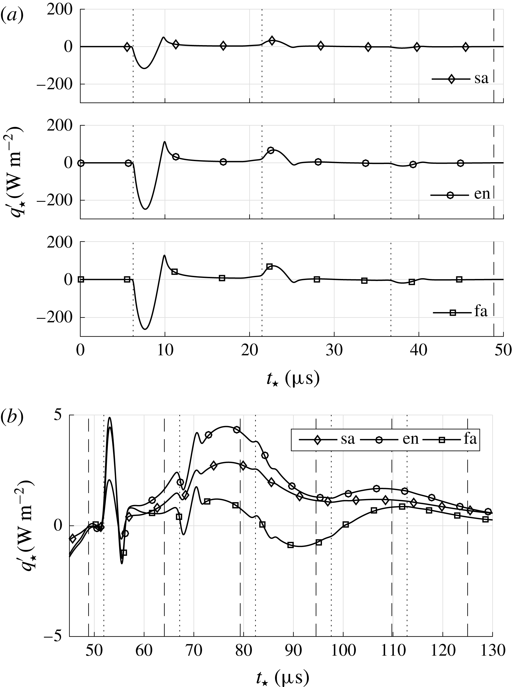
Time series of the stagnation point pressure and heat flux disturbances of cases sa_pulse_h, en_pulse_h and fa_pulse_h are shown in figures 6 and 7. In all panels, the vertical thin dotted lines represent multiples of
 $t_{sa}+t_{fa}$
, where the initial line is defined by the first detection of the initial diverging acoustic wave at
 $t_{\star }=6.1~\unicode[STIX]{x03BC}\text{s}$
. The vertical thin dashed lines in figures 6 and 7(a), and its first occurrence in figure 7(b) represent the lower bound
 $t_{en}$
. The following dashed lines in figure 7(b) represent further multiples of
 $t_{sa}+t_{fa}$
. The time between the first dashed line at
 $t_{\star }=48.3~\unicode[STIX]{x03BC}\text{s}$
and the first dotted line is
 $t_{en}-t_{fa}$
, thus giving a lower bound for the first appearance of the initial diverging entropy wave in any signal. As discussed before, the stagnation point pressure in figure 6 shows for all incident modes postshock acoustic mode related pulses with alternating sign. The acoustic wave diminishes to a very low level before the entropy wave can reach the SPP. The postshock entropy waves related pressure disturbance is negligible. The stagnation point heat flux in figure 7(a) also shows pulses caused by the postshock acoustic wave after the thin dotted lines. Since pressure and heat flux signals are not proportional, i.e. the heat flux pulses exhibit a visible undershoot after the main pulse, an additional mechanism leads to a more complex transfer function between postshock acoustic wave and heat flux fluctuation. This issue will be addressed later.
Time traces of pressure fluctuations caused by postshock acoustic waves at the stagnation point for an incident pulse of the slow acoustic (sa_pulse_h), entropy (en_pulse_h) and fast acoustic (fa_pulse_h) mode.

Time traces at the stagnation point heat flux fluctuations caused by postshock acoustic and entropy waves for an incident pulse of the slow acoustic (sa_pulse_h), entropy (en_pulse_h) and fast acoustic (fa_pulse_h) mode: (a) time trace beginning at
 $t_{\star }=0$
showing mainly the contribution of the postshock acoustic wave to the heat flux fluctuation; (b) detailed view of the entropy mode contribution to the heat flux fluctuation.

Increasing the scale of the heat flux for a subsequent time span in figure 7(b) emphasises the contribution of the initial diverging entropy wave. As in figure 7(a), the postshock acoustic wave related heat flux fluctuations appear as local extrema immediately after the thin dotted lines. For
 $t_{\star }>80~\unicode[STIX]{x03BC}\text{s}$
, they are hardly noticeable. The remaining heat flux deviations for
 $t>t_{en}$
are caused by the postshock entropy waves, i.e. the initial diverging entropy wave and the reflection generated entropy waves that follow in intervals of
 $t_{sa}+t_{fa}$
. Unlike the postshock acoustic wave related heat flux, distinct responses to singular postshock entropy waves appearing in intervals of
 $t_{sa}+t_{fa}$
cannot be observed. The transfer function between postshock entropy waves and heat flux fluctuations causes heat flux responses to the individual postshock entropy waves that sustain longer than the period of the inserted pulse and
 $t_{sa}+t_{fa}$
. Therefore, the responses to the individual postshock entropy waves merge and form the trend that is characterized by a local maximum around
 $73~\unicode[STIX]{x03BC}\text{s}$
. The peak heat flux fluctuation can be linked to the amplitude of the initial diverging entropy wave
 ${\hat{s}}_{i,\star }$
in table 3. At growing initial diverging entropy wave, the peak heat flux fluctuation increases. The following decay of the heat flux deviation is related to the first reflection generated entropy wave
 ${\hat{s}}_{g,\star }$
from table 3. In addition to the different behaviour of the transfer functions between postshock acoustic and entropy waves and heat flux fluctuations, the magnitude differs tremendously. The contribution of the postshock entropy waves to the heat flux fluctuations is lower than the contribution of the postshock acoustic wave.
As aforementioned, an additional mechanism causes the transfer function of acoustic waves to heat flux fluctuations to be not directly proportional. The necessity of this further mechanism can also be deduced from the isothermal boundary conditions enforcing
 $T^{\prime }=0$
and the isentropic relations demanding
 $T^{\prime }\propto p^{\prime }$
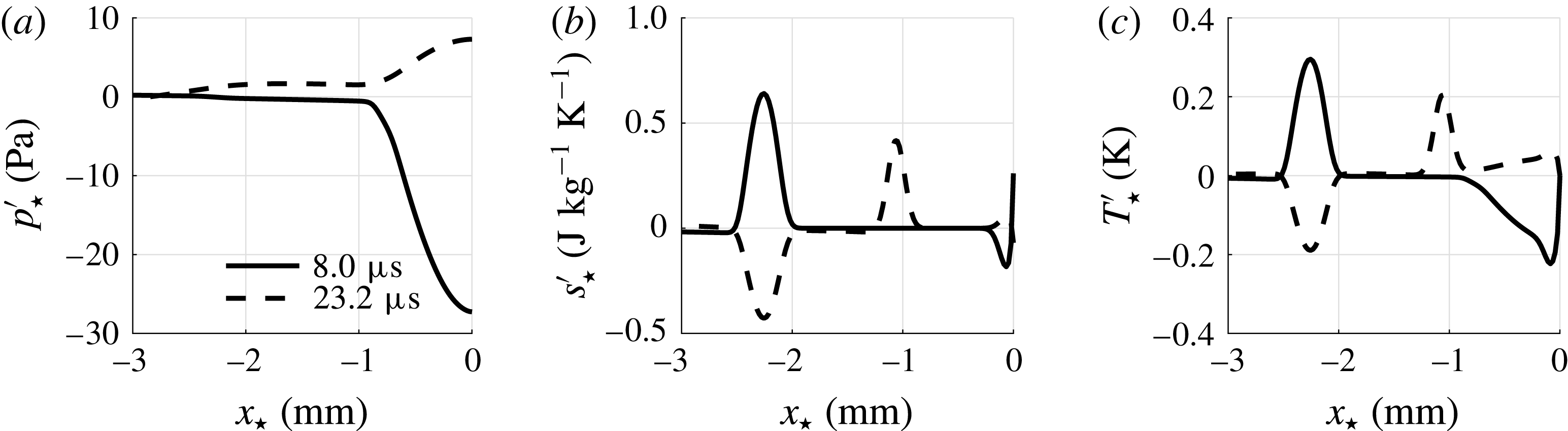
for acoustic waves. To determine the intermediate step between an acoustic wave and the heat flux, instantaneous pressure, entropy and temperature distributions on the axis of symmetry of case en_pulse_h are shown in figure 8 at two time instances
 $7.8~\unicode[STIX]{x03BC}\text{s}$
and
 $23~\unicode[STIX]{x03BC}\text{s}$
. The pressure disturbance in figure 8(a) exhibits its first and second temporal extremum, while the entropy wave in figure 8(b) did not reach the SPP, yet. Nonetheless, entropy fluctuations are evident close to the surface of the SPP. To fulfil the isothermal boundary condition in the presence of an acoustic wave reflecting at the wall as shown in figure 8(c), an entropy spot is generated close to the wall. When the acoustic wave travels upstream again, the entropy spot related temperature disturbance remains close to the wall and is balanced by diffusion, i.e. additional heat flux on the surface, causing the heat flux signal of figure 7(a) to show the aforementioned undershoot.
Instantaneous flow field between the shock wave and the stagnation point for an incident pulse of the entropy mode (en_pulse_h); (a) pressure fluctuations caused by the postshock acoustic wave; (b) entropy fluctuations caused by the postshock entropy waves; (c) temperature fluctuations caused by the postshock acoustic wave and the postshock entropy waves.

It can be concluded that all types of incident disturbance modes lead to an initial diverging acoustic and entropy wave, whose ratio differs. However, for all incident modes the ratio has a negative sign, i.e. the waves possess a phase shift of
 $\unicode[STIX]{x03C0}$
. Moreover, the heat flux fluctuations show contributions of the postshock acoustic wave and the postshock entropy waves. However, the initial diverging entropy wave of all incident modes led to lower heat flux amplitudes than the initial diverging acoustic wave. Using the findings of §§ 4.1 and 4.2 a model equation is derived to investigate the superposition of single disturbance pulses onto continuous incident disturbance modes.
4.3 Model equation
Assuming weak continuous sinusoidal incident modes, the stagnation point pressure and heat flux fluctuations can be modelled as a linear superposition of the contributions of the postshock acoustic and entropy waves to each fluctuating quantity, e.g. see Morkovin (Reference Morkovin1960) for a similar model for pressure fluctuations. The model equations for pressure and heat flux fluctuations are formulated based on the time scales
 $t_{fa}+t_{sa}$
and
 $t_{en}$
deduced from the mean flow listed in table 2 and the postshock wave pattern extracted from the impulse response shown in figure 5. The amplitudes of the initial diverging acoustic wave
 $\hat{p}_{i}$
and the initial diverging entropy wave
 ${\hat{s}}_{i}$
also appear in the model equation and represent the input of the different incident waves, thus causing different pressure and heat flux fluctuations for various incident waves.
First, the model equation for pressure fluctuations is formulated. It reads
 $$\begin{eqnarray}p^{\prime }=2\hat{p}_{i}\text{e}^{\text{i}\unicode[STIX]{x1D714}t}\mathop{\sum }_{j=0}^{\infty }c_{I}^{j}\text{e}^{-\text{i}\unicode[STIX]{x1D714}j(t_{sa}+t_{fa})}.\end{eqnarray}$$
The first term for
 $j=0$
denotes the pressure fluctuation induced by the initial diverging acoustic wave. The terms for
 $j>0$
represent the shock reflected acoustic waves where the factor
 $c_{I}$
is the transfer function of an acoustic wave being reflected at the shock wave.
According to Chaudhry & Candler (Reference Chaudhry and Candler2016)
 $c_{I}$
depends on the Mach number and for
 $\unicode[STIX]{x1D6FE}=1.4$
, it is
 $-0.139<c_{I}<0$
. The argument
 $-\unicode[STIX]{x1D714}j(t_{sa}+t_{fa})$
of (4.3) introduces the phase shift of the impinging postshock acoustic waves at the stagnation point. It depends on the angular frequency of the incident disturbance and gives rise to interference. Furthermore, the factor 2 accounts for the contribution of the body reflected acoustic waves to the pressure fluctuations. At the wall, the velocity fluctuation is zero
 $u^{\prime }=0$
. Therefore, velocity fluctuations due to fast acoustic waves approaching the wall
 $u_{fa}^{\prime }$
and their reflections
 $u_{sa}^{\prime }$
, i.e. slow acoustic waves moving upstream away from the wall, need to cancel out
 $u_{fa}^{\prime }+u_{sa}^{\prime }=0$
. Using (3.2) to relate velocity and pressure fluctuations, we obtain identical pressure fluctuations of approaching and reflected wave, thus we account for all body reflected waves by introducing a factor of 2. Note that (4.3) assumes the amplitude of the postshock acoustic waves to be altered only by the interaction with the shock wave. Changes of the amplitude due to the non-uniform flow or the isothermal wall boundary condition are neglected. The postshock entropy waves do not contribute to pressure fluctuations.
The resonant behaviour of the pressure frequency response can be deduced from (4.3). The phase of the individual summands
 $\unicode[STIX]{x1D719}_{j}$
is
 $$\begin{eqnarray}\unicode[STIX]{x1D719}_{j}=j(\unicode[STIX]{x03C0}-\unicode[STIX]{x1D714}(t_{sa}+t_{fa})).\end{eqnarray}$$
At multiples of the acoustic standoff frequency
 $f_{ac}$
the postshock acoustic waves interfere destructively since
 $\arg (c_{I})=\unicode[STIX]{x03C0}$
. Constructive interference occurs at frequencies
 $f=f_{ac}/2+nf_{ac}$
with
 $n\in \mathbb{N}$
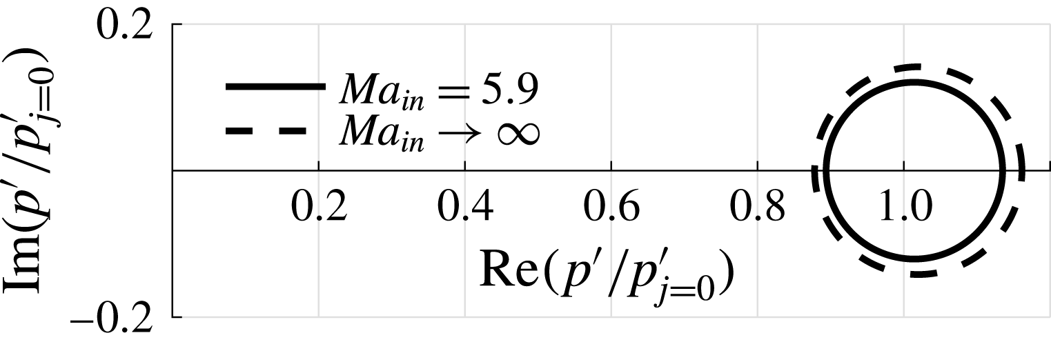
. The Nyquist plot of (4.3) for
 $Ma=5.9$
is shown in figure 9. The outer locus denotes the hypersonic limit
 $Ma_{in}\rightarrow \infty$
of
 $c_{I}=-0.139$
. The rightmost intersections of the frequency response loci with the real axis resemble constructive interference, whereas the intersections on the left denote destructive superposition. Due to the intense damping of the body reflected acoustic wave, the phase difference of the final pressure signal compared to the initial diverging wave at
 $\arg (p^{\prime }/p_{j=0}^{\prime })$
is limited to small values. Furthermore, since in the case of constructive interference all summands have the same sign and for destructive interference the signs change alternately, the constructive interference can be expected to be more intense. This result is indicated in figure 9. The initial diverging acoustic wave
 $p_{j=0}^{\prime }$
at
 $1+0\text{i}$
does not coincide with the centre of the intersections of the frequency response locus on the real axis.
Nyquist plot of the net pressure signal of (4.3); the inner locus shows the
 $\unicode[STIX]{x1D714}$
dependency at
 $Ma_{in}=5.9$
, the outer locus denotes the hypersonic limit
 $Ma_{in}\rightarrow \infty$
of
 $c_{I}=-0.139$
for
 $\unicode[STIX]{x1D6FE}=1.4$
.

To model the heat flux signal, the contribution of the combined pressure signal to the heat flux fluctuations can be written
 $$\begin{eqnarray}q_{ac}^{\prime }=c_{\mathit{II}}p^{\prime },\end{eqnarray}$$
where the factor
 $c_{\mathit{II}}$
is the transfer function between the pressure and pressure related heat flux fluctuations shown in figure 7(a). It contains the phase shift caused by the intermediate step of entropy generation and a potential decay with increasing frequency. The contribution of the postshock entropy waves, i.e. the initial diverging entropy wave and the reflection generated entropy waves, to the heat flux fluctuations is expressed as
 $$\begin{eqnarray}q_{en}^{\prime }=c_{\mathit{III}}({\hat{s}}_{i}\text{e}^{\text{i}\unicode[STIX]{x1D714}(t-(t_{en}-t_{fa}))}+c_{\mathit{IV}}p^{\prime }\text{e}^{-\text{i}\unicode[STIX]{x1D714}(t_{en}+t_{sa})}).\end{eqnarray}$$
In (4.6),
 $c_{\mathit{III}}$
is the transfer function linking entropy waves and their heat flux fluctuation contribution. The transfer function
 $c_{\mathit{IV}}$
relates body reflected acoustic waves and reflection generated entropy waves. According to McKenzie & Westphal (Reference McKenzie and Westphal1968) and figures 3 and 4
 $c_{\mathit{IV}}$
is a positive real number. The arguments of both terms in (4.6) depend on the entropy wave time scale to consider the phase shift that results from the different group velocities of the postshock acoustic and entropy waves. Note that the reflection generated entropy waves follow from reflections of body reflected acoustic waves and are unlike the shock reflected acoustic waves not necessarily weaker than the initial diverging wave which is evident by the values of
 ${\hat{s}}_{i}$
and
 ${\hat{s}}_{g}$
in table 3. For the incident fast acoustic wave case fa_pulse_h, the absolute value of the reflection generated entropy wave
 ${\hat{s}}_{g}$
is higher than that of the initial diverging entropy wave
 ${\hat{s}}_{i}$
. Even though the amplitude ratio of the initial diverging entropy wave and the subsequent reflection generated entropy waves is not universal for all incident modes, their phase difference
 $\unicode[STIX]{x0394}\unicode[STIX]{x1D719}_{en}$
is. Using
 $\arg ({\hat{s}}_{i})=\unicode[STIX]{x03C0}$
it can be written
 $$\begin{eqnarray}\unicode[STIX]{x0394}\unicode[STIX]{x1D719}_{en}=\unicode[STIX]{x03C0}+\unicode[STIX]{x1D714}(t_{fa}+t_{sa})-\arg (p^{\prime }).\end{eqnarray}$$
In the case of destructive pressure interference
 $\unicode[STIX]{x0394}\unicode[STIX]{x1D719}_{en}=\unicode[STIX]{x03C0}$
holds and thus also destructive entropy wave interference occurs for the postshock entropy wave related heat flux. For constructive pressure interference follows
 $\unicode[STIX]{x0394}\unicode[STIX]{x1D719}_{en}=0$
resulting in constructive postshock entropy wave interference, too. Besides sheer destructive and constructive interference, the net phase of the postshock acoustic waves
 $\arg (p^{\prime })$
leads to a nonlinearity in
 $\unicode[STIX]{x0394}\unicode[STIX]{x1D719}_{en}(\unicode[STIX]{x1D714})$
which increases at decreasing damping due to
 $c_{I}$
as can be seen in figure 9. Rearranging the terms of (4.5) and (4.6), the full heat flux signal
 $q^{\prime }=q_{ac}^{\prime }+q_{en}^{\prime }$
can be written
 $$\begin{eqnarray}q^{\prime }=c_{\mathit{III}}{\hat{s}}_{i}\text{e}^{\text{i}\unicode[STIX]{x1D714}t}\text{e}^{-\text{i}\unicode[STIX]{x1D714}(t_{en}-t_{fa})}+p^{\prime }(c_{\mathit{II}}+c_{\mathit{III}}c_{\mathit{IV}}\text{e}^{-\text{i}\unicode[STIX]{x1D714}(t_{en}+t_{sa})}).\end{eqnarray}$$
It is evident from (4.8) that besides the direct contribution of the postshock acoustic waves to the heat flux via
 $c_{\mathit{II}}$
also a certain part of the postshock entropy wave related heat flux, i.e. the third term due to reflection generated entropy waves, must be attributed to the postshock acoustic waves. Since in the postshock region various types of incident modes differ mainly by their amplitude ratio of the initial diverging pressure and entropy wave
 $\hat{p}_{i}/{\hat{s}}_{i}$
, the initial diverging entropy wave, i.e. the first term on the right-hand side of (4.8), needs to be measured by the heat flux transducer to differentiate between varying incident modes from their SPP pressure and heat flux signal. This makes the properties of the transfer function
 $c_{\mathit{III}}$
a crucial factor whenever a differentiation between various incident modes is required, i.e. for
 $c_{\mathit{III}}=0$
, a modal decomposition based on the differing ratios of the initial diverging acoustic and entropy waves cannot be posed since the initial diverging entropy wave is not captured in any signal.
In the following section, a further investigation of
 $c_{\mathit{III}}$
is pursued based on control theory. The step response is analysed to make a statement concerning the heat flux frequency response of an SPP to postshock entropy waves.
4.4 Step response
The step response of the heat flux sensor to postshock entropy waves is analysed to better understand the properties of the transfer function
 $c_{\mathit{III}}$
. Such a step response can be initiated by a sudden change of entropy, i.e. density at constant pressure, of the fluid surrounding the probe at the steady state. Considering the stagnation point heat flux, this change of state leads to a change of the local Reynolds number. An expansion of the Reynolds number, i.e. the total derivative, for small changes of entropy reads
 $$\begin{eqnarray}\text{d}Re=-Re\left(\left.1+\frac{T}{\unicode[STIX]{x1D702}}\frac{\text{d}\unicode[STIX]{x1D702}}{\text{d}T}\right|_{T}\right)\frac{\text{d}s}{c_{p}}.\end{eqnarray}$$
The sudden change of the Reynolds number causes an imbalance of viscous and inviscid terms of the governing equations in the thermal boundary layer, i.e. the heat flux response shows the reestablishment to a new equilibrium. Besides the desired response of the thermal boundary layer, the sudden change of entropy at the inflow causes a Mach number deviation
 $$\begin{eqnarray}\text{d}Ma=-\frac{Ma}{2}\frac{\text{d}s}{c_{p}},\end{eqnarray}$$
which in turn results in a new steady state pressure field downstream of the shock wave. The acoustic wave that propagates downstream of the shock wave during the convergence of the pressure field leads to heat flux disturbances via
 $c_{\mathit{II}}$
and conceals the heat flux step response to the change of entropy. To avoid this, two different approaches are proposed.
First, for cases en_flood_l and en_flood_h the entropy wave inflow boundary condition from (3.5) is modified as
 $$\begin{eqnarray}\unicode[STIX]{x1D70C}^{\prime }=\unicode[STIX]{x1D700}\unicode[STIX]{x1D70C}_{\infty }\tanh (\boldsymbol{k}\boldsymbol{\cdot }\boldsymbol{x}-\unicode[STIX]{x1D714}t).\end{eqnarray}$$
This approach is referred to as ‘flood’ since the computational domain is flooded with an entropy wave. Applying the entropy flooding, the Mach number deviation at the inflow still causes postshock acoustic wave related heat flux fluctuations during the pressure field convergence, but the entropy flood heat flux response is temporally shifted to times
 $t>t_{en}$
and the overlap of both heat flux contributions can be reduced. On the other hand, equation (4.11) does not resemble a discontinuous step function for the entropy and even if it were, the discontinuity would be smeared by diffusion during the convection from the inflow to the SPP.
Therefore, in the second approach, a rather non-physical numerical experiment is performed in cases step_l and step_h by restarting a converged simulation with a slightly altered Reynolds number. Similar to a sudden change of entropy, the equilibrium between viscous and inviscid terms of the governing equations is disturbed and the immediate heat flux response shows the desired reestablishment of a new equilibrium in the thermal boundary layer. Due to the temporal discontinuity introduced into the governing equations by the slight change of Reynolds number, this approach is referred to as ‘step’.
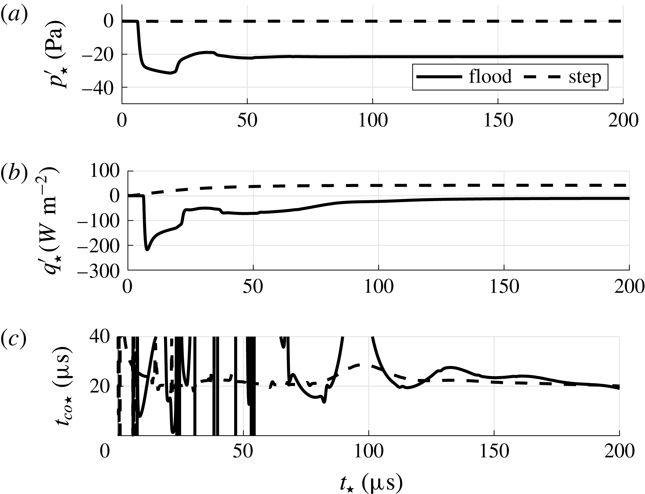
In figure 10(a,b), the response of the stagnation point pressure and heat flux signals to the aforementioned approaches of cases en_flood_h and step_h are shown. For the case en_flood_h the stagnation point pressure and heat flux converge to a new steady state. As soon as the incident entropy wave interacts with the shock, it generates the aforementioned acoustic wave and the pressure in figure 10(a) drops within the time scale of the fast acoustic wave
 $t_{fa}$
. Then, only the postshock acoustic waves can be seen as they diminish during the convergence. The heat flux step response in figure 10(b) shows for the en_flood_h case two time scales during its convergence. First, it rapidly changes due to the altered Mach number and postshock pressure. Then, starting at
 $t_{\star }\approx 60~\unicode[STIX]{x03BC}\text{s}$
the entropy flood leads to a slow increase of the heat flux. This second part of the convergence is related to the slight change of the local Reynolds number in the thermal boundary layer. For the case step_h, the pressure response is zero since the pressure at rest does not depend on the Reynolds number. The development of a new heat flux equilibrium shows the same behaviour as the entropy flood related part of the step response of the case en_flood_h. The asymptotic trend of the heat flux step response resembles the behaviour of a low pass filter. The transfer function of a low pass filter is
 $$\begin{eqnarray}G(\text{i}\unicode[STIX]{x1D714})=\frac{K}{1+\text{i}\unicode[STIX]{x1D714}t_{co}},\end{eqnarray}$$
thus leading to a strong decrease of
 $|G|$
beyond
 $\unicode[STIX]{x1D714}>2\unicode[STIX]{x03C0}/t_{co}$
. The cutoff frequency
 $f_{co}=1/t_{co}$
can be determined from the step response via
 $$\begin{eqnarray}t_{co}=\frac{\unicode[STIX]{x2202}t}{\unicode[STIX]{x2202}q^{\prime }}(q_{\infty }^{\prime }-q^{\prime }).\end{eqnarray}$$
The distribution of
 $t_{co}$
based on (4.13) from the data of figure 10(b) is shown in figure 10(c). For the case en_flood_h, the diminishing postshock acoustic wave related heat flux fluctuations render the application of (4.13) impossible. However, for times
 $t_{\star }>100~\unicode[STIX]{x03BC}\text{s}$
and the data of case step_h a value of approximately
 $20~\unicode[STIX]{x03BC}\text{s}$
can be obtained.
Step response at the stagnation point for the cases of entropy mode flooding (en_flood_h) and a slight change of Reynolds number (step_h) at
 $Re=109\,375$
; (a) pressure response; (b) heat flux response; (c) cutoff frequency evaluation by (4.13).

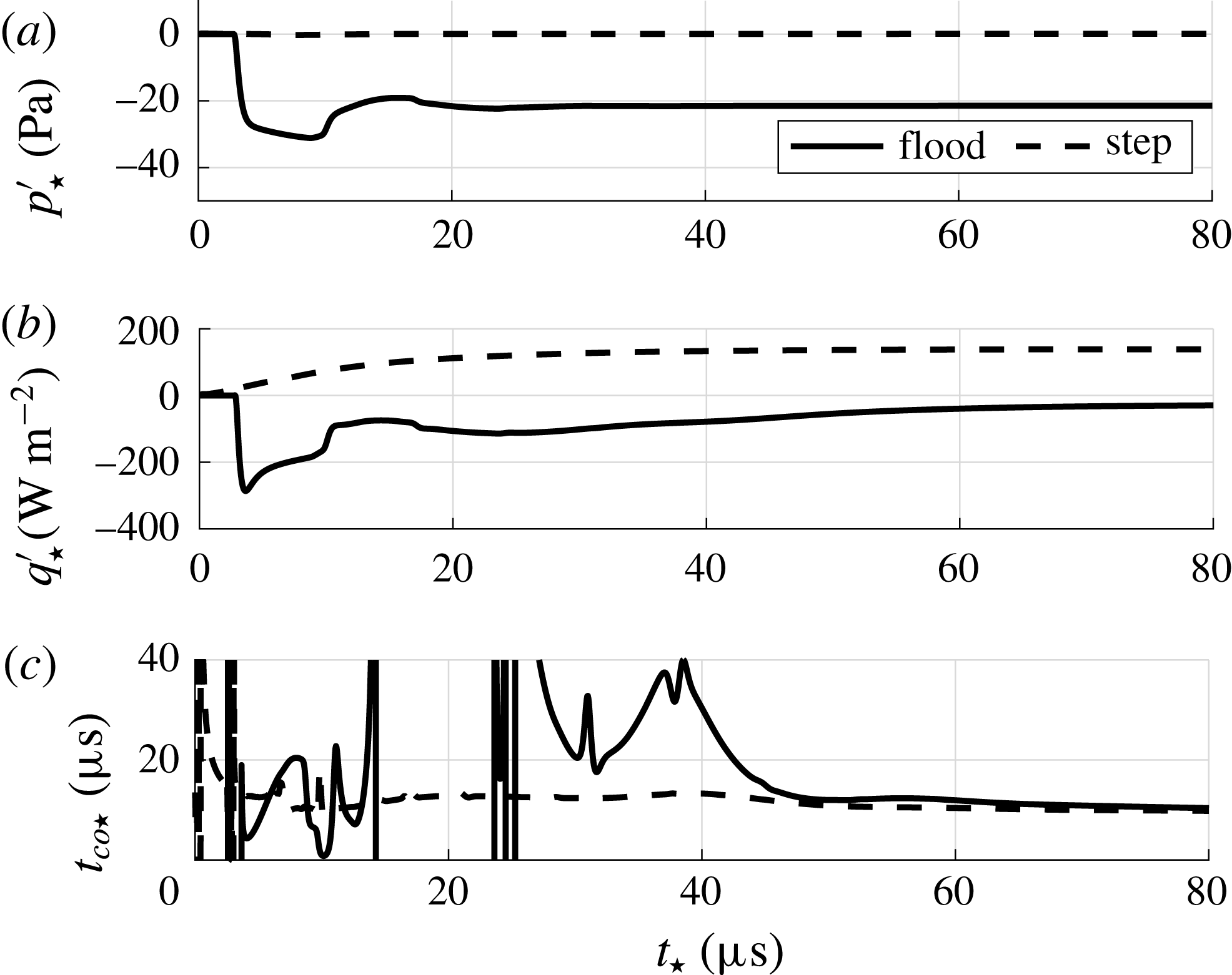
The analogous analysis for the lower Reynolds number cases en_flood_l and step_l is depicted in figure 11. For the smaller SPP, a value of approximately
 $12~\unicode[STIX]{x03BC}\text{s}$
can be extracted. All values for the cutoff time scale
 $t_{co}$
, cutoff frequency
 $f_{co}$
and cutoff Strouhal number
 $Sr_{D,co}$
are listed in table 4. The non-dimensional analysis shows a decreasing cutoff Strouhal number at decreasing Reynolds number. On the other hand, from the Strouhal number itself we can directly deduce that smaller SPPs lead to higher cutoff frequencies. The final cutoff frequency in table 4 shows the latter trend determined by the Strouhal number definition. The Reynolds number effect is benevolent but too weak to yield higher cutoff frequencies using larger SPP.
Step response at the stagnation point for the cases of entropy mode flooding (en_flood_l) and a slight change of Reynolds number (step_l) at
 $Re=50\,000$
; (a) pressure response; (b) heat flux response; (c) cutoff frequency evaluation by (4.13).

Properties of the heat flux response to entropy waves, i.e. the transfer function
 $c_{\mathit{III}}$
modelled as a low pass filter; Reynolds number
 $Re_{D}=\unicode[STIX]{x1D70C}_{\infty }u_{\infty }D/\unicode[STIX]{x1D702}_{\infty }$
, cutoff time scale
 $t_{co}$
, cutoff frequency
 $f_{co}$
and cutoff Strouhal number
 $Sr_{D,co}=f_{co}D/u_{\infty }$
.

Regarding the transient behaviour of the heat flux sensor, it can be concluded that the transfer function
 $c_{\mathit{III}}$
connecting postshock entropy waves and heat flux fluctuations can be expected to behave like a low pass filter. From the findings in § 4.3, i.e. the initial diverging entropy wave has to be measured by the heat flux sensor to differentiate between the incident mode types based on heat flux and pressure signal, we can expect the SPP frequency response to different incident mode types to be identical above the determined cutoff frequency. The analysis of the frequency response is given in the next section.
4.5 Frequency response
To determine the frequency response, continuous waves of the fast acoustic, slow acoustic and entropy mode at different frequencies are superimposed to the flow. The cases of this investigation are denoted continuous in table 1. The frequencies of the investigation are based on the expected resonant behaviour of the larger heat flux SPP from the case up_h. Five Strouhal numbers are chosen to cover the frequency range up to the second destructive interference of postshock acoustic waves. Since the response coefficients of the pressure and heat flux fluctuations are required at a certain unit Reynolds number and frequency, lower Strouhal numbers result for the smaller pressure SPP from the case up_l. The non-dimensional analysis of the unperturbed flow in § 4.1 showed very similar Strouhal numbers dictating the resonant behaviour. Therefore, the Strouhal numbers for the smaller pressure SPP cover a smaller non-dimensional range.
In the subsequent analysis of the frequency response, the response coefficients
 $r_{j,i}$
of the transfer matrix
 $\unicode[STIX]{x1D64E}$
 $$\begin{eqnarray}\unicode[STIX]{x1D64E}=\left(\begin{array}{@{}cc@{}}r_{p,ac} & r_{p,en}\\ r_{q,ac} & r_{q,en}\end{array}\right)\end{eqnarray}$$
in the ansatz
 $\boldsymbol{F}_{w}=\unicode[STIX]{x1D64E}\boldsymbol{F}_{\infty }$
for the modal decomposition are utilized. The complete non-dimensional definition of the modal decomposition using fluctuations reads
 $$\begin{eqnarray}\left(\begin{array}{@{}c@{}}{\displaystyle \frac{p_{w}^{\prime }}{\bar{p}_{w}}}\\ {\displaystyle \frac{q_{w}^{\prime }}{\bar{q}_{w}}}\end{array}\right)=\left(\begin{array}{@{}cc@{}}{\displaystyle \frac{p_{w}^{\prime }\bar{\unicode[STIX]{x1D70C}}_{\infty }}{\bar{p}_{w}\unicode[STIX]{x1D70C}_{\infty ,ac}^{\prime }}} & {\displaystyle \frac{p_{w}^{\prime }\bar{\unicode[STIX]{x1D70C}}_{\infty }}{\bar{p}_{w}\unicode[STIX]{x1D70C}_{\infty ,en}^{\prime }}}\\ {\displaystyle \frac{q_{w}^{\prime }\bar{\unicode[STIX]{x1D70C}}_{\infty }}{\bar{q}_{w}\unicode[STIX]{x1D70C}_{\infty ,ac}^{\prime }}} & {\displaystyle \frac{q_{w}^{\prime }\bar{\unicode[STIX]{x1D70C}}_{\infty }}{\bar{q}_{w}\unicode[STIX]{x1D70C}_{\infty ,en}^{\prime }}}\end{array}\right)\left(\begin{array}{@{}c@{}}{\displaystyle \frac{\unicode[STIX]{x1D70C}_{ac}^{\prime }}{\bar{\unicode[STIX]{x1D70C}}_{\infty }}}\\ {\displaystyle \frac{\unicode[STIX]{x1D70C}_{en}^{\prime }}{\bar{\unicode[STIX]{x1D70C}}_{\infty }}}\end{array}\right).\end{eqnarray}$$
In this formulation, both incident disturbances in
 $\boldsymbol{F}_{\infty }$
are quantified by their density fluctuation to yield a common frame of reference for the response coefficients. The response coefficients
 $r_{j,i}$
depend on the Strouhal number and are complex numbers to account for phase differences between incident waves and stagnation point fluctuations, i.e. for a single Strouhal number (4.15) is correct in time. To apply the decomposition to experimental power spectral density (PSD) distributions or bandwidth filtered nRMS values, equation (4.15) is converted into an nRMS formulation assuming uncorrelated acoustic and entropy waves in the free stream
 $$\begin{eqnarray}\left(\begin{array}{@{}c@{}}\langle p_{w}\rangle ^{2}\\ \langle q_{w}\rangle ^{2}\end{array}\right)=\left(\begin{array}{@{}cc@{}}|r_{p,ac}|^{2} & |r_{p,en}|^{2}\\ |r_{q,ac}|^{2} & |r_{q,en}|^{2}\end{array}\right)\left(\begin{array}{@{}c@{}}\langle \unicode[STIX]{x1D70C}_{\infty ,ac}\rangle ^{2}\\ \langle \unicode[STIX]{x1D70C}_{\infty ,en}\rangle ^{2}\end{array}\right),\end{eqnarray}$$
where angle brackets denote nRMS values. The absolute values of the complex response coefficients
 $|r_{j,i}|$
represent ratios of normalized amplitudes and are henceforth referred to as response coefficients. The analysis of the response coefficients can be pursued following the discussion of Chaudhry & Candler (Reference Chaudhry and Candler2016). They derived analytic PSD based pressure response coefficients for the low frequency limit of any incident mode type. For our response coefficient definition using normalized amplitudes, the low frequency limit is defined as
 $$\begin{eqnarray}\unicode[STIX]{x1D712}_{i}=\frac{\text{d}p_{t}}{\text{d}\unicode[STIX]{x1D70C}_{\infty ,i}}\frac{\bar{\unicode[STIX]{x1D70C}}_{\infty }}{\bar{p}_{t}},\end{eqnarray}$$
where
 $p_{t}$
is the total pressure given by the Rayleigh Pitot tube formula and
 $i$
denotes the incident mode type being sa, en or fa. Evaluating (4.17), the analytic low frequency limit reads
 $$\begin{eqnarray}\displaystyle & \displaystyle \unicode[STIX]{x1D712}_{fa/sa}=\unicode[STIX]{x1D6FE}\frac{Ma^{2}\pm 2Ma\mp 1/Ma}{\unicode[STIX]{x1D6FE}Ma^{2}-(\unicode[STIX]{x1D6FE}-1)/2}, & \displaystyle\end{eqnarray}$$
 $$\begin{eqnarray}\displaystyle & \displaystyle \unicode[STIX]{x1D712}_{en}=\frac{\unicode[STIX]{x1D6FE}(2Ma^{2}-1)}{1-\unicode[STIX]{x1D6FE}+2\unicode[STIX]{x1D6FE}Ma^{2}}, & \displaystyle\end{eqnarray}$$
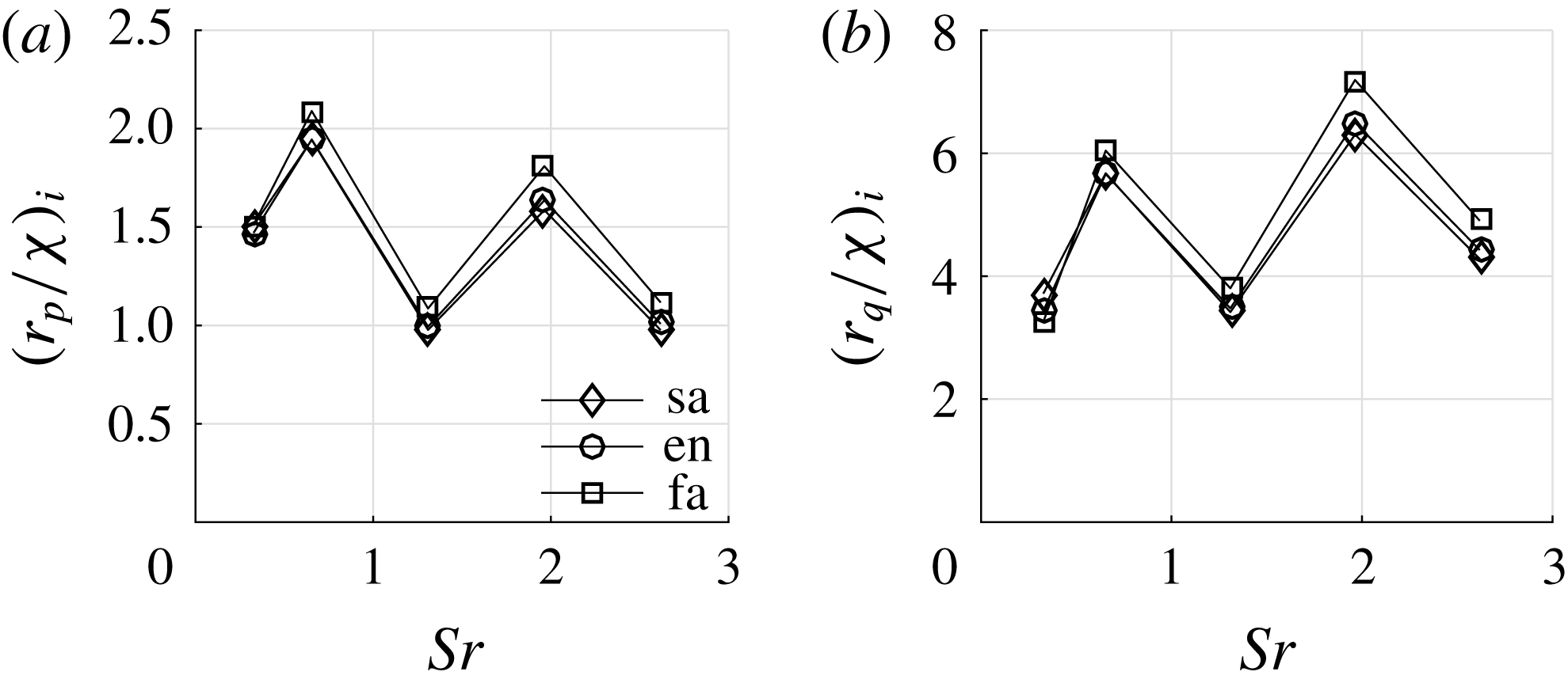
where the upper sign in (4.18) is valid for the fast acoustic mode and the lower sign denotes the slow acoustic mode. Chaudhry & Candler found the pressure response coefficients of all types of incident modes to collapse when scaled by their analytic low frequency limit value. In figure 12(a) the scaled pressure response coefficients of all incident mode types at
 $Re=109\,375$
are plotted against the Strouhal number. Since the frequencies of this investigation were chosen according to the resonant behaviour of the larger SPP, the trend shows local minima and maxima as expected. The peak value of approximately 2 is in good agreement with the results of Chaudhry & Candler who find 2.2 when scaled to the current definition from (4.14) for a cylindrical probe. Figure 12(b) shows the heat flux response coefficients of the larger SPP. The coefficients of the different incident modes are also scaled by their analytic pressure response coefficient. The collapse of these curves using the analytic low frequency limit for pressure fluctuations also evidences the contribution of the dominant postshock acoustic wave to the heat flux fluctuations.
Frequency response to continuous incident slow acoustic (sa1_h to sa5_h), entropy (en1_h to en5_h) and fast acoustic (fa1_h to fa5_h) waves at
 $Re=109\,375$
; (a) pressure response
 $r_{p}$
scaled by the analytic low frequency limit of the pressure response
 $\unicode[STIX]{x1D712}_{i}$
,
 $i$
being as, en or af; (b) heat flux response
 $r_{q}$
scaled by the analytic low frequency limit of the pressure response
 $\unicode[STIX]{x1D712}_{i}$
,
 $i$
being sa, en or fa.

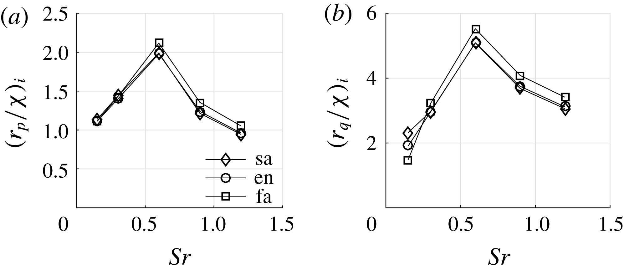
Frequency response to continuous incident slow acoustic (sa1_l to sa5_l), entropy (en1_l to en5_l) and fast acoustic (fa1_l to fa5_l) waves at
 $Re=50\,000$
; (a) pressure response
 $r_{p}$
scaled by the analytic low frequency limit of the pressure response
 $\unicode[STIX]{x1D712}_{i}$
,
 $i$
being as, en or af; (b) heat flux response
 $r_{q}$
scaled by the analytic low frequency limit of the pressure response
 $\unicode[STIX]{x1D712}_{i}$
,
 $i$
being sa, en or fa.

Figure 13(a) shows the pressure response coefficients of the smaller SPP at
 $Re=50\,000$
. As aforementioned, the Strouhal number range is limited to lower Strouhal numbers and only the first peak and valley of the response coefficients are captured in this investigation. Figure 13(b) shows the corresponding heat flux response coefficients. Again, the scaling by the analytic low frequency limit causes the curves to collapse.
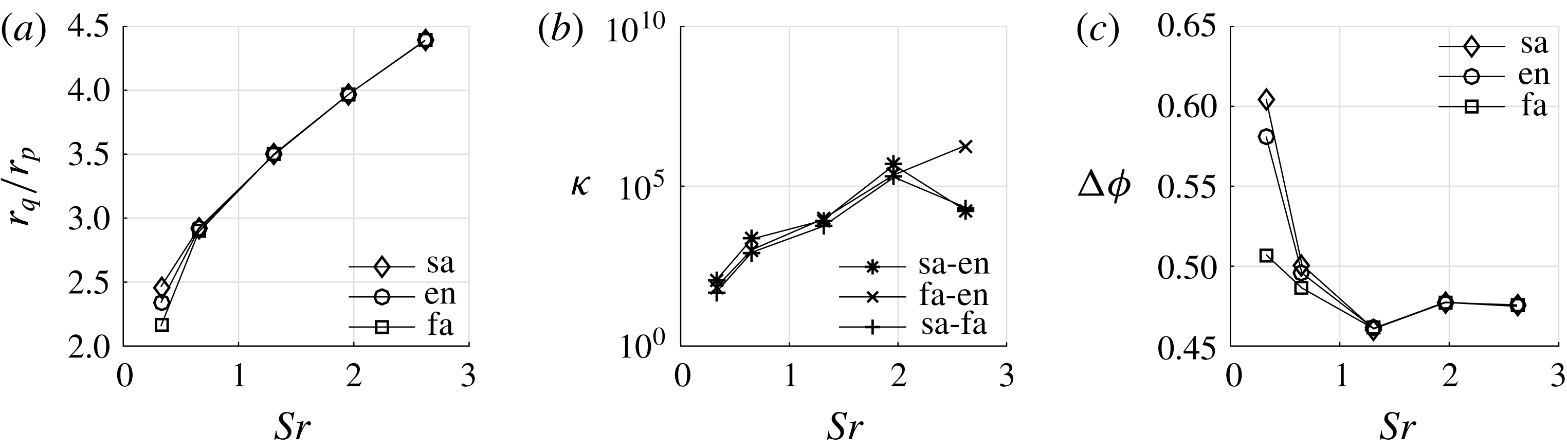
To analyse the decomposition of the pressure and heat flux fluctuation stagnation point signals into different incident modes, the ratio of the SPP heat flux and pressure response coefficients of all incident modes at
 $Re=109\,375$
is shown in figure 14(a). The ratios
 $r_{q}/r_{p}$
of all incident modes collapse starting at
 $Sr=0.655$
. Inserting the response coefficients of two types of incident modes into the transfer matrix
 $\unicode[STIX]{x1D64E}$
and calculating the condition number
 $\unicode[STIX]{x1D705}$
based on the Euclidean norm leads in figure 14(b) to high condition numbers starting at
 $Sr=0.655$
for all combinations of incident modes since the column vectors become more aligned at increasing Strouhal number. Recalling the findings of § 4.3, this can result from a diminishing initial diverging entropy wave related heat flux contribution to the heat flux response coefficient
 $r_{q}$
. Apart from the absolute value of the heat flux response coefficient
 $r_{q}$
, the diverging entropy wave related heat flux contribution could also result in a mere phase shift. Figure 14(c) shows the phase difference between the pressure and heat flux signal
 $\unicode[STIX]{x0394}\unicode[STIX]{x1D719}=\unicode[STIX]{x1D719}_{p}-\unicode[STIX]{x1D719}_{q}$
of all incident modes versus the Strouhal number. At
 $Sr=0.655$
a difference between the initial modes is still visible, even though the ratio of the response coefficient collapse. The influence of the initial diverging entropy wave related heat flux contribution to the heat flux absolute value and phase vanishes between
 $Sr=0.655$
and
 $Sr=1.309$
. This agrees well with the a priori determined value of
 $Sr_{D,co}=1$
in § 4.4.
Analysis of the decomposition of the pressure and heat flux fluctuation signals at
 $Re=109\,375$
; (a) ratio of heat flux and pressure response
 $r_{q}/r_{p}$
versus the Strouhal number of the continuous incident waves; (b) condition number
 $\unicode[STIX]{x1D705}$
of the transfer matrix
 $\unicode[STIX]{x1D64E}$
using the Euclidean norm for all combinations of incident modes; (c) phase difference between the pressure and heat flux signal
 $\unicode[STIX]{x0394}\unicode[STIX]{x1D719}=\unicode[STIX]{x1D719}_{p}-\unicode[STIX]{x1D719}_{q}$
.

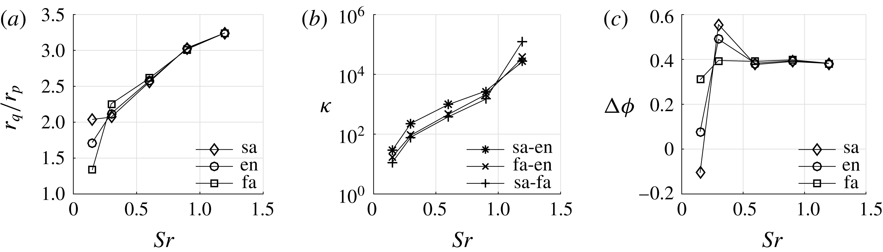
An analogous analysis can be conducted for the smaller SPP at
 $Re=50\,000$
. The corresponding data are shown in figure 15. For the lower Reynolds number case, the diverging entropy wave related heat flux contribution disappears in the response coefficient ratio and phase difference between
 $Sr=0.6$
and
 $Sr=0.9$
. This again matches well with the a priori determined value of
 $Sr_{D,co}=0.7$
.
Analysis of the decomposition of the pressure and heat flux fluctuation signals at
 $Re=50\,000$
; (a) ratio of heat flux and pressure response
 $r_{q}/r_{p}$
versus the Strouhal number of the continuous incident waves; (b) condition number
 $\unicode[STIX]{x1D705}$
of the transfer matrix
 $\unicode[STIX]{x1D64E}$
using the Euclidean norm for all combinations of incident modes; (c) phase difference between the pressure and heat flux signal
 $\unicode[STIX]{x0394}\unicode[STIX]{x1D719}=\unicode[STIX]{x1D719}_{p}-\unicode[STIX]{x1D719}_{q}$
.

5 Conclusion
To determine the wind tunnel noise in supersonic test facilities, a new modal decomposition method based on pressure and heat flux fluctuation measurements and a numerically determined transfer matrix was presented in Schilden et al. (Reference Schilden, Schröder, Ali, Wu, Schreyer and Radespiel2016). For this new method, the properties of the ‘rounded’ SPP configuration from Ali et al. (Reference Ali, Zárate Cárdenas, Radespiel, Schilden and Schröder2018) are evaluated at two Reynolds numbers in this study. The proposed method assumes tunnel noise to consist of entropy and acoustic waves that prior to being perceived by pressure or heat flux transducers are modulated by the shock wave occurring upstream of the probe. Pressure and heat flux fluctuations at the transducer position highly depend on the wave pattern in the subsonic region between shock wave and probe. To determine the properties of SPPs for the modal decomposition method, this wave pattern and the mechanism of how these waves generate pressure and heat flux fluctuations were analysed.
First, the unperturbed flow around the SPP was validated and analysed. From the flow field downstream of the shock wave the time scales of acoustic and entropy disturbances propagating between shock and SPP could be obtained. The non-dimensional standoff Strouhal number which describes the interference of acoustic waves is
 $Sr_{ac}=1.274$
for the lower Reynolds number. The Reynolds number effect is below 1 %. The time scale of the entropy wave is one order of magnitude larger than its acoustic counterpart.
Next, the impact of single pulses of acoustic and entropy waves onto the SPP was investigated. All incident modes lead to initial diverging acoustic and entropy waves with different ratios of magnitudes. The postshock disturbance compositions differ and the necessary condition for a decomposition is fulfilled. The postshock acoustic wave oscillates in the subsonic region between shock wave and SPP, while the initial diverging entropy wave convects with the flow. When the oscillating acoustic wave is reflected at the shock wave, further entropy waves are generated. The stagnation point pressure time series showed an insignificant postshock entropy wave response in comparison to the postshock acoustic wave related pressure signal. On the other hand, the heat flux is determined by the postshock acoustic wave and the postshock entropy waves, where the entropy wave response is an order of magnitude lower. Thus, the observation of Ali et al. (Reference Ali, Zárate Cárdenas, Radespiel, Schilden and Schröder2018), i.e. constructive interference in the heat flux data, is fundamentally described. The generation of heat flux fluctuations by acoustic waves could be linked to the generation of entropy spots very close to the wall. This mechanism is a direct consequence of the isothermal wall boundary condition. The influence of thermal inertia on the transfer function remains to be evaluated.
Based on the time scales obtained from the unperturbed flow and the observations of the interaction of single pulses of incident disturbance modes with the shock wave and the SPP, a model equation for the stagnation point pressure and heat flux fluctuations was formulated to describe and analyse the superposition of the postshock waves. The postshock acoustic and entropy waves were shown to interfere constructively at Strouhal numbers satisfying
 $Sr=(0.5+n)Sr_{ac}$
with
 $n\in \mathbb{N}$
. Destructive interference occurs at integer multiples of
 $Sr_{ac}$
. Rearranging the model equation for the stagnation point heat flux fluctuations, the postshock acoustic waves were shown to have a twofold contribution to the signal. First, they directly cause a heat flux during their reflection at the wall. Second, the heat flux caused by the reflection generated entropy waves must be attributed to the postshock acoustic waves. Therefore, the initial diverging entropy wave must be measured by the heat flux sensor to differentiate between incident mode types.
Since the recording of the initial diverging entropy wave is of fundamental importance for the modal decomposition method, the transfer function between postshock entropy waves and heat flux was analysed by control theory. Two approaches for the generation of a step response were presented. First, the domain was flooded with an entropy wave. Second, a converged simulation was restarted with a slightly altered Reynolds number. The later approach showed the advantage of changing the local Reynolds number, as a sudden change of entropy would do, without generating an additional strong heat flux response to postshock acoustic waves during the convergence to a new pressure field. The results of this analysis showed that the stagnation point heat flux step response is of low pass filter type. Its cutoff Strouhal number could be estimated from the step response to be approximately 0.7 for the lower Reynolds number and about 1 for the higher Reynolds number. As a consequence, the postshock entropy waves that are caused by tunnel noise at Strouhal numbers higher than the cutoff Strouhal number can not be perceived by the transducer.
Finally, the frequency response to continuous incident disturbance modes was computed and response coefficients of the transfer matrix were determined. The pressure response showed the resonant behaviour according to the findings of Chaudhry & Candler (Reference Chaudhry and Candler2016) and experiments by Ali et al. (Reference Ali, Zárate Cárdenas, Radespiel, Schilden and Schröder2018). Furthermore, also the heat flux response interfered according to the time scale of the postshock acoustic wave which was also found in the results of Ali et al. (Reference Ali, Zárate Cárdenas, Radespiel, Schilden and Schröder2018). The ratio of the pressure and heat flux response coefficients for all types of incident disturbance modes converge in a frequency range higher than the cutoff Strouhal number. The same holds for the phase difference between the pressure and heat flux signal. As expected, above the cutoff Strouhal number all incident disturbance modes lead to linearly dependent pressure and heat flux signals. Although the components of tunnel noise, i.e. the acoustic and entropy mode, can be measured at all Strouhal numbers with pressure and heat flux probes, at Strouhal numbers higher than the cutoff Strouhal number for postshock entropy waves only the postshock acoustic part of the tunnel noise can be perceived by the probes. The proposed modal decomposition method that relies on the measurement of postshock entropy waves is destined to fail if the experimental input data lack this information. In brief, the application of SPPs in the scope of the new modal decomposition method is, as for most measuring techniques, restricted to Strouhal numbers below the cutoff Strouhal number. That is, the size of the probe is extremely important.
In the present work, the Strouhal number restriction for a rounded cylinder shaped probe at two Reynolds numbers and
 $Ma=5.9$
for a new modal decomposition method was analysed. It was shown how to predict the flow related restrictions by generating a step response in the numerical simulations and applying control theory to it. The discussion that led to our approaches for generating a step response is specific to our problem but the idea, i.e. to somehow generate a real step response, is valuable. Every researcher developing transducers for a specific purpose or using well known sensors beyond their scope benefits from knowing the type of transfer function to expect in the application. It was shown how numerical simulations can be helpful for that purpose.
Acknowledgements
This work has been funded by the German Research Foundation (DFG) within the HYPTRANS PAK742. The support is gratefully acknowledged. Computing resources were provided by the High Performance Computing Center Stuttgart (HLRS) and the Jülich Supercomputing Center.