1 Introduction
The interaction of oceanic currents with spatially variable topography represents one of the most fundamental and challenging problems in geophysical fluid dynamics (e.g. Treguier & McWilliams Reference Treguier and McWilliams1990; Treguier & Panetta Reference Treguier and Panetta1994; Holloway Reference Holloway2008). There is overwhelming evidence that the non-uniformity of the ocean depth has major consequences for the intensity and pattern of flows at various scales (e.g. Holloway Reference Holloway1986; Dewar Reference Dewar1998; Thompson Reference Thompson2010; Thompson & Sallée Reference Thompson and Sallée2012; LaCasce et al. Reference LaCasce, Escartin, Chassignet and Xu2019). However, the physical mechanisms of such interactions have only been partially explained after more than half a century of investigation. Particularly relevant for our study is the observation that topography can dramatically alter properties of baroclinic instability (e.g. Hart Reference Hart1975; Vallis & Maltrud Reference Vallis and Maltrud1993; Chen, Kamenkovich & Berloff Reference Chen, Kamenkovich and Berloff2015) which, in turn, is a major source of mesoscale variability in the ocean (e.g. Pedlosky Reference Pedlosky1987; Vallis Reference Vallis2006; Marshall, Maddison & Berloff Reference Marshall, Maddison and Berloff2012). The term mesoscale variability is used here to describe eddies of the lateral extent of the order of 100 km, which dominate transient flow components in much of the World Ocean (e.g. Stammer Reference Stammer1998; Chelton et al. Reference Chelton, Schlax, Samelson and de Szoeke2007). Mesoscale eddies profoundly affect large-scale circulation (e.g. Robinson Reference Robinson1983; Olson Reference Olson1991; McWilliams Reference McWilliams2008), particularly in the Southern Ocean (e.g. Marshall & Radko Reference Marshall and Radko2003). They are known to influence oceanic heat budget (e.g. Griffies et al. Reference Griffies, Winton, Anderson, Benson, Delworth, Dufour, Dunne, Goddard, Morrison and Rosati2015), biological productivity (e.g. McGillicuddy Reference McGillicuddy2016) and dispersion of pollutants (e.g. Masumoto et al. Reference Masumoto, Miyazawa, Tsumune, Tsubono, Kobayashi, Kawamura, Estournel, Marsaleix, Lanerolle and Mehra2012). The ubiquity and geophysical significance of mesoscale eddies demand clear physical insight into all aspects of their dynamics. From a more pragmatic perspective, it is also critical to develop parameterizations of small-scale processes that affect baroclinic instability but are not fully resolved by the current generation of global numerical models.
While the effects of topography on baroclinic instability and on ensuing eddies have already been addressed in a number of studies, this research area has been disproportionately dominated by models in which scales of topography are commensurate with or exceed those of mesoscale variability (e.g. Chen & Kamenkovich Reference Chen and Kamenkovich2013; Radko & Kamenkovich Reference Radko and Kamenkovich2017; Brown, Gulliver & Radko Reference Brown, Gulliver and Radko2019). The impact of submesoscale topography – defined here as structures with a lateral extent of 1–10 km – has been much less investigated. Notable exceptions include analytical models of Benilov (Reference Benilov2001) and Vanneste (Reference Vanneste2003), which quantified linear stability properties of large-scale vertically sheared currents. These studies suggest that submesoscale topography can have a strong and adverse influence on the development of baroclinic instability. The possibility of submesoscale stabilization is also supported by recent numerical simulations of LaCasce et al. (Reference LaCasce, Escartin, Chassignet and Xu2019), who demonstrated that topographic features of realistic height can effectively suppress the baroclinic instability of currents that are comparable in size and strength to the Gulf Stream and Kuroshio. Yet another compelling argument that underscores the potential significance of submesoscale topography comes from the inspection of observationally derived bathymetric spectra. This analysis (appendix A) shows that the variance of the bottom slope is dominated by submesoscale components of topography. Of course, this observation by itself does not guarantee that its impact on baroclinic instability exceeds the influence of large-scale topography. For instance, it is known that small-scale modes induced by the bottom roughness tend to decay rapidly in the vertical direction (Callies Reference Callies2018). Nevertheless, the estimates in appendix A motivate efforts to explore the impact of submesoscale topography on baroclinic instability in greater detail.
The present investigation into topographically induced effects represents a component of the broader inquiry into the dynamics of the submesoscale variability of oceanic flows – a topic which has recently drawn much attention from the oceanographic community (e.g. McWilliams Reference McWilliams2016). This interest was fuelled by advances in observational techniques and computing power, which led to a broader appreciation of the significance of submesoscale structures and concurrently opened previously inaccessible avenues for their exploration (e.g. Levy et al. Reference Levy, Klein, Treguier, Iovino, Madec, Masson and Takahashi2010; Chassignet & Xu Reference Chassignet and Xu2017). One of the potentially critical consequences of submesoscale variability is related to energy transfer between different circulation components. Mechanical and thermodynamic forcing of the ocean occurs on the scale of its basins, whereas the energy is ultimately dissipated by molecular processes acting on the microscale. Unlike larger structures, submesoscale eddies may not fully support the inverse energy cascade – which is expected for two-dimensional turbulence – resulting in energy leakage to both larger and smaller scales (e.g. Thomas, Tandon & Mahadevan Reference Thomas, Tandon, Mahadevan, Hecht and Hasumi2008; Nikurashin, Vallis & Adcroft Reference Nikurashin, Vallis and Adcroft2013). Thus, submesoscale variability could represent an essential conduit for energy transfer to the microscale.
While high-resolution simulations clearly reflect the general ubiquity of submesoscales, the intensity of these structures is spatially heterogeneous. In particular, submesoscale eddies are known to be very active in the upper mixed layer (e.g. Fox-Kemper, Ferrari & Hallberg Reference Fox-Kemper, Ferrari and Hallberg2008; Whitt & Taylor Reference Whitt and Taylor2017) and in the vicinity of salient topographic features (e.g. Dewar, McWilliams & Molemaker Reference Dewar, McWilliams and Molemaker2015; Rosso et al. Reference Rosso, Hogg, Kiss and Gayen2015; Gula, Molemaker & McWilliams Reference Gula, Molemaker and McWilliams2016). The present investigation is focused on the dynamics of latter, topographically induced submesoscale variability, which is examined using a multi-layer ocean model of variable depth. The background current in our model is baroclinically unstable and therefore the flow field is heavily populated by mesoscale eddies. The model topography contains submesoscale features and their interaction with baroclinic instability produces an active submesoscale eddy field which, in turn, affects mesoscale structures. We find, in accord with previous studies, that dominant topographically induced submesoscale patterns are largely contained in the lowest density layer that is in direct contact with the sea floor. Nevertheless, the influence of these submesoscale patterns can be surprisingly non-local, extending vertically throughout the entire water column and reducing the intensity of baroclinic instability at all levels.
The analysis of the interaction between submesoscale topography and eddies generated by baroclinic instability is accomplished using a multiscale method. Multiscale modelling is a vibrant, rapidly developing field with a broad range of applications described, for example, in the review by Mei & Vernescu (Reference Mei and Vernescu2010). Multiscale methods involve rewriting governing equations using two distinct sets of independent spatial variables corresponding to small and large scales, which ultimately leads to a set of evolutionary equations expressed entirely in terms of large-scale quantities. The analysis is based on the expansion in powers of a small parameter
 $(\unicode[STIX]{x1D700})$
representing the ratio of typical scales of the small-scale pattern (submesoscale variability in our case) and those of larger structures (mesoscale eddies). Since multiscale methods are based directly on governing equations, they do not depend on empirical parameterizations required by other analytical models.
The majority of multiscale models consider steady analytical small-scale patterns, exemplified by the Kolmogorov model (e.g. Meshalkin & Sinai Reference Meshalkin and Sinai1961; Manfroi & Young Reference Manfroi and Young1999, Reference Manfroi and Young2002; Balmforth & Young Reference Balmforth and Young2002, Reference Balmforth and Young2005; Radko Reference Radko2014) which represents the background fields by a single Fourier harmonic. Such studies have been generalized to incorporate more complicated two-dimensional small-scale structures (e.g. Gama, Vergassola & Frisch Reference Gama, Vergassola and Frisch1994; Vanneste Reference Vanneste2000; Novikov & Papanicolaou Reference Novikov and Papanicolaou2001; Radko Reference Radko2011). Analogous models have also been developed for three-dimensional patterns (e.g. Dubrulle & Frisch Reference Dubrulle and Frisch1991; Wirth, Gama & Frisch Reference Wirth, Gama and Frisch1995). A series of recent studies (Radko Reference Radko2016, Reference Radko2019; Radko & Kamenkovich Reference Radko and Kamenkovich2017) has shown that techniques of multiscale analysis can also be successfully applied to realistic, dynamically consistent flow fields. Such models offer a quantitative description of cross-scale interactions that could be tested by observations and comprehensive simulations. At the same time, they retain the dynamic transparency of analytical multiscale solutions, making it possible to unambiguously identify the entire chain of physical processes at work. The present investigation utilizes the multiscale framework to explain the interplay of mesoscale eddies, submesoscale variability and topographic influences. We consider an idealized harmonic model of bathymetry, which leads to transparent Kolmogorov-type solutions. However, it is our belief that the proposed model can be generalized to incorporate more general patterns of topography, such as based on regional in situ observations or on statistical bathymetric spectra (e.g. Goff & Jordan Reference Goff and Jordan1988).
In addition to the general oceanographic interest in explaining the dynamics of interaction between mesoscale eddies and submesoscale topography from first principles, multiscale modelling also opens an opportunity to develop accurate and physically motivated submesoscale parameterizations. Despite continuous advances in high-performance computing, it is highly unlikely that submesoscale-resolving models will become a standard choice for extended climate simulations in the foreseeable future. Thus, the development of submesoscale parameterizations may represent one of the current priorities in climate science and global ocean modelling. Finally, this study makes it possible to assess the performance characteristics of the multiscale model itself. Since the model formally assumes asymptotic scale separation between interacting flow components, the question arises as to whether it retains its capabilities when the lines between large and small scales are blurred – which is indeed the case for the problem of mesoscale–submesoscale interaction. This issue is addressed by comparing the asymptotic and fully nonlinear solutions in a relatively simple and easily controlled system. The results of this analysis are encouraging; we find that the multiscale method is surprisingly accurate even when the scale separation is virtually non-existent.
The material is organized as follows. In § 2, we describe the model configuration and present illustrative numerical examples of active interaction between mesoscale variability and topographically induced submesoscales. The multiscale theory representing this interaction is formulated in § 3. The model predictions are then discussed and compared to their nonlinear counterparts (§ 4). In § 5, we draw conclusions and summarize our findings. The estimates of the relevant scales of submesoscale topography from observationally derived bathymetric spectra are given in appendix A. Most calculations in this study, analytical and numerical, are based on the quasi-geostrophic model. Therefore, in order to assess the potential significance of non-quasi-geostrophic effects, we also present (appendix B) a series of simulations performed with a more general shallow-water model. Both models behave in a consistent manner, which validates conclusions based on the quasi-geostrophic framework for the regime of interest.
2 Preliminary simulations
Consider a baroclinically unstable zonal flow in an
 $n$
-layer ocean on the beta plane (figure 1). The basic current is assumed to be laterally homogeneous and steady – the configuration which is maintained indefinitely by the mechanical and thermodynamic forcing of the system. In the following model,
 $U_{i}^{\ast }$
,
 $H_{i}^{\ast }$
and
 $\unicode[STIX]{x1D70C}_{i}^{\ast }$
represent the basic speed, depth and density of layer
 $i$
, where
 $i=1,\ldots ,n$
, and the asterisks denote dimensional quantities. The basic velocity of the lowest layer
 $n$
, which is in the direct contact with the sea floor, is assumed to be zero (
 $U_{n}^{\ast }=0$
). Theoretical development is simplified by assuming identical density differences between adjacent layers
 $\unicode[STIX]{x0394}\unicode[STIX]{x1D70C}^{\ast }=\unicode[STIX]{x1D70C}_{i}^{\ast }-\unicode[STIX]{x1D70C}_{i-1}^{\ast }$
, although the generalization to variable
 $\unicode[STIX]{x0394}\unicode[STIX]{x1D70C}$
would be rather straightforward. Baroclinic instability of the basic state generates active mesoscale variability, which is dominated by eddies with scales comparable to the radius of deformation. To be specific, in the following analysis we shall refer to the radius of deformation based on the entire ocean depth
 $H^{\ast }=\sum _{i=1}^{n}H_{i}^{\ast }$
,
 $$\begin{eqnarray}R_{d}^{\ast }\equiv \frac{\sqrt{g^{\prime \ast }H^{\ast }}}{f_{0}^{\ast }},\end{eqnarray}$$
where
 $$\begin{eqnarray}g^{\prime \ast }=g\frac{\unicode[STIX]{x1D70C}_{n}^{\ast }-\unicode[STIX]{x1D70C}_{1}^{\ast }}{\unicode[STIX]{x1D70C}_{0}^{\ast }}=g\frac{\unicode[STIX]{x0394}\unicode[STIX]{x1D70C}^{\ast }}{\unicode[STIX]{x1D70C}_{0}^{\ast }}(n-1)\end{eqnarray}$$
is the reduced gravity,
 $\unicode[STIX]{x1D70C}_{0}^{\ast }$
is the reference density,
 $f_{0}^{\ast }$
is the reference value of the Coriolis parameter (
 $f^{\ast }$
) in the beta-plane approximation.
Schematic diagram illustrating the interaction of mesoscale variability with submesoscale topographic features.

As indicated in figure 1, the model topography is spatially variable on scales
 $(L_{topogr}^{\ast })$
that are less than the radius of deformation,
 $$\begin{eqnarray}L_{topogr}^{\ast }\sim \unicode[STIX]{x1D700}R_{d}^{\ast },\end{eqnarray}$$
where
 $\unicode[STIX]{x1D700}\ll 1$
. Baroclinic instability of the basic flow generates active mesoscale variability in all layers. The interaction of eddies in the lower layer with uneven sea floor produces circulation patterns that are commensurate in size with the scale of topographic variability. The dynamics of these submesoscale structures
 $({\sim}L_{topogr}^{\ast })$
and their interaction with larger mesoscale eddies
 $({\sim}R_{d}^{\ast })$
are the main subjects of our investigation.
In this study, we shall focus on the intermediate range of topographic scales that lead to geostrophically balanced submesoscale variability. These scales satisfy the double requirement
 $$\begin{eqnarray}\frac{U^{\ast }}{f_{0}^{\ast }}\ll L_{topogr}^{\ast }\ll R_{d}^{\ast },\end{eqnarray}$$
where
 $U^{\ast }=\max _{i}(|U_{i}^{\ast }|)$
. Restricting the following analysis to the upper-submesoscale range (2.4) obviously limits the breadth of physical effects that the model can possibly represent. For instance, the forward energy cascade by submesoscales is left outside of the scope of the present investigation. Nevertheless, it is generally accepted (e.g. McWilliams Reference McWilliams2016) that the exploration of balanced submesoscale dynamics represents a convenient starting point of analysis, particularly for the purpose of developing and testing new theoretical models. Furthermore, the comparison of the following quasi-geostrophic solutions with their counterparts generated using a more general shallow-water model (appendix B) reveals their qualitative consistency. The inequality (2.4) is satisfied by relatively slow flows in the interior of ocean basins. For instance, assuming
 $U^{\ast }\sim 3\times 10^{-2}~\text{m}~\text{s}^{-1}$
,
 $R_{d}^{\ast }\sim 6\times 10^{4}~\text{m}$
,
 $f_{0}^{\ast }\sim 10^{-4}~\text{s}^{-1}$
and
 $L_{topogr}^{\ast }\sim 3\times 10^{3}~\text{m}$
, we arrive at
 $$\begin{eqnarray}Ro=\frac{U^{\ast }}{f_{0}^{\ast }L_{topogr}^{\ast }}\sim 0.1,\quad \unicode[STIX]{x1D700}=\frac{L_{topogr}^{\ast }}{R_{d}^{\ast }}\sim 0.05.\end{eqnarray}$$
The low values of the Rossby number (
 $Ro$
) and the scale separation parameter (
 $\unicode[STIX]{x1D700}$
) justify the concurrent application of the multiscale method (§ 3) and the more common quasi-geostrophic model (e.g. Charney Reference Charney1948, Reference Charney1971; Pedlosky Reference Pedlosky1987):
 $$\begin{eqnarray}\left.\begin{array}{@{}c@{}}\displaystyle \frac{\unicode[STIX]{x2202}Q_{1}^{\ast }}{\unicode[STIX]{x2202}t^{\ast }}+J(\unicode[STIX]{x1D6F9}_{1}^{\ast },Q_{1}^{\ast })=\unicode[STIX]{x1D708}^{\ast }\unicode[STIX]{x1D6FB}^{4}\unicode[STIX]{x1D6F9}_{1}^{\ast },\\ \displaystyle Q_{1}^{\ast }=\unicode[STIX]{x1D6FB}^{2}\unicode[STIX]{x1D6F9}_{1}^{\ast }+\frac{f_{0}^{\ast 2}}{g_{loc}^{\prime \ast }H_{1}^{\ast }}(\unicode[STIX]{x1D6F9}_{2}^{\ast }-\unicode[STIX]{x1D6F9}_{1}^{\ast })+\unicode[STIX]{x1D6FD}^{\ast }y^{\ast },\\ \displaystyle \frac{\unicode[STIX]{x2202}Q_{i}^{\ast }}{\unicode[STIX]{x2202}t^{\ast }}+J(\unicode[STIX]{x1D6F9}_{i}^{\ast },Q_{i}^{\ast })=\unicode[STIX]{x1D708}^{\ast }\unicode[STIX]{x1D6FB}^{4}\unicode[STIX]{x1D6F9}_{i}^{\ast },\quad i=2,\ldots ,(n-1),\\ \displaystyle Q_{i}^{\ast }=\unicode[STIX]{x1D6FB}^{2}\unicode[STIX]{x1D6F9}_{i}^{\ast }+\frac{f_{0}^{\ast 2}}{g_{loc}^{\prime \ast }H_{i}^{\ast }}(\unicode[STIX]{x1D6F9}_{i-1}^{\ast }+\unicode[STIX]{x1D6F9}_{i+1}^{\ast }-2\unicode[STIX]{x1D6F9}_{i}^{\ast })+\unicode[STIX]{x1D6FD}^{\ast }y^{\ast },\\ \displaystyle \frac{\unicode[STIX]{x2202}Q_{n}^{\ast }}{\unicode[STIX]{x2202}t^{\ast }}+J(\unicode[STIX]{x1D6F9}_{n}^{\ast },Q_{n}^{\ast })=\unicode[STIX]{x1D708}^{\ast }\unicode[STIX]{x1D6FB}^{4}\unicode[STIX]{x1D6F9}_{n}^{\ast }-\unicode[STIX]{x1D6FE}^{\ast }\unicode[STIX]{x1D6FB}^{2}\unicode[STIX]{x1D6F9}_{n}^{\ast },\\ \displaystyle Q_{n}^{\ast }=\unicode[STIX]{x1D6FB}^{2}\unicode[STIX]{x1D6F9}_{n}^{\ast }+\frac{f_{0}^{\ast 2}}{g_{loc}^{\prime \ast }H_{n}^{\ast }}(\unicode[STIX]{x1D6F9}_{n-1}^{\ast }-\unicode[STIX]{x1D6F9}_{n}^{\ast })+\unicode[STIX]{x1D6FD}^{\ast }y^{\ast }+f_{0}^{\ast }\frac{\unicode[STIX]{x1D702}_{b}^{\ast }}{H_{n}^{\ast }},\end{array}\right\}\end{eqnarray}$$
where
 $\unicode[STIX]{x1D6F9}_{i}^{\ast }$
and
 $Q_{i}^{\ast }$
are the streamfunction and potential vorticity (PV) in layer
 $i$
,
 $g_{loc}^{\prime \ast }=g\unicode[STIX]{x0394}\unicode[STIX]{x1D70C}^{\ast }/\unicode[STIX]{x1D70C}_{0}^{\ast }=g^{\prime \ast }/(n-1)$
,
 $\unicode[STIX]{x1D6FD}^{\ast }=\unicode[STIX]{x2202}f^{\ast }/\unicode[STIX]{x2202}y^{\ast }=\text{const.}$
,
 $\unicode[STIX]{x1D708}^{\ast }$
is the lateral viscosity,
 $\unicode[STIX]{x1D6FE}^{\ast }$
is the bottom drag coefficient and
 $\unicode[STIX]{x1D702}_{b}^{\ast }$
is the variation of the total ocean depth relative to its mean value. The total lateral velocities in each layer are separated into the background components
 $(U_{i}^{\ast },0)$
and perturbations
 $(u_{i}^{\ast },v_{i}^{\ast })$
. These velocity fields are readily expressed in terms of the streamfunction:
 $(U_{i}^{\ast }+u_{i}^{\ast },v_{i}^{\ast })=(-\unicode[STIX]{x2202}\unicode[STIX]{x1D6F9}_{i}^{\ast }/\unicode[STIX]{x2202}y,\unicode[STIX]{x2202}\unicode[STIX]{x1D6F9}_{i}^{\ast }/\unicode[STIX]{x2202}x)$
. The net streamfunction in each layer
 $(\unicode[STIX]{x1D6F9}_{i}^{\ast })$
is also separated into the basic state representing the background steady current
 $(-U_{i}^{\ast }y^{\ast })$
and the perturbation
 $(\unicode[STIX]{x1D713}_{i}^{\ast })$
. To be specific, in this study we consider the eastward sub-surface flow
 $(U_{1}^{\ast }>0)$
in the Northern hemisphere
 $(f^{\ast }>0)$
. However, the following analysis can be readily reproduced for
 $f^{\ast }<0$
and/or
 $U_{1}^{\ast }<0$
.
When governing equations (2.6) are expressed in terms of perturbations
 $\unicode[STIX]{x1D713}_{i}^{\ast }$
, we arrive at
 $$\begin{eqnarray}\left.\begin{array}{@{}c@{}}\displaystyle \frac{\unicode[STIX]{x2202}q_{1}^{\ast }}{\unicode[STIX]{x2202}t^{\ast }}+J(\unicode[STIX]{x1D713}_{1}^{\ast },q_{1}^{\ast })+\unicode[STIX]{x1D6FD}^{\ast }\frac{\unicode[STIX]{x2202}\unicode[STIX]{x1D713}_{1}^{\ast }}{\unicode[STIX]{x2202}x^{\ast }}+\frac{f_{0}^{\ast 2}(U_{1}^{\ast }-U_{2}^{\ast })}{g_{loc}^{\prime \ast }H_{1}^{\ast }}\frac{\unicode[STIX]{x2202}\unicode[STIX]{x1D713}_{1}^{\ast }}{\unicode[STIX]{x2202}x^{\ast }}+U_{1}^{\ast }\frac{\unicode[STIX]{x2202}q_{1}^{\ast }}{\unicode[STIX]{x2202}x^{\ast }}=\unicode[STIX]{x1D708}^{\ast }\unicode[STIX]{x1D6FB}^{4}\unicode[STIX]{x1D713}_{1}^{\ast },\\ \displaystyle \begin{array}{@{}l@{}}\displaystyle \frac{\unicode[STIX]{x2202}q_{i}^{\ast }}{\unicode[STIX]{x2202}t^{\ast }}+J(\unicode[STIX]{x1D713}_{i}^{\ast },q_{i}^{\ast })+\unicode[STIX]{x1D6FD}^{\ast }\frac{\unicode[STIX]{x2202}\unicode[STIX]{x1D713}_{1}^{\ast }}{\unicode[STIX]{x2202}x^{\ast }}+\frac{f_{0}^{\ast 2}(2U_{i}^{\ast }-U_{i-1}^{\ast }-U_{i+1}^{\ast })}{g_{loc}^{\prime \ast }H_{i}^{\ast }}\frac{\unicode[STIX]{x2202}\unicode[STIX]{x1D713}_{1}^{\ast }}{\unicode[STIX]{x2202}x^{\ast }}\\ \quad +\,\displaystyle U_{i}^{\ast }\frac{\unicode[STIX]{x2202}q_{i}^{\ast }}{\unicode[STIX]{x2202}x^{\ast }}=\unicode[STIX]{x1D708}^{\ast }\unicode[STIX]{x1D6FB}^{4}\unicode[STIX]{x1D713}_{1}^{\ast },\quad i=2,\ldots ,(n-1),\end{array}\\ \displaystyle \frac{\unicode[STIX]{x2202}q_{n}^{\ast }}{\unicode[STIX]{x2202}t^{\ast }}+J(\unicode[STIX]{x1D713}_{n}^{\ast },q_{n}^{\ast })+\unicode[STIX]{x1D6FD}^{\ast }\frac{\unicode[STIX]{x2202}\unicode[STIX]{x1D713}_{n}^{\ast }}{\unicode[STIX]{x2202}x^{\ast }}-\frac{f_{0}^{\ast 2}U_{n-1}^{\ast }}{g_{loc}^{\prime \ast }H_{n}^{\ast }}\frac{\unicode[STIX]{x2202}\unicode[STIX]{x1D713}_{n}^{\ast }}{\unicode[STIX]{x2202}x^{\ast }}+\frac{f_{0}^{\ast }}{H_{n}^{\ast }}J(\unicode[STIX]{x1D713}_{n}^{\ast },\unicode[STIX]{x1D702}_{b}^{\ast })=\unicode[STIX]{x1D708}^{\ast }\unicode[STIX]{x1D6FB}^{4}\unicode[STIX]{x1D713}_{n}^{\ast }-\unicode[STIX]{x1D6FE}^{\ast }\unicode[STIX]{x1D6FB}^{2}\unicode[STIX]{x1D713}_{n}^{\ast },\end{array}\right\}\end{eqnarray}$$
where
 $q_{i}^{\ast }$
are the perturbation PV fields,
 $$\begin{eqnarray}\left.\begin{array}{@{}c@{}}\displaystyle q_{1}^{\ast }=\unicode[STIX]{x1D6FB}^{2}\unicode[STIX]{x1D713}_{1}^{\ast }+\frac{f_{0}^{\ast 2}}{g_{loc}^{\prime \ast }H_{1}^{\ast }}(\unicode[STIX]{x1D713}_{2}^{\ast }-\unicode[STIX]{x1D713}_{1}^{\ast }),\\ \displaystyle q_{i}^{\ast }=\unicode[STIX]{x1D6FB}^{2}\unicode[STIX]{x1D713}_{i}^{\ast }+\frac{f_{0}^{\ast 2}}{g_{loc}^{\prime \ast }H_{i}^{\ast }}(\unicode[STIX]{x1D713}_{i+1}^{\ast }+\unicode[STIX]{x1D713}_{i-1}^{\ast }-2\unicode[STIX]{x1D713}_{i}^{\ast }),\\ \displaystyle q_{n}^{\ast }=\unicode[STIX]{x1D6FB}^{2}\unicode[STIX]{x1D713}_{n}^{\ast }+\frac{f_{0}^{\ast 2}}{g_{loc}^{\prime \ast }H_{n}^{\ast }}(\unicode[STIX]{x1D713}_{n-1}^{\ast }-\unicode[STIX]{x1D713}_{n}^{\ast }).\end{array}\quad i=2,\ldots ,(n-1),\right\}\end{eqnarray}$$
To reduce the number of controlling parameters, the governing equations (2.7) are non-dimensionalized using
 $R_{d}^{\ast }$
and
 $U_{1}^{\ast }$
as units of length and velocity respectively. The resulting non-dimensional system takes the form
 $$\begin{eqnarray}\left.\begin{array}{@{}c@{}}\displaystyle \frac{\unicode[STIX]{x2202}q_{1}}{\unicode[STIX]{x2202}t}+J(\unicode[STIX]{x1D713}_{1},q_{1})+\unicode[STIX]{x1D6FD}\frac{\unicode[STIX]{x2202}\unicode[STIX]{x1D713}_{1}}{\unicode[STIX]{x2202}x}+s_{1}(1-U_{2})\frac{\unicode[STIX]{x2202}\unicode[STIX]{x1D713}_{1}}{\unicode[STIX]{x2202}x}+\frac{\unicode[STIX]{x2202}q_{1}}{\unicode[STIX]{x2202}x}=\unicode[STIX]{x1D708}\unicode[STIX]{x1D6FB}^{4}\unicode[STIX]{x1D713}_{1},\\ \displaystyle \begin{array}{@{}l@{}}\displaystyle \frac{\unicode[STIX]{x2202}q_{i}}{\unicode[STIX]{x2202}t}+J(\unicode[STIX]{x1D713}_{i},q_{i})+\unicode[STIX]{x1D6FD}\frac{\unicode[STIX]{x2202}\unicode[STIX]{x1D713}_{i}}{\unicode[STIX]{x2202}x}+s_{i}(2U_{i}-U_{i-1}-U_{i+1})\frac{\unicode[STIX]{x2202}\unicode[STIX]{x1D713}_{i}}{\unicode[STIX]{x2202}x}\\ \displaystyle \quad +\,U_{i}\frac{\unicode[STIX]{x2202}q_{i}}{\unicode[STIX]{x2202}x}=\unicode[STIX]{x1D708}\unicode[STIX]{x1D6FB}^{4}\unicode[STIX]{x1D713}_{i},\quad i=2,\ldots ,(n-1),\end{array}\\ \displaystyle \frac{\unicode[STIX]{x2202}q_{n}}{\unicode[STIX]{x2202}t}+J(\unicode[STIX]{x1D713}_{n},q_{n})+\unicode[STIX]{x1D6FD}\frac{\unicode[STIX]{x2202}\unicode[STIX]{x1D713}_{n}}{\unicode[STIX]{x2202}x}-s_{n}U_{n-1}\frac{\unicode[STIX]{x2202}\unicode[STIX]{x1D713}_{n}}{\unicode[STIX]{x2202}x}+\frac{1}{r_{n}}J(\unicode[STIX]{x1D713}_{n},\unicode[STIX]{x1D702}_{b})=\unicode[STIX]{x1D708}\unicode[STIX]{x1D6FB}^{4}\unicode[STIX]{x1D713}_{n}-\unicode[STIX]{x1D6FE}\unicode[STIX]{x1D6FB}^{2}\unicode[STIX]{x1D713}_{n},\end{array}\right\}\end{eqnarray}$$
where
 $s_{i}=(g^{\prime \ast }H^{\ast })/(g_{loc}^{\prime }H_{i}^{\ast })=(n-1)/r_{i}$
,
 $\unicode[STIX]{x1D6FD}=(\unicode[STIX]{x1D6FD}^{\ast }R_{d}^{\ast 2})/U_{1}^{\ast }$
,
 $\unicode[STIX]{x1D708}=\unicode[STIX]{x1D708}^{\ast }/(R_{d}^{\ast }U_{1}^{\ast })$
,
 $\unicode[STIX]{x1D6FE}=(\unicode[STIX]{x1D6FE}^{\ast }R_{d}^{\ast })/U_{1}^{\ast }$
,
 $r_{i}=H_{i}^{\ast }/H^{\ast }$
are the governing parameters, and
 $\unicode[STIX]{x1D702}_{b}=(f_{0}^{\ast }R_{d}^{\ast }\unicode[STIX]{x1D702}_{b}^{\ast })/(H^{\ast }U_{1}^{\ast })$
. Note that the adopted non-dimensionalization of the topographic height implies that
 $\unicode[STIX]{x1D702}_{b}^{\ast }=\unicode[STIX]{x1D700}RoH^{\ast }\unicode[STIX]{x1D702}_{b}$
and therefore
 $O(1)$
values of
 $\unicode[STIX]{x1D702}_{b}$
considered in this study correspond to
 $\unicode[STIX]{x1D702}_{b}^{\ast }\ll H^{\ast }$
.
The non-dimensional PV perturbations reduce to
 $$\begin{eqnarray}\left.\begin{array}{@{}c@{}}q_{1}=\unicode[STIX]{x1D6FB}^{2}\unicode[STIX]{x1D713}_{1}+s_{1}(\unicode[STIX]{x1D713}_{2}-\unicode[STIX]{x1D713}_{1}),\\ q_{i}=\unicode[STIX]{x1D6FB}^{2}\unicode[STIX]{x1D713}_{i}+s_{i}(\unicode[STIX]{x1D713}_{i+1}+\unicode[STIX]{x1D713}_{i-1}-2\unicode[STIX]{x1D713}_{i}),\\ q_{n}=\unicode[STIX]{x1D6FB}^{2}\unicode[STIX]{x1D713}_{n}+s_{n}(\unicode[STIX]{x1D713}_{n-1}-\unicode[STIX]{x1D713}_{n}).\end{array}\quad i=2,\ldots ,(n-1),\right\}\end{eqnarray}$$
In the following numerical experiments, we assume doubly periodic boundary conditions for
 $\unicode[STIX]{x1D713}_{i}$
. The governing system is integrated using a dealiased pseudospectral method based on the fourth-order Runge–Kutta time-stepping scheme (e.g. Radko & Kamenkovich Reference Radko and Kamenkovich2017).
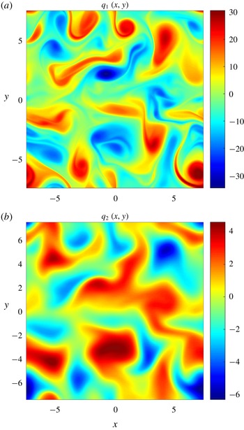
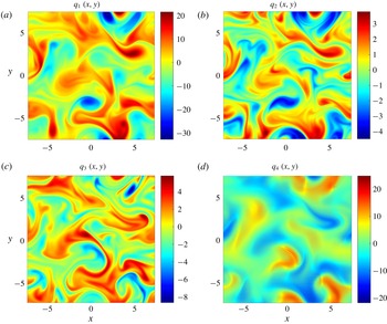
Typical patterns of PV in the upper (a) and lower (b) layers in the quasi-equilibrium phase (
 $t=500$
) of the flat-bottom simulation.

To gain preliminary insight into the interaction between baroclinic instability and submesoscale topography, we present two
 $n=2$
experiments – the flat-bottom simulation (figure 2) and its counterpart performed in an ocean of non-uniform depth (figure 3). In both cases, we use the following governing parameters:
 $$\begin{eqnarray}\unicode[STIX]{x1D6FD}=0.8,\quad \unicode[STIX]{x1D708}=0.005,\quad \unicode[STIX]{x1D6FE}=1.0,\quad r_{1}={\textstyle \frac{1}{4}},\quad r_{2}={\textstyle \frac{3}{4}},\quad L_{x}=15,\quad L_{y}=15,\end{eqnarray}$$
where
 $L_{x}$
and
 $L_{y}$
represent the zonal and meridional extents of the computational domain, which is resolved by
 $N_{x}\times N_{y}=1024\times 1024$
grid points. The model bathymetry is represented by the harmonic pattern,
 $$\begin{eqnarray}\unicode[STIX]{x1D702}_{b}=\unicode[STIX]{x1D702}_{0}\cos (kx+ly),\end{eqnarray}$$
where
 $k$
and
 $l$
are the zonal and meridional wavenumbers respectively. Adopting the idealized topography (2.12) makes it possible to express the topographic influences in terms of explicit solutions of Kolmogorov type (§ 3). The experiment in figure 3 was performed with zonally oriented bathymetry
 $(k=0)$
, a meridional wavelength of
 $d_{y}=2\unicode[STIX]{x03C0}/l=0.15$
and an amplitude of topographic variability of
 $\unicode[STIX]{x1D702}_{0}=4.5$
. Dimensionally, these parameters correspond to
 $$\begin{eqnarray}d_{y}^{\ast }=10~\text{km},\quad \unicode[STIX]{x1D702}_{0}^{\ast }=85~\text{m},\end{eqnarray}$$
where we have assumed
 $$\begin{eqnarray}\left.\begin{array}{@{}c@{}}H_{1}^{\ast }=1000~\text{m},\quad H_{2}^{\ast }=3000~\text{m},\quad U_{1}^{\ast }=0.03~\text{m}~\text{s}^{-1},\\ f_{0}^{\ast }=10^{-4}~\text{s}^{-1},\quad g^{\prime \ast }=0.01~\text{m}~\text{s}^{-1}.\end{array}\right\}\end{eqnarray}$$
The pattern (2.13) represents rather modest variations in depth and sea-floor slope, which are commonly matched or exceeded in the ocean (appendix A).
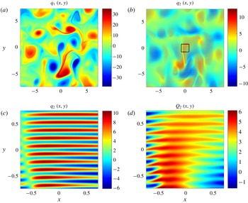
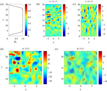
Typical patterns of PV in the upper (a) and lower (b) layers in the quasi-equilibrium phase (
 $t=500$
) of the non-uniform depth simulation. Panel (c) shows an enlarged view of the square area marked in (b) and panel (d) presents the total potential vorticity (
 $Q_{2}$
) in the same square area.

The simulations in figures 2 and 3 were initiated by the small-amplitude random distribution of
 $(\unicode[STIX]{x1D713}_{1},\unicode[STIX]{x1D713}_{2})$
– identical patterns were used for both simulations. The first evolutionary stage of each experiment is represented by the exponential growth of baroclinic instability, which is followed by its nonlinear equilibration and the transition to a statistically steady but highly disorganized regime. Figure 2(a,b) presents the typical patterns of the potential vorticity
 $(q_{1},q_{2})$
in the upper and lower layers respectively, realized during the fully developed stage of the flat-bottom simulation. While the inclusion of topography has only a moderate impact on the upper layer (figure 3
a), the lower layer PV (figure 3
b) exhibits visible modulation on small scales. Figure 3(c) shows an enlarged view of
 $q_{2}$
in the small area marked in figure 3(b), revealing a well-defined imprint of the zonally oriented topography on the lower layer. Figure 3(d) presents the pattern of the total PV in the lower layer (
 $Q_{2}$
) over the same area as shown in figure 3(c). The distribution of
 $Q_{2}$
is visibly more homogeneous over small scales than the corresponding pattern of
 $q_{2}$
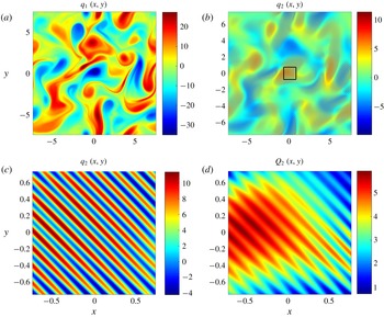
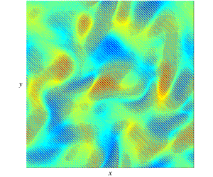
. The PV homogenization tendency will be subsequently used (§ 3) to physically interpret the stabilizing role of submesoscale topography. Figure 4 presents the analogous calculation in which bathymetric features are oriented at the angle
 $\unicode[STIX]{x1D703}=\unicode[STIX]{x03C0}/4$
relative to the zonal direction.
The same as figure 3 but for the non-zonal (
 $\unicode[STIX]{x1D703}=\unicode[STIX]{x03C0}/4$
) orientation of topography.

To be more quantitative in assessing the impact of bottom topography on the intensity and mixing characteristics of baroclinic instability, we introduce the following integral measures of the flow field. The average kinetic energy is defined as
 $$\begin{eqnarray}E_{i}=\left[\frac{u_{i}^{2}+v_{i}^{2}}{2}\right]_{xy},\quad i=1,2,\end{eqnarray}$$
where
 $(u_{i},v_{i})=(-\unicode[STIX]{x2202}\unicode[STIX]{x1D713}_{i}/\unicode[STIX]{x2202}y,\unicode[STIX]{x2202}\unicode[STIX]{x1D713}_{i}/\unicode[STIX]{x2202}x)$
are the non-dimensional perturbation velocities and the symbol
 $[\cdots \,]_{xy}$
represents averaging in
 $x$
and
 $y$
. The meridional potential vorticity fluxes are defined accordingly,
 $$\begin{eqnarray}F_{qi}=[v_{i}q_{i}]_{xy},\quad i=1,2.\end{eqnarray}$$
Note that while
 $E_{1}$
and
 $E_{2}$
offer independent measures of the intensity, the PV fluxes (
 $F_{q1}$
and
 $F_{q2}$
) in the two-layer model are rigidly related through the Taylor–Bretherton identity (Bretherton Reference Bretherton1966),
 $$\begin{eqnarray}r_{1}F_{q1}+r_{2}F_{q2}=0.\end{eqnarray}$$
Therefore, analyses of both
 $F_{q1}$
and
 $F_{q2}$
would be redundant and our diagnostics are focused on
 $(E_{1},E_{2},F_{q1})$
.
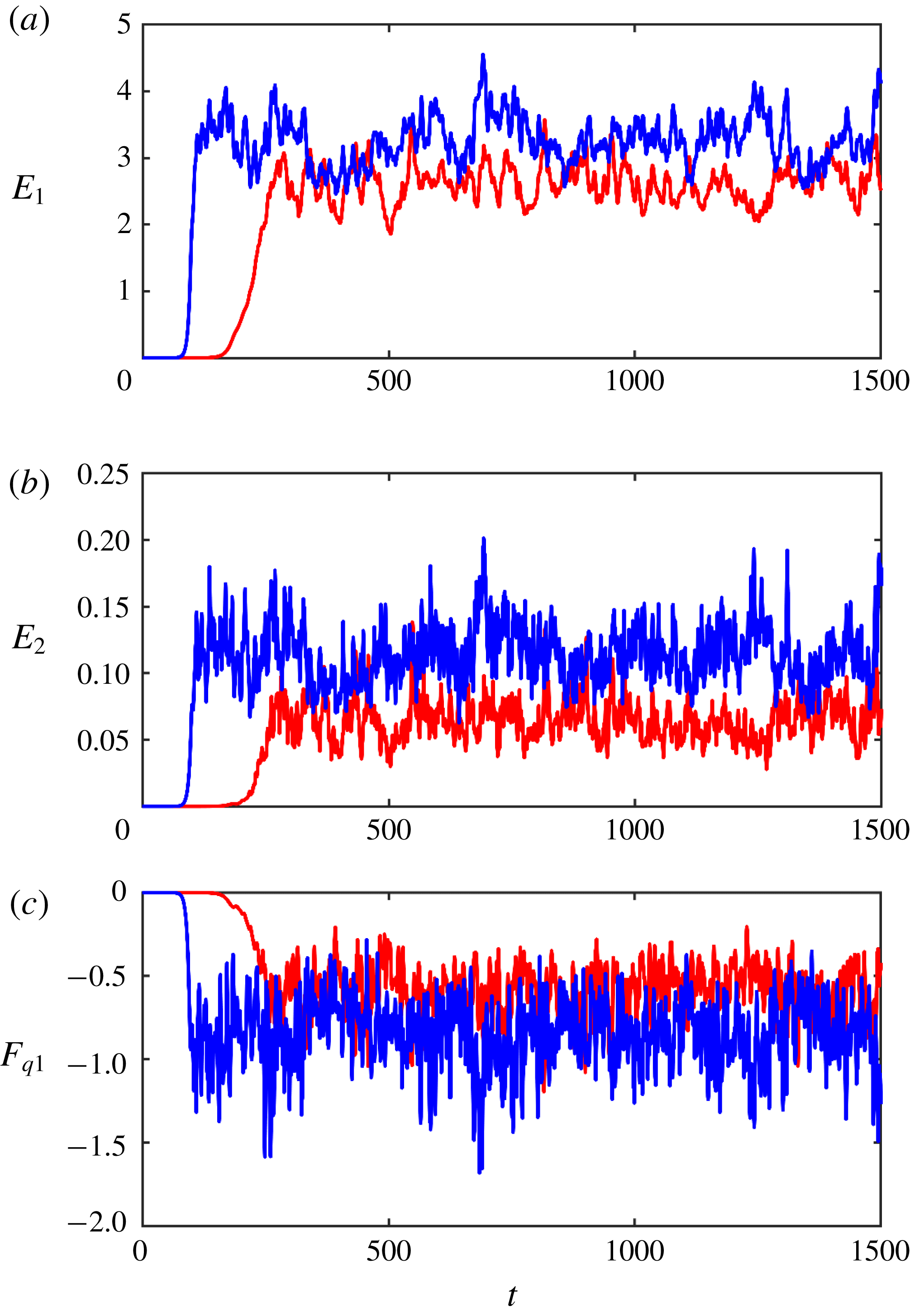
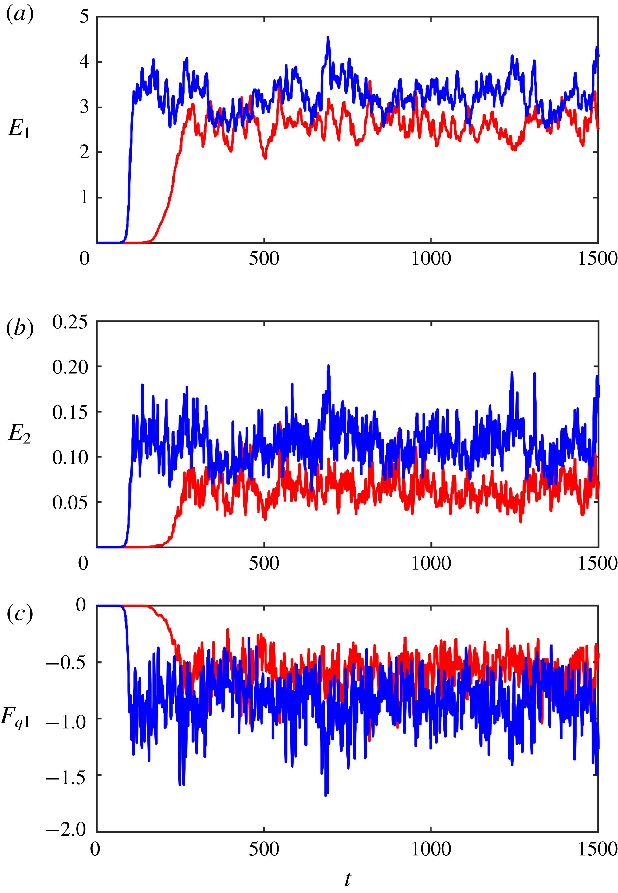
Figure 5 presents the temporal records of
 $(E_{1},E_{2},F_{q1})$
realized in the flat-bottom simulation (blue curves) and in the experiment with variable topography (red curves). All data consistently indicate that small-scale topographic variability adversely affects baroclinic instability. It reduces its growth rate, which almost doubles the period of transition to the quasi-equilibrium regime – from
 $\unicode[STIX]{x0394}t\sim 100$
in the flat-bottom case to
 $\unicode[STIX]{x0394}t\sim 250$
in the variable topography experiment. Even more significant is the notable topographically induced reduction in the equilibrium levels of eddy energy (
 $E_{1}$
,
 $E_{2}$
) and the eddy PV flux
 $|F_{q1}|$
. The following asymptotic multiscale model attempts to explore this effect in detail and parameterize the associated submesoscale dynamics.


3 Multiscale model
To represent mesoscale–submesoscale interactions in a systematic manner, we introduce new spatial variables
 $(x_{S},y_{S})$
that reflect the relatively short wavelength of the topographic pattern. These small-scale variables are related to the original ones through
 $$\begin{eqnarray}(x_{S},y_{S})=\unicode[STIX]{x1D700}^{-1}(x,y),\end{eqnarray}$$
where
 $\unicode[STIX]{x1D700}\ll 1$
is the scale-separation parameter. The spatial derivatives in the governing system (2.9) are replaced accordingly,
 $$\begin{eqnarray}\frac{\unicode[STIX]{x2202}}{\unicode[STIX]{x2202}x}\rightarrow \frac{\unicode[STIX]{x2202}}{\unicode[STIX]{x2202}x}+\unicode[STIX]{x1D700}^{-1}\frac{\unicode[STIX]{x2202}}{\unicode[STIX]{x2202}x_{S}},\quad \frac{\unicode[STIX]{x2202}}{\unicode[STIX]{x2202}y}\rightarrow \frac{\unicode[STIX]{x2202}}{\unicode[STIX]{x2202}y}+\unicode[STIX]{x1D700}^{-1}\frac{\unicode[STIX]{x2202}}{\unicode[STIX]{x2202}y_{S}}.\end{eqnarray}$$
The temporal variability exhibits an even broader range of scales. One of the temporal scales
 $(t_{0})$
reflects the dynamics of mesoscale variability, which is characterized by
 $O(1)$
spatial scales and
 $O(1)$
velocities. Another scale
 $(t_{-1})$
represents relatively rapid changes in fluid properties associated with their advection by mesoscale flows with
 $O(1)$
velocity across the submesoscale topography with spatial scales
 $O(\unicode[STIX]{x1D700})$
. Preliminary simulations (§ 2) indicate that small-scale bathymetric variability exerts a relatively weak but persistent influence on the mesoscale flow pattern. The appropriate scaling for this slow process
 $(t_{2})$
was determined a posteriori. We first tentatively proceeded with the multiscale expansion, discovering in the process that the term representing topographic mesoscale influence is of the order of
 ${\sim}\unicode[STIX]{x1D700}^{2}$
, which implies that the evolution of the mesoscale field due to topography occurs on time scales of
 $O(\unicode[STIX]{x1D700}^{-2})$
. Thus, we introduce three distinct temporal variables,
 $$\begin{eqnarray}t_{-1}=\unicode[STIX]{x1D700}^{-1}t,\quad t_{0}=t,\quad t_{2}=\unicode[STIX]{x1D700}^{2}t,\end{eqnarray}$$
and the time derivatives in the governing system (2.9) are replaced as follows:
 $$\begin{eqnarray}\frac{\unicode[STIX]{x2202}}{\unicode[STIX]{x2202}t}\rightarrow \unicode[STIX]{x1D700}^{-1}\frac{\unicode[STIX]{x2202}}{\unicode[STIX]{x2202}t_{-1}}+\frac{\unicode[STIX]{x2202}}{\unicode[STIX]{x2202}t_{0}}+\unicode[STIX]{x1D700}^{2}\frac{\unicode[STIX]{x2202}}{\unicode[STIX]{x2202}t_{2}}.\end{eqnarray}$$
The lateral viscosity
 $(\unicode[STIX]{x1D708})$
is assumed to be small and therefore it is also rescaled in terms of
 $\unicode[STIX]{x1D700}$
,
 $$\begin{eqnarray}\unicode[STIX]{x1D708}=\unicode[STIX]{x1D700}^{2}\unicode[STIX]{x1D708}_{0},\end{eqnarray}$$
which implies that friction could be significant on scales of submesoscale variability but plays only a secondary role in mesoscale dynamics.
The leading-order mesoscale field in the following model is represented by the fully developed streamfunction fields
 $\overline{\unicode[STIX]{x1D713}}_{i}$
. These fields vary only on spatial scales of baroclinic instability, whereas on temporal scales we admit, in addition to
 $O(1)$
mesoscale variability, the slow drift induced by submesoscale topography,
 $$\begin{eqnarray}\overline{\unicode[STIX]{x1D713}}_{i}=\overline{\unicode[STIX]{x1D713}}_{i}(x,y,t_{0},t_{2}).\end{eqnarray}$$
The corresponding mesoscale PV fields
 $(\overline{q}_{i})$
are defined accordingly. To explore the interaction of the mesoscale field (3.6) with topography
 $\unicode[STIX]{x1D702}_{b}(x_{S},y_{S})$
, the solution for
 $\unicode[STIX]{x1D713}_{i}$
is sought in terms of power series in
 $\unicode[STIX]{x1D700}\ll 1$
,
 $$\begin{eqnarray}\unicode[STIX]{x1D713}_{i}=\overline{\unicode[STIX]{x1D713}}_{i}(x,y,t_{0},t_{2})+\unicode[STIX]{x1D700}\unicode[STIX]{x1D713}_{i}^{(1)}(x,y,x_{S},y_{S},t_{-1},t_{0},t_{2})+\unicode[STIX]{x1D700}^{2}\unicode[STIX]{x1D713}_{i}^{(2)}(x,y,x_{S},y_{S},t_{-1},t_{0},t_{2})+\cdots\end{eqnarray}$$
When (3.2)–(3.5) and (3.7) are substituted into the governing equations (2.9), we discover that the inclusion of topographic variability triggers a streamfunction response at
 $O(\unicode[STIX]{x1D700}^{2})$
and therefore the solution can be constructed for
 $\unicode[STIX]{x1D713}_{i}^{(1)}=0$
. The leading-order balance of governing equations is realized at
 $O(\unicode[STIX]{x1D700}^{-1})$
and it can be reduced to the following form:
 $$\begin{eqnarray}\left.\begin{array}{@{}c@{}}\unicode[STIX]{x1D713}_{i}^{(2)}=0,\quad i=1,\ldots ,(n-1),\\ \displaystyle \frac{\unicode[STIX]{x2202}^{2}\unicode[STIX]{x1D713}_{n}^{(2)}}{\unicode[STIX]{x2202}x_{S}^{2}}+\frac{\unicode[STIX]{x2202}^{2}\unicode[STIX]{x1D713}_{n}^{(2)}}{\unicode[STIX]{x2202}y_{S}^{2}}+\frac{\unicode[STIX]{x1D702}_{b}(x_{S},y_{S})}{r_{n}}=0.\end{array}\right\}\end{eqnarray}$$
Equations (3.8) imply that the leading-order perturbation varies only on small scales and is uniquely determined by topography. The physical interpretation of (3.8) is straightforward – it represents the homogenization of the total potential vorticity in the bottom layer. The latter takes the following non-dimensional form:
 $$\begin{eqnarray}Q_{n}=\unicode[STIX]{x1D6FB}^{2}\unicode[STIX]{x1D713}_{n}+s_{n}(\unicode[STIX]{x1D6F9}_{n-1}-\unicode[STIX]{x1D6F9}_{n})+\unicode[STIX]{x1D6FD}y+\frac{\unicode[STIX]{x1D702}_{b}}{r_{n}}.\end{eqnarray}$$
Since the total potential vorticity is a quasi-conservative quantity, in the absence of strong inhomogeneous forcing it tends to evolve in time toward a uniform distribution. This effect occurs in numerous geophysical configurations (e.g. Rhines & Young Reference Rhines and Young1982) and in the present system it is facilitated by active mesoscale stirring. On scales of
 $(x_{S},y_{S})$
, the variation of the beta term is weak
 $(\unicode[STIX]{x1D6E5}(\unicode[STIX]{x1D6FD}y)\sim \unicode[STIX]{x1D700})$
and so is the variation of the stretching term
 $s_{n}(\unicode[STIX]{x1D6F9}_{n-1}-\unicode[STIX]{x1D6F9}_{n})$
. Thus, the homogenization of PV on small spatial scales demands that
 $\unicode[STIX]{x1D6FB}^{2}\unicode[STIX]{x1D713}_{n}+\unicode[STIX]{x1D702}_{b}/r_{n}=\text{const}$
. For small-scale components of
 $\unicode[STIX]{x1D713}_{n}$
and topography also varying only on small scales, the latter equality can only be satisfied as long as the constant on its right-hand side is zero – which is exactly what (3.8) implies. The resulting PV-homogenization mode
 $\unicode[STIX]{x1D713}_{n}^{(2)}$
will be referred to as the primary submesoscale component.
In order to assess the extent to which the homogenization tendency (3.8) is reflected in numerical simulations (e.g. figure 3), we introduce the following measure of homogenization:
 $$\begin{eqnarray}R_{h}=\frac{\text{rms}(\unicode[STIX]{x1D6FB}^{2}\unicode[STIX]{x1D713}_{sm}+r_{n}^{-1}\unicode[STIX]{x1D702}_{b})}{\text{rms}(r_{n}^{-1}\unicode[STIX]{x1D702}_{b})},\end{eqnarray}$$
where
 $\unicode[STIX]{x1D713}_{sm}$
is the small-scale component of the streamfunction in the bottom layer. In the following calculation,
 $\unicode[STIX]{x1D713}_{sm}$
is constructed as a superposition of Fourier harmonics of
 $\unicode[STIX]{x1D713}_{n}$
with wavelengths not exceeding
 $2d$
. The homogenization variable
 $R_{h}$
was evaluated for a series of simulations in which the wavelength of topography was systematically decreased (figure 6). Figure 6 indicates that the reduction of topographic wavelength – which implies an increase in scale separation
 $(\unicode[STIX]{x1D700}\rightarrow 0)$
– leads to a systematic decrease in
 $R_{h}$
. This homogenization tendency supports the asymptotic result (3.8) and instils confidence in its proposed physical interpretation.
The diagnostic variable
 $R_{h}$
that measures the extent of PV homogenization in the bottom layer is plotted as a function of the wavelength of the topographic pattern. The solid (dashed) curve represents a series of simulations performed with a bottom drag coefficient of
 $\unicode[STIX]{x1D6FE}=1$
(
 $\unicode[STIX]{x1D6FE}=0.1$
).

To proceed with the multiscale model, the harmonic topography (2.12) is expressed in terms of small-scale variables as follows:
 $$\begin{eqnarray}\unicode[STIX]{x1D702}_{b}=\unicode[STIX]{x1D702}_{0}\cos (k_{S}x_{S}+l_{S}y_{S}),\end{eqnarray}$$
where
 $(k_{S},l_{S})=\unicode[STIX]{x1D700}(k,l)$
, which reduces (3.8) to
 $$\begin{eqnarray}\unicode[STIX]{x1D713}_{n}^{(2)}=\frac{1}{r_{n}}\frac{\unicode[STIX]{x1D702}_{0}}{k_{S}^{2}+l_{S}^{2}}\cos (k_{S}x_{S}+l_{S}y_{S}).\end{eqnarray}$$
The next order in our expansion contains the
 $O(1)$
components of the governing equations. At this order, topography still does not trigger a response in any layers except for the bottom one and therefore
 $\unicode[STIX]{x1D713}_{i}^{(3)}=0$
for
 $i=1,\ldots ,(n-1)$
. Collecting all
 $O(1)$
terms, we arrive at
 $$\begin{eqnarray}\left.\begin{array}{@{}c@{}}\displaystyle \frac{\unicode[STIX]{x2202}\overline{q}_{1}}{\unicode[STIX]{x2202}t_{0}}+J(\overline{\unicode[STIX]{x1D713}}_{1},\overline{q}_{1})+\unicode[STIX]{x1D6FD}\frac{\unicode[STIX]{x2202}\overline{\unicode[STIX]{x1D713}}_{1}}{\unicode[STIX]{x2202}x}+s_{1}(1-U_{2})\frac{\unicode[STIX]{x2202}\overline{\unicode[STIX]{x1D713}}_{1}}{\unicode[STIX]{x2202}x}+\frac{\unicode[STIX]{x2202}\overline{q}_{1}}{\unicode[STIX]{x2202}x}=0,\\ \begin{array}{@{}l@{}}\displaystyle \frac{\unicode[STIX]{x2202}\overline{q}_{i}}{\unicode[STIX]{x2202}t_{0}}+J(\overline{\unicode[STIX]{x1D713}}_{i},\overline{q}_{i})+\unicode[STIX]{x1D6FD}\frac{\unicode[STIX]{x2202}\overline{\unicode[STIX]{x1D713}}_{i}}{\unicode[STIX]{x2202}x}+s_{i}(2U_{i}-U_{i-1}-U_{i+1})\frac{\unicode[STIX]{x2202}\overline{\unicode[STIX]{x1D713}}_{i}}{\unicode[STIX]{x2202}x}\\ \displaystyle \quad +\,U_{i}\frac{\unicode[STIX]{x2202}\overline{q}_{i}}{\unicode[STIX]{x2202}x}=0,\quad i=2,\ldots ,(n-1),\end{array}\end{array}\right\}\end{eqnarray}$$
for the upper layers and
 $$\begin{eqnarray}\displaystyle & & \displaystyle \underbrace{\frac{\unicode[STIX]{x2202}\overline{q}_{n}}{\unicode[STIX]{x2202}t_{0}}+J(\overline{\unicode[STIX]{x1D713}}_{n},\overline{q}_{n})+\unicode[STIX]{x1D6FD}\frac{\unicode[STIX]{x2202}\overline{\unicode[STIX]{x1D713}}_{n}}{\unicode[STIX]{x2202}x}-s_{n}U_{n-1}\frac{\unicode[STIX]{x2202}\overline{\unicode[STIX]{x1D713}}_{n}}{\unicode[STIX]{x2202}x}+\unicode[STIX]{x1D6FE}\unicode[STIX]{x1D6FB}^{2}\overline{\unicode[STIX]{x1D713}}_{n}}_{A}\nonumber\\ \displaystyle & & \displaystyle \qquad +\,\underbrace{\frac{\unicode[STIX]{x2202}}{\unicode[STIX]{x2202}t_{-1}}\left(\frac{\unicode[STIX]{x2202}^{2}\unicode[STIX]{x1D713}_{n}^{(3)}}{\unicode[STIX]{x2202}x_{S}^{2}}+\frac{\unicode[STIX]{x2202}^{2}\unicode[STIX]{x1D713}_{n}^{(3)}}{\unicode[STIX]{x2202}y_{S}^{2}}\right)+\frac{\unicode[STIX]{x2202}\overline{\unicode[STIX]{x1D713}}_{n}}{\unicode[STIX]{x2202}x}\frac{\unicode[STIX]{x2202}}{\unicode[STIX]{x2202}y_{S}}\left(\frac{\unicode[STIX]{x2202}^{2}\unicode[STIX]{x1D713}_{n}^{(3)}}{\unicode[STIX]{x2202}x_{S}^{2}}+\frac{\unicode[STIX]{x2202}^{2}\unicode[STIX]{x1D713}_{n}^{(3)}}{\unicode[STIX]{x2202}y_{S}^{2}}\right)-\frac{\unicode[STIX]{x2202}\overline{\unicode[STIX]{x1D713}}_{n}}{\unicode[STIX]{x2202}y}\frac{\unicode[STIX]{x2202}}{\unicode[STIX]{x2202}x_{S}}\left(\frac{\unicode[STIX]{x2202}^{2}\unicode[STIX]{x1D713}_{n}^{(3)}}{\unicode[STIX]{x2202}x_{S}^{2}}+\frac{\unicode[STIX]{x2202}^{2}\unicode[STIX]{x1D713}_{n}^{(3)}}{\unicode[STIX]{x2202}y_{S}^{2}}\right)}_{B}\nonumber\\ \displaystyle & & \displaystyle \quad =\underbrace{\unicode[STIX]{x1D708}_{0}\left(\frac{\unicode[STIX]{x2202}^{4}\unicode[STIX]{x1D713}_{n}^{(2)}}{\unicode[STIX]{x2202}x_{S}^{4}}+2\frac{\unicode[STIX]{x2202}^{4}\unicode[STIX]{x1D713}_{n}^{(2)}}{\unicode[STIX]{x2202}x_{S}^{2}\unicode[STIX]{x2202}y_{S}^{2}}+\frac{\unicode[STIX]{x2202}^{4}\unicode[STIX]{x1D713}_{n}^{(2)}}{\unicode[STIX]{x2202}y_{S}^{4}}\right)+\unicode[STIX]{x1D6FE}\left(\frac{\unicode[STIX]{x2202}^{2}\unicode[STIX]{x1D713}_{n}^{(2)}}{\unicode[STIX]{x2202}x_{S}^{2}}+\frac{\unicode[STIX]{x2202}^{2}\unicode[STIX]{x1D713}_{n}^{(2)}}{\unicode[STIX]{x2202}y_{S}^{2}}\right)+\frac{1}{r_{n}}\left(\frac{\unicode[STIX]{x2202}\unicode[STIX]{x1D713}_{n}^{(2)}}{\unicode[STIX]{x2202}x_{S}}\frac{\unicode[STIX]{x2202}\unicode[STIX]{x1D702}_{b}}{\unicode[STIX]{x2202}y_{S}}-\frac{\unicode[STIX]{x2202}\unicode[STIX]{x1D713}_{n}^{(2)}}{\unicode[STIX]{x2202}y_{S}}\frac{\unicode[STIX]{x2202}\unicode[STIX]{x1D702}_{b}}{\unicode[STIX]{x2202}x_{S}}\right)}_{C}\nonumber\\ \displaystyle & & \displaystyle\end{eqnarray}$$
for the bottom layer. Equation (3.13) essentially describes the evolution of basic mesoscale variability in the upper
 $(n-1)$
layers under the assumption that lateral friction is weak. The bottom layer equation (3.14) is substantially different and contains three distinct groups:
 $A$
,
 $B$
and
 $C$
. Group
 $A$
varies only on large scales and it represents the evolution of the basic mesoscale field in the absence of topographic influences. The terms grouped in
 $C$
vary only on small scales. These terms can be evaluated for any
 $\unicode[STIX]{x1D713}_{n}^{(2)}$
, which, in turn, is given in (3.12). Group
 $B$
depends on the third-order perturbation
 $(\unicode[STIX]{x1D713}_{n}^{(3)})$
and therefore (3.14) implicitly determines
 $\unicode[STIX]{x1D713}_{n}^{(3)}$
. The analysis is simplified by realizing that the average of (3.14) over small-scale variables
 $(x_{S},y_{S})$
requires
 $A=0$
, which reduces (3.14) to
 $$\begin{eqnarray}\displaystyle & & \displaystyle \frac{\unicode[STIX]{x2202}}{\unicode[STIX]{x2202}t_{-1}}\left(\frac{\unicode[STIX]{x2202}^{2}\unicode[STIX]{x1D713}_{n}^{(3)}}{\unicode[STIX]{x2202}x_{S}^{2}}+\frac{\unicode[STIX]{x2202}^{2}\unicode[STIX]{x1D713}_{n}^{(3)}}{\unicode[STIX]{x2202}y_{S}^{2}}\right)+\frac{\unicode[STIX]{x2202}\overline{\unicode[STIX]{x1D713}}_{n}}{\unicode[STIX]{x2202}x}\frac{\unicode[STIX]{x2202}}{\unicode[STIX]{x2202}y_{S}}\left(\frac{\unicode[STIX]{x2202}^{2}\unicode[STIX]{x1D713}_{n}^{(3)}}{\unicode[STIX]{x2202}x_{S}^{2}}+\frac{\unicode[STIX]{x2202}^{2}\unicode[STIX]{x1D713}_{n}^{(3)}}{\unicode[STIX]{x2202}y_{S}^{2}}\right)\nonumber\\ \displaystyle & & \displaystyle \quad -\,\frac{\unicode[STIX]{x2202}\overline{\unicode[STIX]{x1D713}}_{n}}{\unicode[STIX]{x2202}y}\frac{\unicode[STIX]{x2202}}{\unicode[STIX]{x2202}x_{S}}\left(\frac{\unicode[STIX]{x2202}^{2}\unicode[STIX]{x1D713}_{n}^{(3)}}{\unicode[STIX]{x2202}x_{S}^{2}}+\frac{\unicode[STIX]{x2202}^{2}\unicode[STIX]{x1D713}_{n}^{(3)}}{\unicode[STIX]{x2202}y_{S}^{2}}\right)=C.\end{eqnarray}$$
To determine
 $\unicode[STIX]{x1D713}_{n}^{(3)}$
, we seek the solution in the following form:
 $$\begin{eqnarray}\unicode[STIX]{x1D713}_{n}^{(3)}=\unicode[STIX]{x1D711}_{C}(x,y,t_{-1},t_{0},t_{2})\cos (k_{S}x_{S}+l_{S}y_{S})+\unicode[STIX]{x1D711}_{S}(x,y,t_{-1},t_{0},t_{2})\sin (k_{S}x_{S}+l_{S}y_{S}).\end{eqnarray}$$
When (3.12) and (3.16) are substituted into (3.15), we arrive at
 $$\begin{eqnarray}\left.\begin{array}{@{}c@{}}\displaystyle \frac{\unicode[STIX]{x2202}\unicode[STIX]{x1D711}_{C}}{\unicode[STIX]{x2202}t_{-1}}=-\frac{\unicode[STIX]{x1D702}_{0}}{r_{n}}\frac{(k_{S}^{2}+l_{S}^{2})\unicode[STIX]{x1D708}_{0}+\unicode[STIX]{x1D6FE}}{k_{S}^{2}+l_{S}^{2}}+\unicode[STIX]{x1D711}_{S}\left(\frac{\unicode[STIX]{x2202}\overline{\unicode[STIX]{x1D713}}_{n}}{\unicode[STIX]{x2202}y}k_{S}-\frac{\unicode[STIX]{x2202}\overline{\unicode[STIX]{x1D713}}_{n}}{\unicode[STIX]{x2202}x}l_{S}\right),\\ \displaystyle \frac{\unicode[STIX]{x2202}\unicode[STIX]{x1D711}_{S}}{\unicode[STIX]{x2202}t_{-1}}=-\unicode[STIX]{x1D711}_{C}\left(\frac{\unicode[STIX]{x2202}\overline{\unicode[STIX]{x1D713}}_{n}}{\unicode[STIX]{x2202}y}k_{S}-\frac{\unicode[STIX]{x2202}\overline{\unicode[STIX]{x1D713}}_{n}}{\unicode[STIX]{x2202}x}l_{S}\right).\end{array}\right\}\end{eqnarray}$$
Equations (3.15)–(3.17) are physically interpreted as the generation of the secondary submesoscale pattern
 $(\unicode[STIX]{x1D713}_{n}^{(3)})$
in response to the system forcing by the primary submesoscale pattern
 $(\unicode[STIX]{x1D713}_{n}^{(2)})$
.
The expansion is extended in a similar manner to the
 $O(\unicode[STIX]{x1D700})$
balance of the governing equations, which yields
 $$\begin{eqnarray}\left.\begin{array}{@{}c@{}}\displaystyle \begin{array}{@{}rcl@{}}\displaystyle \frac{\unicode[STIX]{x2202}\unicode[STIX]{x1D711}_{C}}{\unicode[STIX]{x2202}t_{0}}\; & =\; & \displaystyle J_{xy}(\unicode[STIX]{x1D711}_{C},\overline{\unicode[STIX]{x1D713}}_{n})+2\unicode[STIX]{x1D711}_{C}\frac{\displaystyle (l_{S}^{2}-k_{S}^{2})\frac{\unicode[STIX]{x2202}^{2}\overline{\unicode[STIX]{x1D713}}_{n}}{\unicode[STIX]{x2202}x\unicode[STIX]{x2202}y}+k_{S}l_{S}\left(\frac{\unicode[STIX]{x2202}^{2}\overline{\unicode[STIX]{x1D713}}_{n}}{\unicode[STIX]{x2202}x^{2}}-\frac{\unicode[STIX]{x2202}^{2}\overline{\unicode[STIX]{x1D713}}_{n}}{\unicode[STIX]{x2202}y^{2}}\right)}{k_{S}^{2}+l_{S}^{2}}\\ \; & \; & \displaystyle -\,\unicode[STIX]{x1D711}_{C}(k_{S}^{2}\unicode[STIX]{x1D708}_{0}+l_{S}^{2}\unicode[STIX]{x1D708}_{0}+\unicode[STIX]{x1D6FE}),\end{array}\\ \displaystyle \begin{array}{@{}rcl@{}}\displaystyle \frac{\unicode[STIX]{x2202}\unicode[STIX]{x1D711}_{S}}{\unicode[STIX]{x2202}t_{0}}\; & =\; & \displaystyle J_{xy}(\unicode[STIX]{x1D711}_{S},\overline{\unicode[STIX]{x1D713}}_{n})+2\unicode[STIX]{x1D711}_{S}\frac{\displaystyle (l_{S}^{2}-k_{S}^{2})\frac{\unicode[STIX]{x2202}^{2}\overline{\unicode[STIX]{x1D713}}_{n}}{\unicode[STIX]{x2202}x\unicode[STIX]{x2202}y}+k_{S}l_{S}\left(\frac{\unicode[STIX]{x2202}^{2}\overline{\unicode[STIX]{x1D713}}_{n}}{\unicode[STIX]{x2202}x^{2}}-\frac{\unicode[STIX]{x2202}^{2}\overline{\unicode[STIX]{x1D713}}_{n}}{\unicode[STIX]{x2202}y^{2}}\right)}{k_{S}^{2}+l_{S}^{2}}\\ \; & \; & \displaystyle -\,\unicode[STIX]{x1D711}_{S}(k_{S}^{2}\unicode[STIX]{x1D708}_{0}+l_{S}^{2}\unicode[STIX]{x1D708}_{0}+\unicode[STIX]{x1D6FE})\\ \; & \; & +\,\displaystyle \frac{\unicode[STIX]{x1D702}_{0}}{r_{n}}\frac{\displaystyle \frac{\unicode[STIX]{x2202}}{\unicode[STIX]{x2202}x}\unicode[STIX]{x1D6FB}^{2}\overline{\unicode[STIX]{x1D713}}_{n}l_{S}-\frac{\unicode[STIX]{x2202}}{\unicode[STIX]{x2202}y}\unicode[STIX]{x1D6FB}^{2}\overline{\unicode[STIX]{x1D713}}_{n}k_{S}+s_{n}\frac{\unicode[STIX]{x2202}\overline{\unicode[STIX]{x1D713}}_{n-1}}{\unicode[STIX]{x2202}x}l_{S}-k_{S}\left(\frac{\unicode[STIX]{x2202}\overline{\unicode[STIX]{x1D713}}_{n-1}}{\unicode[STIX]{x2202}y}s_{n}-s_{n}U_{n-1}+\unicode[STIX]{x1D6FD}\right)}{(k_{S}^{2}+l_{S}^{2})^{2}}.\end{array}\end{array}\right\}\end{eqnarray}$$
The notation
 $J_{xy}$
for the Jacobian is used here to emphasize that the derivatives are taken in large-scale variables
 $(x,y)$
. The terms representing the influence of topography on mesoscale fields are obtained as a solvability condition at the next order, by averaging the
 $O(\unicode[STIX]{x1D700}^{2})$
balances of the governing equations in
 $(x_{S},y_{S})$
. For the upper layers, we obtain
 $$\begin{eqnarray}\frac{\unicode[STIX]{x2202}}{\unicode[STIX]{x2202}t_{2}}\overline{q}_{i}-\unicode[STIX]{x1D708}_{0}\left(\frac{\unicode[STIX]{x2202}^{4}\overline{\unicode[STIX]{x1D713}}_{i}}{\unicode[STIX]{x2202}x^{4}}+2\frac{\unicode[STIX]{x2202}^{4}\overline{\unicode[STIX]{x1D713}}_{i}}{\unicode[STIX]{x2202}x^{2}\unicode[STIX]{x2202}y^{2}}+\frac{\unicode[STIX]{x2202}^{4}\overline{\unicode[STIX]{x1D713}}_{i}}{\unicode[STIX]{x2202}y^{4}}\right)=0,\quad i=1,\ldots ,(n-1).\end{eqnarray}$$
The corresponding mesoscale balance for the lower layer amounts to
 $$\begin{eqnarray}\frac{\unicode[STIX]{x2202}}{\unicode[STIX]{x2202}t_{2}}\overline{q}_{n}+D-\unicode[STIX]{x1D708}_{0}\left(\frac{\unicode[STIX]{x2202}^{4}\overline{\unicode[STIX]{x1D713}}_{n}}{\unicode[STIX]{x2202}x^{4}}+2\frac{\unicode[STIX]{x2202}^{4}\overline{\unicode[STIX]{x1D713}}_{n}}{\unicode[STIX]{x2202}x^{2}\unicode[STIX]{x2202}y^{2}}+\frac{\unicode[STIX]{x2202}^{4}\overline{\unicode[STIX]{x1D713}}_{n}}{\unicode[STIX]{x2202}y^{4}}\right)=0,\end{eqnarray}$$
where
 $$\begin{eqnarray}D=\frac{\unicode[STIX]{x1D702}_{0}}{2r_{n}}\left(\frac{\unicode[STIX]{x2202}\unicode[STIX]{x1D711}_{S}}{\unicode[STIX]{x2202}y}k_{S}-\frac{\unicode[STIX]{x2202}\unicode[STIX]{x1D711}_{S}}{\unicode[STIX]{x2202}x}l_{S}\right).\end{eqnarray}$$
The mesoscale term
 $D$
is a result of the interaction between the primary submesoscale component (the PV-homogenization mode
 $\unicode[STIX]{x1D713}_{n}^{(2)}$
) and the secondary submesoscale response
 $(\unicode[STIX]{x1D713}_{n}^{(3)})$
. Since the small-scale patterns of
 $\unicode[STIX]{x1D713}_{n}^{(2)}$
and
 $\unicode[STIX]{x1D713}_{n}^{(3)}$
are not entirely orthogonal, their nonlinear interaction produces a finite mesoscale response. This effect accounts for the modification of baroclinic instability properties by submesoscale topography.
At this point, the multiscale analysis is complete and we can return to the original variables by reverting the transformation (3.4),
 $$\begin{eqnarray}\left.\begin{array}{@{}c@{}}\displaystyle \frac{\unicode[STIX]{x2202}\overline{q}_{1}}{\unicode[STIX]{x2202}t}+J(\overline{\unicode[STIX]{x1D713}}_{1},\overline{q}_{1})+\unicode[STIX]{x1D6FD}\frac{\unicode[STIX]{x2202}\overline{\unicode[STIX]{x1D713}}_{1}}{\unicode[STIX]{x2202}x}+s_{1}(1-U_{2})\frac{\unicode[STIX]{x2202}\overline{\unicode[STIX]{x1D713}}_{1}}{\unicode[STIX]{x2202}x}+\frac{\unicode[STIX]{x2202}\overline{q}_{1}}{\unicode[STIX]{x2202}x}=\unicode[STIX]{x1D708}\unicode[STIX]{x1D6FB}^{4}\overline{\unicode[STIX]{x1D713}}_{1},\\ \displaystyle \begin{array}{@{}l@{}}\displaystyle \frac{\unicode[STIX]{x2202}\overline{q}_{i}}{\unicode[STIX]{x2202}t}+J(\overline{\unicode[STIX]{x1D713}}_{i},\overline{q}_{i})+\unicode[STIX]{x1D6FD}\frac{\unicode[STIX]{x2202}\overline{\unicode[STIX]{x1D713}}_{i}}{\unicode[STIX]{x2202}x}+s_{i}(2U_{i}-U_{i-1}-U_{i+1})\frac{\unicode[STIX]{x2202}\overline{\unicode[STIX]{x1D713}}_{i}}{\unicode[STIX]{x2202}x}\\ \displaystyle \quad +\,U_{i}\frac{\unicode[STIX]{x2202}\overline{q}_{i}}{\unicode[STIX]{x2202}x}=0,\quad i=2,\ldots ,(n-1),\end{array}\\ \displaystyle \frac{\unicode[STIX]{x2202}\overline{q}_{n}}{\unicode[STIX]{x2202}t}+J(\overline{\unicode[STIX]{x1D713}}_{n},\overline{q}_{n})+\unicode[STIX]{x1D6FD}\frac{\unicode[STIX]{x2202}\overline{\unicode[STIX]{x1D713}}_{n}}{\unicode[STIX]{x2202}x}-s_{n}U_{n-1}\frac{\unicode[STIX]{x2202}\overline{\unicode[STIX]{x1D713}}_{n}}{\unicode[STIX]{x2202}x}+\unicode[STIX]{x1D6FE}\unicode[STIX]{x1D6FB}^{2}\overline{\unicode[STIX]{x1D713}}_{n}+\overline{D}=\unicode[STIX]{x1D708}\unicode[STIX]{x1D6FB}^{4}\overline{\unicode[STIX]{x1D713}}_{2},\end{array}\right\}\end{eqnarray}$$
where
 $$\begin{eqnarray}\overline{D}=\unicode[STIX]{x1D700}^{2}D.\end{eqnarray}$$
The comparison of the mesoscale system (3.22) with governing equations (2.9) is revealing. It shows that the submesoscale topographic forcing term
 $J(\unicode[STIX]{x1D713}_{n},\unicode[STIX]{x1D702}_{b})/r_{n}$
in (2.9) is now replaced by the mesoscale term
 $\overline{D}$
. The final step in formulating the closed mesoscale system is the calculation of
 $(\unicode[STIX]{x1D711}_{C},\unicode[STIX]{x1D711}_{S})$
, which is accomplished by evaluating the two leading tendency terms,
 $$\begin{eqnarray}\frac{\unicode[STIX]{x2202}}{\unicode[STIX]{x2202}t}\left(\begin{array}{@{}c@{}}\unicode[STIX]{x1D711}_{C}\\ \unicode[STIX]{x1D711}_{S}\end{array}\right)=\unicode[STIX]{x1D700}^{-1}\frac{\unicode[STIX]{x2202}}{\unicode[STIX]{x2202}t_{-1}}\left(\begin{array}{@{}c@{}}\unicode[STIX]{x1D711}_{C}\\ \unicode[STIX]{x1D711}_{S}\end{array}\right)+\frac{\unicode[STIX]{x2202}}{\unicode[STIX]{x2202}t_{0}}\left(\begin{array}{@{}c@{}}\unicode[STIX]{x1D711}_{C}\\ \unicode[STIX]{x1D711}_{S}\end{array}\right)+O(\unicode[STIX]{x1D700}^{2}).\end{eqnarray}$$
The inclusion of two terms in (3.24), instead of retaining just the single leading-order component, makes it possible to construct the parametric model of the submesoscale topography with a relative error of only
 $O(\unicode[STIX]{x1D700}^{2})$
. Such a model can be expected to retain its predictive capabilities even in cases when the scale separation between the interacting flow components is limited – the situation which is probably realized in most ocean regions.
The substitution of (3.17) and (3.18) in (3.24) yields
 $$\begin{eqnarray}\left.\begin{array}{@{}c@{}}\displaystyle \begin{array}{@{}rcl@{}}\displaystyle \frac{\unicode[STIX]{x2202}\overline{\unicode[STIX]{x1D711}}_{C}}{\unicode[STIX]{x2202}t}\; & =\; & \displaystyle -\frac{\unicode[STIX]{x1D702}_{0}}{r_{n}}\frac{(k^{2}+l^{2})\unicode[STIX]{x1D708}+\unicode[STIX]{x1D6FE}}{k^{2}+l^{2}}+\overline{\unicode[STIX]{x1D711}}_{S}\left(\frac{\unicode[STIX]{x2202}\overline{\unicode[STIX]{x1D713}}_{n}}{\unicode[STIX]{x2202}y}k-\frac{\unicode[STIX]{x2202}\overline{\unicode[STIX]{x1D713}}_{n}}{\unicode[STIX]{x2202}x}l\right)\\ \; & \; & \displaystyle +\,J_{xy}(\overline{\unicode[STIX]{x1D711}}_{C},\overline{\unicode[STIX]{x1D713}}_{n})-\overline{\unicode[STIX]{x1D711}}_{C}(k^{2}\unicode[STIX]{x1D708}+l^{2}\unicode[STIX]{x1D708}+\unicode[STIX]{x1D6FE})\\ \; & \; & +\,\displaystyle 2\overline{\unicode[STIX]{x1D711}}_{C}\frac{\displaystyle (l^{2}-k^{2})\frac{\unicode[STIX]{x2202}^{2}\overline{\unicode[STIX]{x1D713}}_{n}}{\unicode[STIX]{x2202}x\unicode[STIX]{x2202}y}+kl\left(\frac{\unicode[STIX]{x2202}^{2}\overline{\unicode[STIX]{x1D713}}_{n}}{\unicode[STIX]{x2202}x^{2}}-\frac{\unicode[STIX]{x2202}^{2}\overline{\unicode[STIX]{x1D713}}_{n}}{\unicode[STIX]{x2202}y^{2}}\right)}{k^{2}+l^{2}},\end{array}\\ \displaystyle \begin{array}{@{}rcl@{}}\displaystyle \frac{\unicode[STIX]{x2202}\overline{\unicode[STIX]{x1D711}}_{S}}{\unicode[STIX]{x2202}t}\; & =\; & \displaystyle -\overline{\unicode[STIX]{x1D711}}_{C}\left(\frac{\unicode[STIX]{x2202}\overline{\unicode[STIX]{x1D713}}_{n}}{\unicode[STIX]{x2202}y}k-\frac{\unicode[STIX]{x2202}\overline{\unicode[STIX]{x1D713}}_{n}}{\unicode[STIX]{x2202}x}l\right)+J_{xy}(\overline{\unicode[STIX]{x1D711}}_{S},\overline{\unicode[STIX]{x1D713}}_{n})\\ \; & \; & \displaystyle +\,2\overline{\unicode[STIX]{x1D711}}_{S}\frac{\displaystyle (l^{2}-k^{2})\frac{\unicode[STIX]{x2202}^{2}\overline{\unicode[STIX]{x1D713}}_{n}}{\unicode[STIX]{x2202}x\unicode[STIX]{x2202}y}+kl\left(\frac{\unicode[STIX]{x2202}^{2}\overline{\unicode[STIX]{x1D713}}_{n}}{\unicode[STIX]{x2202}x^{2}}-\frac{\unicode[STIX]{x2202}^{2}\overline{\unicode[STIX]{x1D713}}_{n}}{\unicode[STIX]{x2202}y^{2}}\right)}{k^{2}+l^{2}}\\ \; & \; & +\,\displaystyle \frac{\unicode[STIX]{x1D702}_{0}}{r_{n}}\frac{\displaystyle \frac{\unicode[STIX]{x2202}}{\unicode[STIX]{x2202}x}\unicode[STIX]{x1D6FB}^{2}\overline{\unicode[STIX]{x1D713}}_{n}l-\frac{\unicode[STIX]{x2202}}{\unicode[STIX]{x2202}y}\unicode[STIX]{x1D6FB}^{2}\overline{\unicode[STIX]{x1D713}}_{n}k+s_{n}\frac{\unicode[STIX]{x2202}\overline{\unicode[STIX]{x1D713}}_{n-1}}{\unicode[STIX]{x2202}x}l-k\left(\frac{\unicode[STIX]{x2202}\overline{\unicode[STIX]{x1D713}}_{n-1}}{\unicode[STIX]{x2202}y}s_{n}-s_{n}U_{n-1}+\unicode[STIX]{x1D6FD}\right)}{(k^{2}+l^{2})^{2}}\\ \; & \; & \displaystyle -\,\overline{\unicode[STIX]{x1D711}}_{S}(k^{2}\unicode[STIX]{x1D708}+l^{2}\unicode[STIX]{x1D708}+\unicode[STIX]{x1D6FE}),\end{array}\end{array}\right\}\end{eqnarray}$$
where
 $(\overline{\unicode[STIX]{x1D711}}_{C},\overline{\unicode[STIX]{x1D711}}_{S})=\unicode[STIX]{x1D700}^{3}(\unicode[STIX]{x1D711}_{C},\unicode[STIX]{x1D711}_{S})$
. The topographic forcing term
 $\overline{D}$
in (3.22) is then expressed in terms of
 $\overline{\unicode[STIX]{x1D711}}_{S}$
using (3.21)
 $$\begin{eqnarray}\overline{D}=\frac{\unicode[STIX]{x1D702}_{0}}{2r_{n}}\left(\frac{\unicode[STIX]{x2202}\overline{\unicode[STIX]{x1D711}}_{S}}{\unicode[STIX]{x2202}y}k-\frac{\unicode[STIX]{x2202}\overline{\unicode[STIX]{x1D711}}_{S}}{\unicode[STIX]{x2202}x}l\right).\end{eqnarray}$$
Equations (3.22), (3.25) and (3.26) represent a closed system written entirely in terms of mesoscale variables. Therefore, this model can be viewed as a rigorous parameterization of topographically induced submesoscale variability. While the new set contains two additional prognostic equations (3.25), this disadvantage is outweighed by its ability to represent the submesoscale dynamics without explicitly resolving it.
4 Results
The objective of this section is twofold: (i) the systematic exploration of the influence of submesoscale topography on the properties baroclinic instability for a wide range of governing parameters and (ii) the assessment of the performance of the multiscale model (§ 3), which is achieved by comparing the parameterized and submesoscale-resolving simulations. The investigation starts with a detailed analysis of the two-layer model (§ 4.1) and is followed by an abbreviated discussion of the corresponding multilayer
 $(n>2)$
solutions in § 4.2.
4.1 Two-layer model
The analysis is based on the equilibrium values of kinetic energy and the meridional PV flux
 $(E_{1},E_{2},F_{q1})$
as the key diagnostic variables. These equilibrium values are computed by integrating the model equations, both original and parametric, over extended periods of time (for 1500 non-dimensional units at the minimum). The time records of
 $(E_{1},E_{2},F_{q1})$
are then averaged over the second half of each simulation, thereby excluding from averaging the period of system transition to the quasi-equilibrium regime (e.g. figure 4).
Of particular interest is the sensitivity of the equilibrium energy and PV flux – denoted as
 $(\overline{E}_{1},\overline{E}_{2},\overline{F}_{q1})$
– to the amplitude of topographic variability (
 $\unicode[STIX]{x1D702}_{0}$
), its orientation
 $(\unicode[STIX]{x1D703})$
and the wavelength
 $d=(2\unicode[STIX]{x03C0})/\sqrt{k^{2}+l^{2}}$
. The orientation variable is implicitly defined by
 $$\begin{eqnarray}\cos (\unicode[STIX]{x1D703})=\frac{k}{\sqrt{k^{2}+l^{2}}},\quad \sin (\unicode[STIX]{x1D703})=\frac{l}{\sqrt{k^{2}+l^{2}}},\end{eqnarray}$$
and therefore zonal topography corresponds to
 $\unicode[STIX]{x1D703}=\unicode[STIX]{x03C0}/2$
(e.g. figure 3), while
 $\unicode[STIX]{x1D703}=0$
represents the meridional orientation. Without loss of generality, we explore the orientation effects within the interval
 $0\leqslant \unicode[STIX]{x1D703}<\unicode[STIX]{x03C0}$
. Since the parametric system (3.22), (3.25) and (3.26) does not require the resolution of submesoscale features, its integrations are performed on the mesh with
 $N_{x}\times N_{y}=256\times 256$
grid points, which is much coarser than that one used in submesoscale-resolving calculations
 $(N_{x}\times N_{y}=1024\times 1024)$
. Other parameters, which are listed in (2.11), are kept the same as in the baseline experiments (§ 3).
Figure 7 presents a series of simulations with various amplitudes of topography for
 $\unicode[STIX]{x1D703}=\unicode[STIX]{x03C0}/2$
and
 $d=0.15$
. The predictions of parametric and topography-resolving models are mutually consistent. In both models, the increase in bottom variability results in the dramatic reduction in the intensity of both eddy kinetic energy and PV transport. Even a rather modest amplitude of
 $\unicode[STIX]{x1D702}_{0}=9$
, which corresponds to the dimensional topographic variation of only 170 m in the 4 km deep ocean, produces a threefold reduction in the upper layer energy (
 $\overline{E}_{1}$
) and a fivefold reduction in the PV flux
 $(|\overline{F}_{q1}|)$
. This result is particularly striking in view of the indirect manner in which topography influences the upper layer dynamics. Topography enters into parametric system (3.22) only through the forcing term in the lower layer equation – the upper layer equation does not explicitly reflect the non-uniformity of depth. Submesoscale-resolving simulations also reflect no visible presence of submesoscale features in the upper layer (e.g. figure 3). Yet, the impact of submesoscale topography on the upper layer eddies is adverse and profound. It is possible that this result reflects the role of the barotropic mode, which is directly influenced by topography, in the equilibration of baroclinic instability.
The mean values of kinetic energy in the upper layer (a), kinetic energy in the lower layer (b) and the upper layer PV flux (c) as functions of the amplitude of topographic variation. The blue (red) curves represent topography-resolving (parametric) simulations.

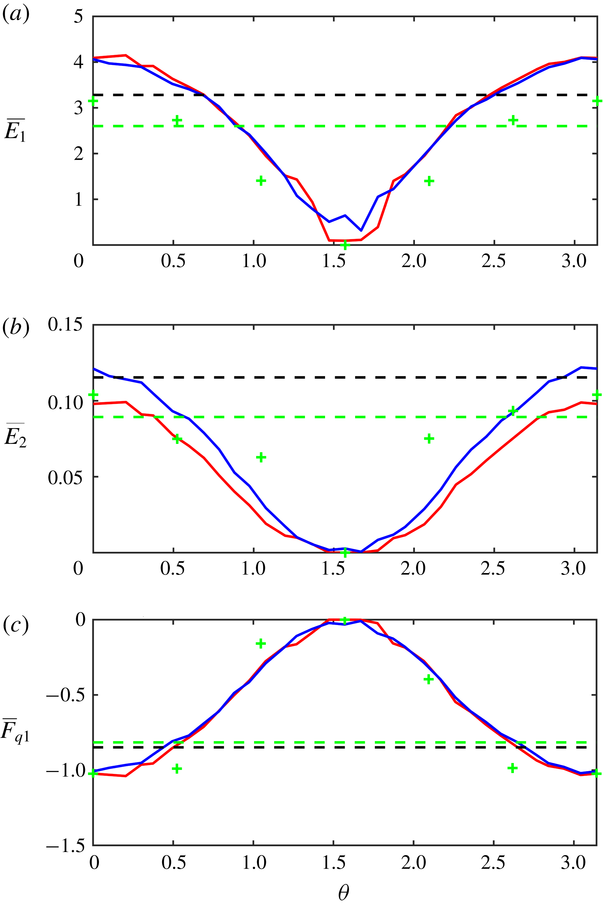
The sensitivity of baroclinic instability to the orientation of bottom topography for
 $\unicode[STIX]{x1D702}_{0}=4.5$
and
 $d=0.15$
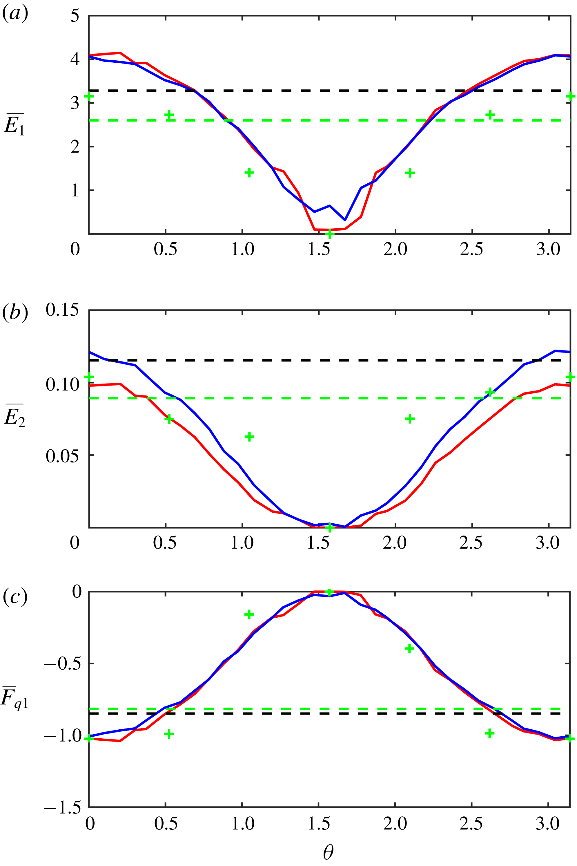
is illustrated in figure 8. It indicates that the zonally oriented topography
 $(\unicode[STIX]{x1D703}=\unicode[STIX]{x03C0}/2)$
is particularly effective in suppressing mesoscale variability. This result can be physically rationalized by recalling that the most rapidly amplifying modes of baroclinic instability take the form of meridional currents (e.g. Phillips Reference Phillips1951; Pedlosky Reference Pedlosky1975). Therefore, a zonally orientated topography presents an apparent obstacle to their growth, adversely affecting baroclinic instability even in the fully nonlinear regime. The meridional topography, on the other hand, does not directly interact with amplifying meridional modes and therefore its impact on baroclinic instability is less pronounced. The meridional topography actually tends to slightly intensify the mesoscale eddy activity in the upper layer relative to that in the flat-bottom case, which is indicated in figure 6 by the horizontal dashed lines. The latter effect can be attributed to the topographic suppression of secondary instabilities of primary meridional modes. It has been suggested that the equilibrium state of baroclinic instability is controlled by the interaction between primary modes and their secondary instabilities (e.g. Pedlosky Reference Pedlosky1975; Radko, Peixoto de Carvalho & Flanagan Reference Radko, Peixoto de Carvalho and Flanagan2014). Thus, the suppression of secondary instabilities by meridional topography weakens one of the potentially significant equilibration mechanisms, thereby allowing baroclinic instability to be more intense than in the flat-bottom case.
The mean values of kinetic energy in the upper layer (a), kinetic energy in the lower layer (b) and the upper layer PV flux (c) as functions of the orientation of topography. The blue (red) curves represent topography-resolving (parametric) simulations. The wavelength of topographic patterns is
 $d=0.15$
. The horizontal dashed lines represent the corresponding flat-bottom simulation.

The impressive agreement between parametric and topography-resolving simulations in figures 7 and 8 underscores the power and utility of multiscale modelling on which the proposed parameterization is based. In this regard, it should be emphasized that the multiscale method formally assumes that the interacting components operate on asymptotically dissimilar scales (
 $\unicode[STIX]{x1D700}\ll 1$
). The successful performance of the parametric model in the regime where scale separation is rather limited (
 $d=0.15$
) suggests that this assumption may not be critical. To further explore this issue, we have reproduced the foregoing calculation (figure 8) with an even larger wavelength of
 $d=0.5$
– the regime in which scale separation is virtually non-existent. The dimensional scale of topographic variability in this case is
 $d^{\ast }=30~\text{km}$
, which places it in the mesoscale, rather than submesoscale, range. Nevertheless, even under these unfavourable conditions, the model performs surprisingly well, particularly in its description of the upper layer properties –
 $\overline{E}_{1}(\unicode[STIX]{x1D703})$
in figure 9(a) and
 $\overline{F}_{q1}(\unicode[STIX]{x1D703})$
in figure 9(c). Some systematic differences between parametric and topography-resolving models can be detected in their lower layer energy patterns (figure 9
b), but these differences are relatively small
 $({\sim}20\,\%)$
and the qualitative similarity of two models is still apparent.

Typical patterns of PV realized in the quasi-equilibrium phase (
 $t=2000$
) of the four-layer simulation.

In addition to these quasi-geostrophic results, figure 9 also presents the corresponding topography-resolving simulations performed using a more general shallow-water model (appendix B). Their general consistency implies that non-quasi-geostrophic effects are not critical for the system considered in the present investigation.
4.2 Multi-layer solutions
While two-layer solutions are suggestive and dynamically transparent, their quantitative applicability can be readily questioned. Of particular concern is the possibility that crude vertical discretization of the foregoing model could lead to an exaggeration of topographic effects. By design, the horizontal velocity components are vertically uniform over the entire abyssal layer
 $-H<z<-H_{1}$
and therefore much of the model ocean is directly influenced by topographic features. Would such sensitivity of baroclinic instability to the bottom topography persist in models with a more sophisticated and realistic representation of stratification? To alleviate such concerns, we present a series of simulations – parametric and topography resolving – in which the number of layers
 $(n)$
is systematically increased. We consider density layers of equal thickness
 $(r_{i}=1/n)$
and a velocity pattern characterized by the linear variation with depth,
 $$\begin{eqnarray}U_{i}=\frac{n-i}{n-1},\quad i=1,\ldots ,n.\end{eqnarray}$$
The topographic variability is represented by (2.12) with
 $\unicode[STIX]{x1D702}_{0}=2$
and zonal orientation
 $(\unicode[STIX]{x1D703}=\unicode[STIX]{x03C0}/2)$
. To ensure that the layer thickness greatly exceeds the variation in topography, which is one of the basic assumptions of the quasi-geostrophic approximation, the number of layers is kept at
 $n=8$
or less.
Typical patterns of baroclinic instability realized in the multi-layer
 $(n>2)$
model are qualitatively similar to their two-layer counterparts. Figure 10 presents PV fields
 $(q_{i})$
in the four-layer system that are realized in the quasi-equilibrium evolutionary stage
 $(t=2000)$
. While the bottom layer exhibits visible modulation on the scales set by topography (figure 10
d), such variability is notably absent in all other layers (figure 10
a–c). However, despite the lack of readily identifiable submesoscale features in most of the model ocean, submesoscale topography dramatically alters the intensity and transport characteristics of baroclinic instability throughout the entire domain. This conclusion is quantified by figure 11, where we plot the mean values of kinetic energy and meridional PV flux in the sub-surface
 $(i=1)$
and bottom
 $(i=n)$
layers for each of seven simulations
 $(n=2,\ldots ,8)$
performed with the original quasi-geostrophic (blue dots) and parametric (red dots) models. For reference, we also present the corresponding flat-bottom experiments (black dots).
Multi-layer solutions. The mean values of kinetic energy in the top (
 $i=1$
) and bottom (
 $i=n$
) layers are plotted as a function of the total number of layers (
 $n$
) in (a,b). The corresponding mean values of the PV flux are shown in (c,d). The flat-bottom simulations are represented by black dots, whereas the variable topography experiments performed with the original quasi-geostrophic and parametric models are indicated by blue and red dots respectively.
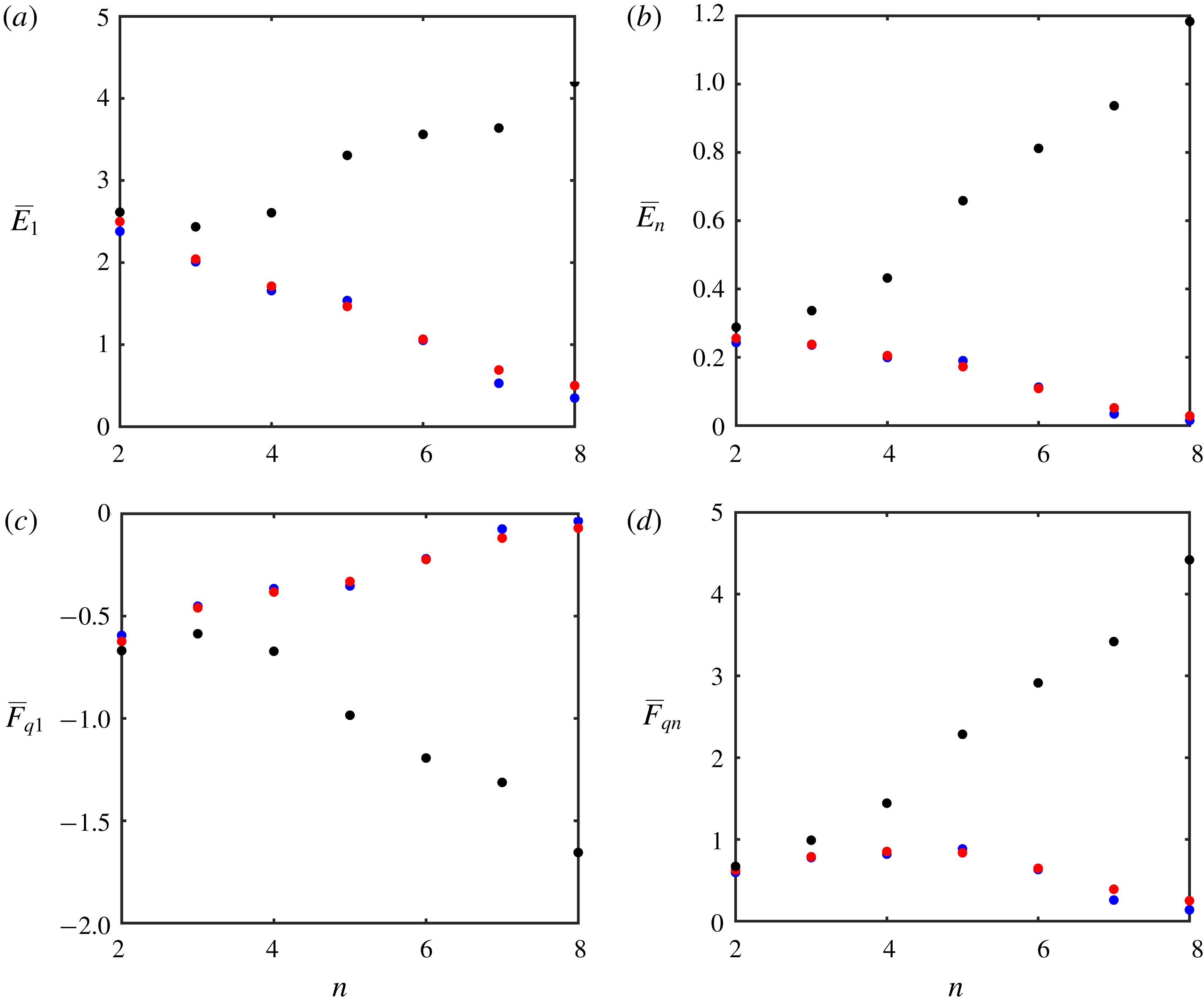
The results in figure 11 reveal very clearly that the influence of submesoscale topography not only persists but substantially grows as the number of layers is increased. In particular, both kinetic energy and PV fluxes systematically decrease with increasing
 $n$
in the non-uniform topography case, whereas the opposite trend is realized in the flat-bottom configuration. As a result, the two systems systematically diverge. For
 $n=8$
, submesoscale topography reduces PV fluxes and energy in all layers by more than an order of magnitude. The fundamentally non-local character of topographic control is truly striking. Even the sub-surface eddying flow in the eight-layer model – which is insulated from the bottom by seven distinct active layers – is drastically slowed down by topographic variability. Another encouraging finding is the quantitative agreement between the original quasi-geostrophic and parametric solutions across a range of stratification patterns (figure 11). The consistency of the full and reduced models is indicative of a very robust mechanism of the submesoscale topographic control of baroclinic instability that can be effectively captured by multiscale methods. This, in turn, raises our hopes of finding analogous solutions in more general and realistic models that go beyond the layered quasi-geostrophic framework.
5 Discussion
This study examines the interaction between mesoscale eddies, topography, and secondary topographically induced submesoscale patterns. We demonstrate that the presence of even weak submesoscale variability in sea-floor depth
 $({\sim}3\,\%)$
has a major impact on the intensity and transport characteristics of baroclinic instability throughout the entire water column. Inspection of the observationally derived bathymetric spectrum (Goff & Jordan Reference Goff and Jordan1988) shows that submesoscale topographic features of such magnitude are expected to be most common in the ocean (appendix A). The ubiquity of submesoscale flow–topography interactions and their profound impact on larger scales of motion motivate efforts to explain the dynamics at play. This task becomes particularly urgent in view of the inability of the current generation of global numerical models to resolve topographic features on the scale of 1–10 km.
The current investigation of processes induced by submesoscale topography employs techniques of multiscale modelling (e.g. Mei & Vernescu Reference Mei and Vernescu2010). One of the key results is the parametric model which expresses the system dynamics entirely in terms of mesoscale variables. This model is successfully validated by comparing its predictions with those generated by corresponding submesoscale-resolving simulations. We demonstrate that the formal requirement of asymptotic scale separation between interacting flow components does not substantially limit the predictive capabilities of the multiscale model. This finding is highly encouraging since the clear-cut separation between mesoscale and submesoscale structures may not be realized in typical oceanic systems. It reinforces our belief that multiscale modelling represents an effective and versatile tool for the analysis and interpretation of a multitude of geophysical phenomena. The dynamic transparency of the multiscale method also makes it possible to physically interpret the chain of processes controlling the inter-scale exchanges in the model. We argue that the feedback of submesoscales on larger scales of motion is initially triggered by the homogenization of potential vorticity in the lowest density layer, which creates a primary submesoscale flow. This primary pattern then nonlinearly interacts with eddies generated by baroclinic instability, which has an adverse effect on mesoscale components and ultimately acts to stabilize the system.
The presented analysis can be extended in a number of promising directions. For instance, the present formulation is based on an idealized harmonic topography, which carries the benefit of analytical tractability and transparency. However, the adoption of more realistic bathymetric patterns, such as afforded by the spectral representation of Goff & Jordan (Reference Goff and Jordan1988), can lead to more quantitative predictions that are directly testable by oceanographic field observations. The problem of parameterizing the influence of complicated multi-harmonic topographic features is challenging and will likely require a major modification of the algorithms used in the present study. However, the recent precedents of applying multiscale methods to irregular realistic patterns in various systems (Radko Reference Radko2016, Reference Radko2019; Radko & Kamenkovich Reference Radko and Kamenkovich2017) suggest that such an approach is potentially viable.
Another natural step in the development of this project is the analysis of more general (e.g. primitive equation) frameworks. The present investigation addressed the dynamics of phenomena contained in the upper-submesoscale range (2.4). This focus made it possible to (i) isolate effects associated with geostrophically balanced motions and (ii) use the quasi-geostrophic framework, which affords a simpler and more transparent view than the one provided by the Navier–Stokes system. In the parameter regime of interest, this restriction has not led to significant dynamical consequences, which was confirmed by comparing quasi-geostrophic solutions with their shallow-water counterparts (appendix B). However, it is desirable to expand the scope of investigation to models which encompass the lower-submesoscale range
 $$\begin{eqnarray}H^{\ast }\ll L_{topogr}^{\ast }\lesssim \frac{U^{\ast }}{f_{0}^{\ast }}.\end{eqnarray}$$
Such analyses would make it possible to address several poorly understood aspects of geophysical turbulence, such as the transition between upscale energy cascade in geostrophic flows and the direct three-dimensional cascade. In this regard, it should be noted that techniques of multiscale modelling are sufficiently generic and could be readily applied to progressively smaller scales and phenomena. It is our belief that the minimal model presented here, interesting as it may be in its own right, offers only a glimpse of insight into the dynamics of the eddying ocean that can be generated by the systematic application of multiscale methods.
Acknowledgements
The author thanks the editor N. Balmforth and the anonymous reviewers for helpful comments. Support of the National Science Foundation (grant OCE 1828843) is gratefully acknowledged.
Appendix A. Analysis of the topographic spectrum
The spectrum of bottom topography for scales of several hundred metres and above is known to be adequately captured by the empirical representation of Goff & Jordan (Reference Goff and Jordan1988),
 $$\begin{eqnarray}P_{h}=\frac{2\unicode[STIX]{x03C0}H_{rms}^{2}(\unicode[STIX]{x1D707}-2)}{k_{0}l_{0}}\left(1+\frac{k_{c}^{2}}{k_{0}^{2}}+\frac{l_{c}^{2}}{l_{0}^{2}}\right)^{-\unicode[STIX]{x1D707}/2},\end{eqnarray}$$
where
 $k_{c}$
and
 $l_{c}$
are the wavenumbers (measured in
 $\text{cycles}~\text{m}^{-1}$
) and
 $H_{rms}^{2}$
is the variance of the topographic height. Nikurashin et al. (Reference Nikurashin, Ferrari, Grisouard and Polzin2014) estimate that typical topographic patterns can be described using the following parameters:
 $$\begin{eqnarray}\unicode[STIX]{x1D707}=3.5,\quad k_{0}=1.8\times 10^{-4}~\text{m}^{-1},\quad l_{0}=1.8\times 10^{-4}~\text{m}^{-1},\quad H_{rms}=305~\text{m}.\end{eqnarray}$$
In the context of our discussion of the effects of submesoscale topography, it is of interest to evaluate the contribution of various spectral components to the net variance of topographic height and, perhaps more importantly, to the variance of the sea-floor slope
 $$\begin{eqnarray}s_{rms}^{2}=\overline{\left(\frac{\unicode[STIX]{x2202}H^{\ast }}{\unicode[STIX]{x2202}x^{\ast }}\right)^{2}+\left(\frac{\unicode[STIX]{x2202}H^{\ast }}{\unicode[STIX]{x2202}y^{\ast }}\right)^{2}},\end{eqnarray}$$
where the overbar represents the spatial average. The counterpart of (A 1) for the spectrum of slope becomes
 $$\begin{eqnarray}P_{h}=\frac{(2\unicode[STIX]{x03C0})^{3}H_{rms}^{2}(\unicode[STIX]{x1D707}-2)}{k_{0}l_{0}}\left(1+\frac{k_{c}^{2}}{k_{0}^{2}}+\frac{l_{c}^{2}}{l_{0}^{2}}\right)^{-\unicode[STIX]{x1D707}/2}\quad (k_{c}^{2}+l_{c}^{2}).\end{eqnarray}$$
A straightforward quantification of different components is readily afforded by the Parseval identity
 $$\begin{eqnarray}h_{rms}^{2}=\iint _{V}P_{h}\,\text{d}k_{c}\,\text{d}l_{c},\quad s_{rms}^{2}=\iint _{V}P_{s}\,\text{d}k_{c}\,\text{d}l_{c},\end{eqnarray}$$
where
 $V$
represents the space of relevant wavenumbers. Of particular interest is the submesoscale component (
 $V_{sm}$
), which we define as a superposition of all spectral harmonics with wavelengths (
 $L_{w}^{\ast }$
) in the following range:
 $$\begin{eqnarray}V_{sm}=\{1~\text{km}<L_{w}^{\ast }<10~\text{km}\}.\end{eqnarray}$$
The large-scale/mesoscale component (
 $V_{lm}$
) is defined accordingly,
 $$\begin{eqnarray}V_{lm}==\{L_{w}^{\ast }>10~\text{km}\},\end{eqnarray}$$
which yields
 $$\begin{eqnarray}\left.\begin{array}{@{}c@{}}h_{sm}^{2}=6.9\times 10^{4}~\text{m}^{2},\quad h_{lm}^{2}=1.7\times 10^{4}~\text{m}^{2},\\ s_{sm}^{2}=0.38,\quad s_{lm}^{2}=3.1\times 10^{-3}.\end{array}\right\}\end{eqnarray}$$
The estimates in (A 8) underscore the potential significance of submesoscale topography in controlling oceanic flows. While the variation in topographic height associated with submesoscale features is comparable to that of larger scales (
 $h_{sm}=263~\text{m}$
,
 $h_{lm}=130~\text{m}$
), the slope is clearly dominated by submesoscale components (
 $s_{sm}=0.61$
,
 $s_{lm}=0.056$
). The latter finding is particularly suggestive since the magnitude of slope appears to be the most germane measure of topographic influences – for instance, topographic effects are reflected in governing equations (2.7) entirely in terms of the slope.
Finally, it is of interest to make a rough assessment of the relative significance of submesoscale topography relative to that of the gradient of planetary vorticity (the beta effect). One of the arguments emphasizing the importance of submesoscale topography is based on the analysis of barotropic potential vorticity,
 $$\begin{eqnarray}Q_{b}=\frac{f^{\ast }+\unicode[STIX]{x1D735}\times \boldsymbol{v}^{\ast }}{H^{\ast }},\end{eqnarray}$$
which is a quasi-conservative quantity that controls several key aspects of ocean dynamics (e.g. Pedlosky Reference Pedlosky1987; Vallis Reference Vallis2006). The meridional gradient of
 $Q_{b}$
reduces, in the limit of weak perturbations, to
 $$\begin{eqnarray}\frac{\unicode[STIX]{x2202}Q_{b}^{\ast }}{\unicode[STIX]{x2202}y^{\ast }}\approx \underbrace{\frac{\unicode[STIX]{x1D6FD}^{\ast }}{H_{0}^{\ast }}}_{a}+\frac{1}{H_{0}^{\ast }}\frac{\unicode[STIX]{x2202}(\unicode[STIX]{x1D735}\times \boldsymbol{v}^{\ast })}{\unicode[STIX]{x2202}y^{\ast }}-\underbrace{\frac{f_{0}^{\ast }}{H_{0}^{\ast 2}}\frac{\unicode[STIX]{x2202}\unicode[STIX]{x1D702}_{b}^{\ast }}{\unicode[STIX]{x2202}y^{\ast }}}_{b},\end{eqnarray}$$
where the term
 $a\,(b)$
measures the influence of the beta effect (topography). The topographic term is separately evaluated for submesoscale components (
 $b_{sm}$
) and for large-scale/mesoscale features (
 $b_{lm}$
) using (A 8), which yields
 $$\begin{eqnarray}a\sim 2.5\times 10^{-15}~\text{m}^{-2}~\text{s}^{-1},\quad b_{sm}\sim 3.8\times 10^{-13}~\text{m}^{-2}~\text{s}^{-1},\quad b_{lm}\sim 3.5\times 10^{-12}~\text{m}^{-2}~\text{s}^{-1}.\end{eqnarray}$$
The result in (A 11) is truly revealing. It shows that submesoscale topographic features contribute to the variability of potential vorticity much more – by almost three orders of magnitude – than does the beta effect. Of course, this estimate should be interpreted with caution since planetary vorticity and topography influence oceanic flows in dynamically dissimilar ways. Therefore, the inequality
 $b_{sm}\gg b_{lm}\gg a$
does not guarantee that submesoscale topography is cardinally more significant than the beta effect or than larger topographic patterns. However, (A 11) draws attention to the apparent bias in the literature toward analyses of large-scale processes in the equilibration of baroclinic instability. It concurrently motivates additional efforts to explain and represent the effects of submesoscale topography, such as the current study strives to offer.
Appendix B. The shallow-water model
The horizontal momentum equations for the two-layer shallow-water Boussinesq system (e.g. Vallis Reference Vallis2006) are given by
 $$\begin{eqnarray}\left.\begin{array}{@{}c@{}}\displaystyle \frac{\unicode[STIX]{x2202}u_{i}^{\ast }}{\unicode[STIX]{x2202}t^{\ast }}+u_{i}^{\ast }\frac{\unicode[STIX]{x2202}u_{i}^{\ast }}{\unicode[STIX]{x2202}x^{\ast }}+v_{i}^{\ast }\frac{\unicode[STIX]{x2202}u_{i}^{\ast }}{\unicode[STIX]{x2202}y^{\ast }}-(f_{0}^{\ast }+\unicode[STIX]{x1D6FD}^{\ast }y^{\ast })v_{i}^{\ast }=-\frac{1}{\unicode[STIX]{x1D70C}_{0}^{\ast }}\frac{\unicode[STIX]{x2202}p_{i}^{\ast }}{\unicode[STIX]{x2202}x^{\ast }}+\unicode[STIX]{x1D708}^{\ast }\unicode[STIX]{x1D6FB}^{2}u_{i}^{\ast }-\unicode[STIX]{x1D6FF}_{i2}\unicode[STIX]{x1D6FE}^{\ast }u_{i}^{\ast },\\ \displaystyle \frac{\unicode[STIX]{x2202}v_{i}^{\ast }}{\unicode[STIX]{x2202}t^{\ast }}+u_{i}^{\ast }\frac{\unicode[STIX]{x2202}v_{i}^{\ast }}{\unicode[STIX]{x2202}x^{\ast }}+v_{i}^{\ast }\frac{\unicode[STIX]{x2202}v_{i}^{\ast }}{\unicode[STIX]{x2202}y^{\ast }}+(f_{0}^{\ast }+\unicode[STIX]{x1D6FD}^{\ast }y^{\ast })u_{i}^{\ast }=-\frac{1}{\unicode[STIX]{x1D70C}_{0}^{\ast }}\frac{\unicode[STIX]{x2202}p_{i}^{\ast }}{\unicode[STIX]{x2202}y^{\ast }}+\unicode[STIX]{x1D708}^{\ast }\unicode[STIX]{x1D6FB}^{2}v_{i}^{\ast }-\unicode[STIX]{x1D6FF}_{i2}\unicode[STIX]{x1D6FE}^{\ast }v_{i}^{\ast },\end{array}\quad i=1,2,\right\}\end{eqnarray}$$
and the layer thickness (
 $h_{i}^{\ast }$
) equations can be written as,
 $$\begin{eqnarray}\frac{\unicode[STIX]{x2202}h_{i}^{\ast }}{\unicode[STIX]{x2202}t^{\ast }}+\frac{\unicode[STIX]{x2202}}{\unicode[STIX]{x2202}x^{\ast }}(u_{i}^{\ast }h_{i}^{\ast })+\frac{\unicode[STIX]{x2202}}{\unicode[STIX]{x2202}y^{\ast }}(v_{i}^{\ast }h_{i}^{\ast })=0.\end{eqnarray}$$
The commonly used rigid lid approximation assumes that the variation in sea-surface height is much less than the variation in thickness of density layers, in which case
 $$\begin{eqnarray}h_{1}^{\ast }+h_{2}^{\ast }=H^{\ast }.\end{eqnarray}$$
The dynamic pressure components (
 $p_{i}^{\ast }$
) in the rigid lid model are also connected in a rather straightforward manner,
 $$\begin{eqnarray}p_{1}^{\ast }=p_{2}^{\ast }+g^{\prime \ast }h_{1}^{\ast }.\end{eqnarray}$$
The governing equations (B 1)–(B 4) are non-dimensionalized using the average ocean depth
 $H_{0}^{\ast }$
as the unit of thickness, the radius of deformation
 $R_{d}^{\ast }=(\sqrt{g^{\prime \ast }H_{0}^{\ast }})/f_{0}^{\ast }$
as the horizontal scale, the nominal speed of the upper layer
 $U^{\ast }$
as the velocity unit and
 $\unicode[STIX]{x1D70C}_{0}^{\ast }U^{\ast 2}$
as the unit of pressure. The non-dimensional system takes the following form:
 $$\begin{eqnarray}\left.\begin{array}{@{}c@{}}\displaystyle \frac{\unicode[STIX]{x2202}u_{i}}{\unicode[STIX]{x2202}t}=-\frac{\unicode[STIX]{x2202}p_{i}}{\unicode[STIX]{x2202}x}+G_{ui},\quad G_{ui}=-u_{i}\frac{\unicode[STIX]{x2202}u_{i}}{\unicode[STIX]{x2202}x}-v_{i}\frac{\unicode[STIX]{x2202}u_{i}}{\unicode[STIX]{x2202}y}+(Ro_{R}^{-1}+\unicode[STIX]{x1D6FD}y)v_{i}+\unicode[STIX]{x1D708}\unicode[STIX]{x1D6FB}^{2}u_{i}-\unicode[STIX]{x1D6FF}_{i2}\unicode[STIX]{x1D6FE}u_{i},\\ \displaystyle \frac{\unicode[STIX]{x2202}v_{i}}{\unicode[STIX]{x2202}t}=-\frac{\unicode[STIX]{x2202}p_{i}}{\unicode[STIX]{x2202}y}+G_{vi},\quad G_{vi}=-u_{i}\frac{\unicode[STIX]{x2202}v_{i}}{\unicode[STIX]{x2202}x}-v_{i}\frac{\unicode[STIX]{x2202}v_{i}}{\unicode[STIX]{x2202}y}-(Ro_{R}^{-1}+\unicode[STIX]{x1D6FD}y)u_{i}+\unicode[STIX]{x1D708}\unicode[STIX]{x1D6FB}^{2}v_{i}-\unicode[STIX]{x1D6FF}_{i2}\unicode[STIX]{x1D6FE}v_{i},\\ \displaystyle \frac{\unicode[STIX]{x2202}h_{i}}{\unicode[STIX]{x2202}t}=G_{hi},\quad G_{hi}=-\frac{\unicode[STIX]{x2202}}{\unicode[STIX]{x2202}x}(u_{i}h_{i})-\frac{\unicode[STIX]{x2202}}{\unicode[STIX]{x2202}y}(v_{i}h_{i}),\\ \displaystyle h_{1}+h_{2}=H=1+\hat{\unicode[STIX]{x1D702}},\quad \hat{\unicode[STIX]{x1D702}}=\frac{\unicode[STIX]{x1D702}_{b}^{\ast }}{H_{0}^{\ast }},\\ \displaystyle p_{1}=p_{2}+\frac{h_{1}}{Ro_{R}^{2}},\quad Ro_{R}=\frac{U^{\ast }}{f_{0}^{\ast }R_{d}^{\ast }},\quad \unicode[STIX]{x1D6FD}=\frac{\unicode[STIX]{x1D6FD}^{\ast }R_{d}^{\ast 2}}{U^{\ast }},\quad \unicode[STIX]{x1D708}=\frac{\unicode[STIX]{x1D708}^{\ast }}{R_{d}^{\ast }U^{\ast }},\quad \unicode[STIX]{x1D6FE}=\frac{\unicode[STIX]{x1D6FE}^{\ast }R_{d}^{\ast }}{U^{\ast }}.\end{array}\right\}\end{eqnarray}$$
The upper layer dynamical pressure can be inferred from the instantaneous distribution of
 $(u_{i},v_{i})$
using the diagnostic equation
 $$\begin{eqnarray}\displaystyle & & \displaystyle \frac{\unicode[STIX]{x2202}}{\unicode[STIX]{x2202}x}\left(H\frac{\unicode[STIX]{x2202}p_{1}}{\unicode[STIX]{x2202}x}\right)+\frac{\unicode[STIX]{x2202}}{\unicode[STIX]{x2202}y}\left(H\frac{\unicode[STIX]{x2202}p_{1}}{\unicode[STIX]{x2202}y}\right)=\frac{\unicode[STIX]{x2202}}{\unicode[STIX]{x2202}x}\left(h_{1}G_{u1}+u_{1}G_{h1}+h_{2}G_{u2}+u_{2}G_{h2}+\frac{h_{2}}{Ro^{2}}\frac{\unicode[STIX]{x2202}h_{1}}{\unicode[STIX]{x2202}x}\right)\nonumber\\ \displaystyle & & \displaystyle \quad +\,\frac{\unicode[STIX]{x2202}}{\unicode[STIX]{x2202}y}\left(h_{1}G_{v1}+v_{1}G_{h1}+h_{2}G_{v2}+v_{2}G_{h2}+\frac{h_{2}}{Ro^{2}}\frac{\unicode[STIX]{x2202}h_{1}}{\unicode[STIX]{x2202}y}\right),\end{eqnarray}$$
which is iteratively solved for
 $p_{1}$
using the generalized minimum residual method.
The major complication in integrating the shallow-water equations using spectral methods is that periodic boundary conditions, which were conveniently applied to perturbation fields in the quasi-geostrophic model, can no longer be employed in the meridional
 $(y)$
direction. This complication is addressed by using
 $\cos (\unicode[STIX]{x03C0}n_{y}yL_{y}^{-1})$
functions
 $(n_{y}=0,1,\ldots ,N_{y}-1)$
for
 $(h_{i},p_{i},u_{i})$
and
 $\sin (\unicode[STIX]{x03C0}n_{y}yL_{y}^{-1})$
for
 $v_{i}$
. Such a choice implies that the flow field satisfies the rigid no-stress boundary conditions at
 $y=0,L_{y}$
. However, in
 $x$
-direction we still use a full Fourier series, which conforms to periodic boundary conditions. In order to maintain the mean vertical shear indefinitely, the
 $x$
-averaged zonal velocity is weakly relaxed to the following target distribution:
 $$\begin{eqnarray}\overline{u}_{1}=\tanh (10\sin ^{2}(\unicode[STIX]{x03C0}yL_{y})),\quad \overline{u}_{2}=0.\end{eqnarray}$$
The implementation of the relaxation algorithm is particularly straightforward in the context of our spectral model, where
 $x$
-averages are represented by the Fourier harmonics with zero horizontal wavenumbers
 $(k_{x}=0)$
. The target velocity pattern (B 7) is shown in figure 12(a). In most of the computational domain
 $\overline{u}_{1}\approx 1$
. However,
 $\overline{u}_{1}$
gradually reduces to zero within the narrow meridional boundary layers, which makes it possible to satisfy the boundary conditions
 $\unicode[STIX]{x2202}h_{i}/\unicode[STIX]{x2202}y=0,v_{i}=0$
implicitly imposed by the spectral model at
 $y=0,L_{y}$
.
The shallow-water model. The upper layer zonal velocity of the background flow is shown in (a). Panels (b,c) present the instantaneous patterns of zonal and meridional velocities in the quasi-equilibrium phase (
 $t=500$
) of the simulation with meridional topography. Dashed lines mark the central region that is used to evaluate the equilibrium values of energy and PV flux. The potential vorticity anomalies in the central regions of the top and bottom layers are shown in (d) and (e) respectively.

The model was initialized by the geostrophically balanced basic state
 $(\overline{u}_{i},\overline{h}_{i})$
, conforming to the target velocity distribution (B 7), which was slightly augmented by random low-amplitude perturbation and then integrated in time. The shallow-water simulations are computationally more intensive than their quasi-geostrophic counterparts. Severe limitations on time step in the shallow-water model are imposed by the requirement to resolve relatively fast interfacial internal waves that are filtered out by the quasi-geostrophic approximation (§ 2). This makes it difficult to achieve the same resolution as afforded by the quasi-geostrophic model. Therefore, the following shallow-water experiments resolved the computational domain of
 $L_{x}\times L_{y}=15\times 30$
by
 $N_{x}\times N_{y}=384\times 768$
grid points. Nevertheless, this discretization adequately represents topographic variability for
 $d=0.5$
, and typical flow patterns realized in the shallow-water simulations are shown in figure 12. As in their quasi-geostrophic counterparts, the velocity fields are dominated by active mesoscale variability (figure 12
b,c).
To offer more quantitative comparisons, we focus on the central region of the computational domain
 $$\begin{eqnarray}{\textstyle \frac{1}{4}}L_{y}<y<{\textstyle \frac{3}{4}}L_{y},\end{eqnarray}$$
where the flow is not strongly affected by rigid meridional boundary conditions. In particular, we evaluate the equilibrium levels of kinetic energy
 $\overline{E}_{i}$
(
 $i=1,2$
) and the potential vorticity flux in the upper layer
 $(\overline{F}_{q1})$
averaged over region (B 8). To be consistent with the definition of PV anomaly adopted in our quasi-geostrophic model (2.8), we introduce the corresponding diagnostic variable for the shallow-water system,
 $$\begin{eqnarray}q_{i}=\left(\frac{f+\unicode[STIX]{x1D735}\times \boldsymbol{v}_{i}}{h_{i}}-\frac{f}{\overline{h}_{i}}\right)\overline{\overline{h}}_{i},\end{eqnarray}$$
where
 $\overline{\overline{h}}_{i}$
is the mean basic thickness (
 $\overline{h}_{i}$
) in the area (B 8). The typical distribution of PV anomalies (e.g. figure 12
d,e) is structurally similar to patterns realized in quasi-geostrophic experiments (cf. figure 3
a,b). In all cases, the upper layer flow field is dominated by intense mesoscale variability whereas the lower layer PV anomaly also reveals a clear imprint of the bottom topography.
A series of experiments analogous to that in figure 12 were performed for various values of the orientation variable (
 $\unicode[STIX]{x1D703}$
). The resulting equilibrium values of
 $(\overline{E}_{1},\overline{E}_{2},\overline{F}_{q1})$
averaged over the central area (B 8) are plotted in figure 9 along with the corresponding quasi-geostrophic results, revealing their general consistency. In both models, the intensity of baroclinic instability monotonically increases (decreases) as the topography becomes more meridional (zonal). Some quantitative differences are apparent in the energy and PV flux estimates offered by quasi-geostrophic and shallow-water models. However, these differences do not seem to reflect any systematic trends. Furthermore, it is likely that they are caused by dissimilar meridional boundary conditions rather than by inherently non-quasi-geostrophic effects in the shallow-water system.