The Great Depression was a cataclysmic event in U.S. history. The downturn rippled through all aspects of society, including the institution of marriage: marriage rates fell by 20 percent from 1929 to 1933. This article examines whether the economic collapse actually caused the lower levels of marriage or whether the decline in marriage rates was an unrelated trend. The evidence suggests that it was the former: marriage propensities and gross domestic product (GDP) are positively correlated throughout the time period and at different levels of geographic aggregation. The relationship is robust to controlling for other variables, including place and time fixed effects. During the tumultuous 1930s, marriage rates fell most in places where the Depression hit hardest, and marriage rates recovered where the economy rebounded. Economic conditions specifically linked to the suitability of males for marriage are the strongest predictors of women's marriage probabilities. In addition to the immediate impact of the downturn on marriage, the Great Depression had a long-term effect on the marriages made in the time period. Marriages formed in poor economic times were more likely to survive than marriages made in more affluent periods, suggesting that individuals who married in lean economic periods were perhaps better matched or their initial exposure to hardship during their courtship forged strong bonds.
Through what channel does the economy affect marriage? In the Becker model of marriage (Becker Reference Becker1981), the gains to marriage come through specialization, where women specialize in home production and men specialize in market production.Footnote 1 In the Becker model, single women marry if the gains to marriage are greater than her outside option (current income). Economic downturns may then decrease the marriage rate by lowering male employment rates and thus reducing the number of marriageable men (men able to specialize in the market production). However, economic downturns may actually increase the marriage rate if they decrease the value of the outside option: employment prospects for single women. Therefore, when a significant number of single women participate in the labor force (as was the case in the 1930s (Goldin Reference Cvrcek1990)), the effect of the economy on marriage could be ambiguous. I show that labor markets in the 1930s exhibit the predicted effects on marriage: robust male labor markets have a positive effect while robust female labor markets have a negative one. Overall, the male labor market effect dominates and a positive correlation between marriage and the economy is observed.
Several scholars have examined the relationship between economic conditions and marriage. Much of the work has focused on the late twentieth century. Francine Blau, Lawrence M. Kahn, and Jane Waldfogel (Reference Blau, Kahn and Waldfogel2000) and Robert Wood (Reference Wood1995) use microlevel data on individuals to estimate the extent to which deteriorating labor market opportunities can explain the retreat from marriage observed among lower income groups. Other research has highlighted the role of female labor conditions (Bitler et al. Reference Bitler, Gelbach, Hoynes and Zavodny2004) and male relative income (Watson and McLanahan Reference Watson and McLanahan2011; Loughran Reference Loughran2002). Historically, there is ample evidence that the economy affected marriage. Robust early colonial economies and economic booms and busts of the late nineteenth century and early twentieth century have been related to both the propensity to marry and age at marriage (Haines Reference Haines1996; Fitch and Ruggles Reference Fitch, Ruggles. and Waite2000; Cvrcek Reference Cvrcek2012). This article adds to the existing literature by examining factors that have concerned scholars of recent marriage trends in the context of the 1930s.
I exploit the variation in economic conditions engendered by the Great Depression to estimate the effect of local GDP on the probability of marriage for young women and men. Specifically, I perform three analyses dictated by geographic and temporal constraints. State income data and manufacturing data are available for the period from 1920 to 1939; thus, at the state level I am able to estimate the effect of state income and earnings variation on individuals’ marriage decisions throughout the entire Depression (1929–1939) and the interwar period (1920–1939). Retail sales per capita is available semi-annually from 1929 to 1939 at the county level, allowing me to estimate the effect of economic factors within county groups (categorized by the census as state economic areas, hereafter SEAs) on marriage decisions for select years from 1929 to 1939. Finally, detailed county information exists for 1940. I use this information to understand how sex ratios, male and female unemployment, and local GDP affected the stock of marriages in 1940. In general, I find that local GDP (proxied by state income per capita or SEA/county retail sales per capita) is positively correlated with the probability of marriage. Male employment opportunities (measured by manufacturing earnings per worker or male unemployment) are also positively correlated with marriage probabilities. Additionally, there is some evidence that female labor market opportunities are negatively correlated with marriage.
In the long run, the Great Depression had little impact on marriage rates; however, it did affect the quality of matches. Marriage rates fell at the onset of the Depression but recovered quickly when the economy rebounded. The result was that marriages were delayed rather than denied. Members of the cohort who came of age in the Great Depression were no more likely to never marry than members of subsequent or preceding cohorts. The long-run effect of the Great Depression was on marriage stability; couples married during the economic doldrums were less likely to divorce. These couples may have been matched well on qualities other than short-term economic prospects and therefore their marriages were less susceptible to divorce in the long term. Another possible explanation is that the exposure to the Depression during their initial years of courtship forged a strong bond that enabled couples to weather subsequent hardship.
TRENDS
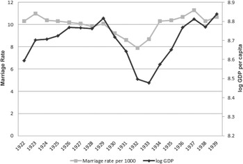
In order to place the Depression era in context, I report the long-run trends in GDP and marriage rates in the United States. Prior to 1960, there was a positive relationship between GDP and marriage rates at the national level. Figure 1, a scatter plot of marriage rates and de-trended log GDP per capita in the United States from 1887 to 1960, shows the positive relationship. The trend line is upward sloping with above-trend GDP years corresponding to years with higher marriage rates. After 1960, marriage rates and de-trended log GDP per capita evidence a weaker relationship (results not shown); this fact is perhaps not surprising given there is little debate that many of the factors driving the marriage decision changed after 1960.Footnote 2 Figure 2, a plot of marriage rates and log GDP per capita from 1920 to 1940, demonstrates that the correlation between log GDP per capita and marriage rates was particularly strong in the interwar period. Marriage rates remain steady during the 1920s and then fall after the onset of the Depression, but rebound when the economy begins to recover in 1934.
MARRIAGE RATES AND DETRENDED GDP PER CAPITA (1887–1960, WWI AND WWII EXCLUDED)

MARRIAGE RATES AND LOG GDP PER CAPITA (1922–1939)

Evidence on the percentage of women never married and on the age of first marriage suggests that there were 230,000 fewer marriages in 1931 and 1932 compared with 1930, but that these marriages were delayed rather than denied. Women who attained marriageable age during the economic doldrums of the Great Depression were actually less likely to never marry than women who came of age during the roaring 1920s: by 1960, 6.8 percent of women born between 1912 and 1915 had never been married, while 8.3 percent of women born from 1902 to 1905 had never been married.Footnote 3 Age at first marriage for women stayed fairly constant from 1921 until 1932, hovering around 21.4 before increasing to a high of 21.8 by 1935, then it returned to its pre-Depression level in 1938 and remained at that level until 1940.Footnote 4 The rise in age at first marriage from 1932 to 1935 is consistent with marriage delay. If some of the women who did not marry during the marriage downturn of 1930–1933 married in the recovery period from 1933–1937, then these women would be a few years older and would thus push the average marriage age from 1934–1937 upwards (provided marriage rates for women aging into the marriage pool were similar to pre-Depression marriage rates). Thus, the aggregate trends suggest that the impact of the economic downturn on marriage rates was not permanent.
Qualitative primary sources echo the trends observed at the national level: women postponed marriage during the downturn. They delayed for a number reasons related to local economic conditions. Women in Chicago families interviewed by Ruth Cavan and Katherine Ranck explained, “The boys have no jobs,” and “I want a man with a job.”Footnote 5 A mother, wary of losing her working daughter's income, relayed, “I hope she will not marry for two years as the family needs her help.” Falling incomes in general also took their toll on marriage. A woman in the Chicago study has a boyfriend, but they must delay marriage until “he can support her.” Men in the sample complain about barely being able to cover their own expenses, let alone support a wife. An Oakland study conducted by Glen H. Elder, Jr. yields similar experiences: widespread delay among his sample of men and women. Young Oakland women blame financial constraints for their inability to entice desirable men, noting they could not afford nice dresses or keep up proper grooming habits. At the same time, young Oakland men had difficulty finding jobs and affording courtships.Footnote 6
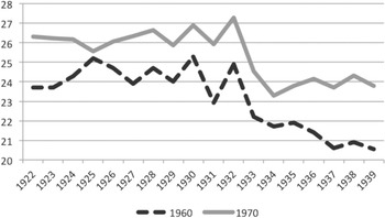
Were the marriages formed in the Great Depression different than those formed in times of prosperity on any other dimension? Long-run divorce trends suggest marriages forged in the hard times of the Great Depression were less likely to be dissolved than marriages that began in other time periods. Figure 3 shows the percent of persons by marriage year cohort who did not remain in their first marriage by 1960 and 1970.Footnote 7 Individuals whose marriage occurred in 1933 or after were more likely to still be in that relationship in 1960 and 1970 than those married before 1932.
PERCENT OF INDIVIDUALS NOT IN THEIR FIRST MARRIAGE IN 1960 AND 1970 BY MARRIAGE YEAR

The aggregate time series and the primary sources suggest a positive relationship between GDP and marriage, but neither is conclusive. The primary sources are taken from a small subsample of people and therefore are not representative of the national experience. And while the aggregate patterns demonstrate a correlation between GDP and marriage, microeconomic data are needed to more firmly link marriage decisions to GDP and to identify the key economic variables that influence the marriage decision. Furthermore, microeconomic data can be used to establish the long-run effects of the Great Depression on marriage, in other words, were marriages formed during periods of hardship more likely to endure than those formed in boom times?
CONCEPTUAL FRAMEWORK
I provide a brief theoretical framework outlining how local economic conditions might affect an individual's propensity to marry. In the typical matching models first introduced by Dale Mortenson (Reference Mortensen1982) and applied to marriage by Ken Burdett and Melvyn G. Coles (Reference Burdett and Melvyn1997), potential spouses arrive at a rate α. Each spouse is drawn from a distribution F(z), where z denotes a measure of quality. A match is accepted if the potential spouse has a z-value greater than an individual's reservation value, z∗ . Once a match is accepted, the couple exits the marriage market, and divorce is not an option. Given the low rates of divorce in the period, this assumption is not as unrealistic as it might be in more recent periods.Footnote 8 Empirically, this framework suggests one should observe relationships between the sex ratio and marriage, and between local GDP and marriage. An increase in sex ratio (total men/total women) affects the propensity to marry by lowering α for men and increasing α for women. GDP should increase marriage rates because higher GDP is associated with higher male earnings/employment and is thus a proxy for the quality of males. In areas with higher GDP, the distribution of male quality F(z) will be shifted upward and there will be more men above the women's reservation value of z∗ . It is through this mechanism that lower GDP will induce fewer marriages.
Now consider the same theoretical model with an added dimension: compatibility. Each potential spouse's quality (z) consists of two components, i and q, drawn from distributions F(i) and F(q), respectively, where i denotes a potential spouse's lifetime income and q denotes compatibility. Compatibility is defined as the lifetime utility derived from time spent with one's spouse. For instance, an abusive husband would have a low value of q. Assume that a spouse is accepted when z, where z = i + q, is greater than the reservation value z∗ , and z∗ is time invariant. Thus, in periods of economic hardship when F(i) is shifted downward, the marriages observed will consist, on average, of husbands with higher q values than husbands observed during prosperous times. If q is associated with marriage longevity, then marriages formed during economic hardship should last longer on average, that is, be less susceptible to divorce than those formed during economic prosperity.
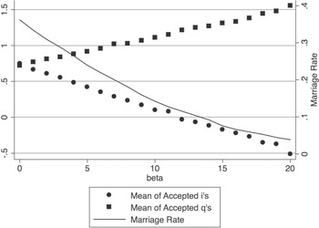
Figure 4 shows the results of a simple simulation that demonstrates how the distribution of accepted men evolves as F(i) shifts downward. In this simulation F(i) is normal N(0-β,1), where β represents the severity of the economic shock: the larger β, the further F(i) is shifted to the left. The distribution, F(q), is normal N(0,1). Each man receives a draw from F(i) and F(q). A woman meets one man; she marries this man if i + q > 0.5. I plot the mean of the accepted men's q values and i values as β increases. I also plot the percentage of men accepted on the secondary axis; the percentage of men accepted decreases as the economic shock β increases. The figure shows that the mean of accepted men's q values increases with the negative economic shock to men's income distribution, F(i), while the mean of the accepted men's i value exhibits a negative relationship with β. This simple simulation suggests that as an economy worsens, marriage rates will decrease and the marriages formed will consist of men with lower incomes but higher match compatibility (q).
DISTRIBUTION MEANS AND MARRIAGE RATES SIMULATION

DATA
I use individual data from the decennial U.S. censuses of 1930, 1940, and 1950 and then merge these data with local economic data from the place in which an individual lived during her marriageable years; the end result is a dataset that reflects the economic conditions a woman faced during her at-risk for marriage years. For the bulk of the empirical analysis, I ascertain an individual's marriage year and then build multiple annual observations from their single census observation to represent her marriageable years. I limit the sample to women because the majority of the decennial censuses contain marriage data only for women, and because the conceptual framework suggests women have agency in the decision to marry.Footnote 9 In the constructed data, a woman's first observation occurs in the year she turns 17. Then there is an observation for each subsequent year until the woman marries or turns 28. I chose the age limits of 17 to 28 because more than 80 percent of first marriages occur in those years, and the decision-making process for choosing a spouse should be consistent across those ages.Footnote 10 I then merge this constructed panel data with economic conditions in each year for which data is available.
The constructed retrospective marriage histories have several advantages over conventional state counts of marriages. Firstly, the retrospective marriage histories are more detailed because they are observed at the individual level. This allows me to control for important confounding factors in the marriage decision, such as race, education level, and age. Secondly, the retrospective marriage histories are potentially more accurate than the raw marriage rates that are based on marriage license data. In a recent study, Rebecca M. Blank, Kerwin Kofi Charles, and James Sallee (Reference Blank, Charles and Sallee2009) found retrospective marriage histories to be a more accurate representation of where and at what age a person married because data from marriage licenses were prone to errors due to individuals circumventing the minimum age at marriage laws by misreporting or by traveling to a more lenient state for marriage.
Sources of Local Economic Data
State income data exist for the entire interwar period. The income data are from the Bureau of Economic Analysis (BEA) for the years 1929–1938. Before 1929, the data come from John Martin and Robert Nathan (1939) as adjusted by Price Fishback.Footnote 11 Data on manufacturing are also available at the state level for the odd years from 1919 to 1939 from the censuses of manufacturing. At the county level, Fishback, Horrace, and Kantor (Reference Fishback, Horrace and Kantor2005) compiled a detailed panel data set for the 1930s. This data set includes retail sales per capita for the years 1929, 1933, 1935, and 1939.Footnote 12 No income data exist for the Great Depression at the county level; therefore, this retail sales variable is my proxy for local macroeconomic activity. Fishback, et al. (Reference Fishback, Horrace and Kantor2005) found annual national aggregates of retail sales to have correlations above 0.99 with total personal expenditures for the time period 1929 to 1969. Within the Great Depression, Fishback, et al. (Reference Fishback, Horrace and Kantor2005) show correlations between retail sales and state level per capita income to be 0.87, 0.89, 0.88, and 0.90 for the years that the retail sales variable was available. At the county level, in addition to retail sales, semi-annual data exist for manufacturing earnings and manufacturing value added. For counties where manufacturing is an important part of the economy, manufacturing earnings will be a plausible proxy for local labor market conditions. The Fishback data set also contains many more characteristics at the county level for the decennial years of 1930 and 1940, including potentially important factors for marriage such as unemployment and sex ratios.
Marriage Year and Marriage Location
From the census questions about marriage, I ascertain an individual's probable marriage year. Calculation of a marriage year is complicated by the fact that the census marriage variables (age of marriage for the 1930 and 1940 censuses, duration of current marital status for the 1950 census) are recorded as discrete variables when these variables are continuous. For instance, if an individual reported being married for two years in 1950, depending on the month of marriage, the marriage could have occurred exactly 2.0 years ago (which would correspond to a marriage year of 1948) or it could have occurred up to 2.99 years ago (which would correspond to a marriage year of 1947). Each census contains slightly different information on marriage, and given the relevant information in each census, multiple marriage years are possible. I assign women to all their possible marriage years. I then weight the possible marriage years with the probability that the marriage occurred in that year as determined by the distribution of marriage months, distribution of birth months, current age gap with spouse, and age at marriage gap with spouse.
My empirical strategy relies on locating women from the U.S. census in the place where they lived at the time of marriage. The geographic levels in the empirical analysis are state and SEA. The information from the U.S. census available for placing women at the state level is current state, state of birth, spouse's state of birth, and state of birth of eldest child living in the household.Footnote 13 From the four state data points (current state, birth state, spouse's birth state, and eldest child's birth state), I can construct a probable marriage state. I then assume that a woman lived in this state for the years leading up to her marriage. More than 80 percent of the sample has an agreement on at least three of those locations, or two if childless. For the remaining 20 percent, I duplicate the observation and assign one observation to the birth state and one observation to the current state and then give each observation half weight.Footnote 14
There is less information available for placing women at the SEA level. The 1940 census has current SEA and SEA five years prior (1935) and spouse's current SEA and 1935 SEA. I assume people lived in their 1935 SEA for the years prior to 1935. For those with the same current and past SEA, I assume they lived in that SEA for the whole period. For those who switched SEAs from 1935 to 1940 and did not marry, I assign a random move year. For those who do marry, if they and their spouse had the same 1935 SEA, I assume they married in the 1935 SEA and then moved together to the new 1940 SEA. Therefore, the old SEA is assigned to the marriage year and all years prior. In the case where an individual's spouse lived in the 1940 SEA in 1935, I assume that individual moved to the new SEA, met her spouse, and married. In these cases, the new SEA is assigned to the marriage year. For individuals from the 1950 census, only the 1950 and 1949 SEA are available; I assume the individual lived in the 1949 SEA for the years of analysis: 1929–1939.
My assignments of women to SEA might introduce migration bias from women who move before 1935. The first type of bias would be misplacement of a woman during her single years. For instance, consider a woman who moves from a low GDP SEA to a high GDP SEA in 1933 and then marries a man she met from her new SEA in 1934. I would incorrectly record her as unmarried in the new high GDP SEA from 1929 to 1933 when she was actually unmarried in her old low GDP SEA. A wrong assignment of this type would bias the estimate of the local GDP effect downward. Conversely, migration from a high GDP SEA to a low GDP SEA would bias the coefficient on GDP upward. A second type of bias will be misallocation of the place of marriage SEA for married movers. This will occur when a woman marries in one SEA prior to 1935 and then moves with her husband to another SEA prior to 1935. In these cases, misallocation of women who move from low GDP SEAs to high GDP SEAs will lead me to conclude there exists a relationship between GDP and marriage when none is present. To summarize, positive bias in the estimated effect of the economic conditions on marriage will stem from single women moving from high to low GDP SEAs who then marry, and married women moving from low to high GDP SEAs. Negative bias will arise from single women moving from low to high GDP SEAs who then marry, and married women moving from high to low GDP SEAs.
I analyzed the migration patterns for individuals from 1935 to 1940 for my population of interest (women age 17–35) to understand the extent of the possible migration bias from 1930 to 1935. The two groups that might cause bias are married movers and single movers who then marry. I found that 52 percent of moves amongst these two groups would produce negative bias, while 48 percent would produce positive bias. Thus, if migration patterns were similar from 1930 to 1935, the net effect would be to downwardly bias the estimated effect of local economic conditions on marriage.
EMPIRICAL FRAMEWORK AND RESULTS
State Level
I begin by examining the effect of a state's economic performance on a woman's probability of marriage in the Great Depression. State income data is available annually from 1919 to 1940, and manufacturing data is available for every other year from 1921–1940.Footnote 15 Utilizing the retrospective marriage histories generated from the 1940 and 1950 censuses, I estimate a linear probability model of marriage:

where Mijt is a dummy equal to 1 if individual i in state j was married in year t, αj is a state fixed effect, yeart is a year fixed effect, xi is a vector of individual characteristics that may impact the marriage decision (includes: age, age squared, race, urban status, census year, and education (where available)), and yjt is a vector of state economic variables in year t. The state fixed effect controls for any time invariant differences between states in their marriage propensity, while the year fixed effect controls for any nationwide time trends. The vector of the coefficients of interest γ, the effects of a state's economic characteristics on the marriage probability, is identified by economic changes within a state over time. Year and state fixed effects can account for almost 95 percent of the variation in state incomes; therefore, I estimate the equation without year fixed effects as well.
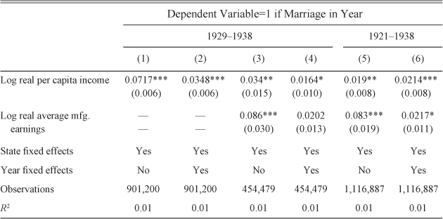
THE EFFECT OF ECONOMIC CONDITIONS ON MARRIAGE (STATE LEVEL)

∗ = Significant at the 10 percent level.
∗ = Significant at 5 percent level.
∗∗∗ = Significant at 1 percent level.
Notes:
Standard errors (in parentheses) are clustered by year and state. Other controls: age, age squared, dummy if in metropolitan area, race, and census year dummy. Sample includes women age 17–27. Income data is available for the entire time period, while manufacturing data is only available for the odd years.
Source:
Author's calculations.
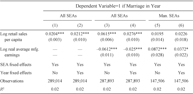
THE EFFECT OF ECONOMIC CONDITIONS ON MARRIAGE 1929, 1933, 1935, 1939 (SEA LEVEL)

∗ = Significant at the 10 percent level.
∗ = Significant at 5 percent level.
∗∗∗ = Significant at 1 percent level.
Notes:
Standard errors (in parentheses) are clustered by year and SEA. Other controls: age, age squared, dummy if in metropolitan area, education, race, and census year dummy. Sample includes women age 17–27.
Source:
Author's calculations.
Table 1, which reports the results of estimating equation (1), shows that state economic conditions had a positive effect on a woman's probability of marriage. The baseline estimate from column (1) suggests that a 10 percent increase in state income would raise a women's probability of marriage by 0.7 percentage points, a 7 percent increase in the probability of marriage in a given year. In my preferred specification with year fixed effects, column (2), the estimated coefficient on income per capita is lowered to 0.0348 but remains statistically significant at the 1 percent level. In columns (3)–(4) real manufacturing earnings are added to the specification. The estimated effect of state income remains statistically significant at conventional levels. However, log average manufacturing earnings exhibits a larger impact on the marriage probability. Average manufacturing earnings is perhaps a better predictor for the probability of marriage than real per capita income because while real per capita income reflects the health of the overall economy, manufacturing earnings are an indicator of the prospects and marriageability of young men. The estimated effect of manufacturing earnings in column (4) suggests a 10 percent increase would increase the probability of marriage by 0.2 percentage points, a 2 percent increase (though the coefficient is not statistically distinguishable from zero at conventional levels). In columns (5) and (6), I estimate the effect of economic variables on marriage over the entire period, from 1921 to 1938. The estimates are comparable to those using only the Depression years, suggesting that the economy influenced marriage over the whole interwar period and not only during the 1930s. The estimated effects of manufacturing earnings are larger than the effects of state income in columns (5) and (6), although the estimates are not statistically different from each other when year fixed effects are included in column (6). The estimates from column (6) suggest that the average decrease in state incomes from 1929 to 1932 ($356 per capita, an average 28 percent decline) would have lowered the probability of a woman marrying by 6 percent (a 0.6 percentage point decline).
State Economic Area Level
Table 2 shows the results of estimating equation (1) at the SEA level. From 1950 onwards, only select counties are available in public-use micro-data. The lowest level of geographic identification is SEAs, which are groups of counties. As detailed in the data section, I aggregated up the county level data to the SEA level and merged this information with retrospective marriage histories constructed from the 1940 and 1950 census. The baseline estimated effect of GDP (proxied by retail sales per capita) in column (1) suggests that a 38 percent decrease (the average drop in retail sales per capita from 1929 to 1932) would decrease the probability of marriage by 0.8 percentage points, an 8 percent decrease. The coefficient does not statistically significantly change when year fixed effects are added in column (2). In column (3), I include log average manufacturing earnings per manufacturing employee. In these specifications, retail sales per capita positively impacts marriage, but manufacturing earnings have the opposite of the expected effect: they negatively impact marriage. However, manufacturing may not be an important component of many SEA's economies. In columns (5) and (6), I limit the sample to SEAs with above the median number of manufacturing establishments. In these SEAs, where one would expect manufacturing to be an important part of the local economy, I find that manufacturing earnings do positively influence the probability of marriage. The estimates from column (6) suggest that a 30 percent decline in earnings per capita (the average change from 1929 to 1933) would lower the probability of marriage by 1 percentage point, a 10 percent decrease. The results in columns (5) and (6) echo the findings from the state level specification, in that manufacturing earnings are a stronger predictor of marriage than the income proxy variable.
SEA Level 1940
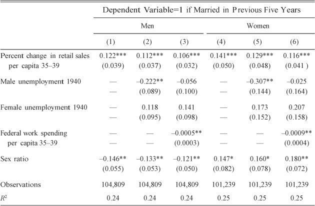
In this section, I examine the effect of local economic conditions in 1940 on the probability an individual had married in the previous five years. For the year 1940, there exist many more local economic variables than I have used in the preceding sections, where I was limited to variables available on a semi-annual basis.Footnote 16 Table 3, shows the estimated effect of various local economic characteristics on the probability a man or woman who was single in 1935 married in the subsequent five years. The estimates in columns (1) and (2) suggest that men and women in SEAs that experienced more growth in retail sales per capita from 1935 to 1940 were more likely to marry than their counterparts in low growth SEAs. A 10 percent increase in retail sales per capita increased the probability of marriage by 5 percent for men and 4 percent for women. The sex ratio in 1940 is defined as white males 21–40 divided by white females 21–40. In concordance with standard marriage market theory, the estimates suggest that a higher number of males relative to females increased marriage probabilities for women and decreased marriage probabilities for men. In columns (2) and (4), I include unemployment rates in 1940. Under the assumption that unemployment in 1940 is a proxy for unemployment in the previous five years, the results imply that male unemployment negatively impacted the probability of marriage while female unemployment positively impacted marriage, albeit not statistically significantly.Footnote 17 It is feasible that male and female unemployment would have dichotomous effects on marriage. High female unemployment might drive women who have little outside economic support to marry. High male unemployment shrinks the pool of marriageable men and lowers marriage probabilities. Specifically, I find that a 5 percent increase in male unemployment (a standard deviation) lowered men and women's marriage probabilities by around 4 percent. In columns (3) and (6), I add total per capita spending by the Works Progress Administration (WPA) to the specification. The WPA started in July 1935 and the data source ended in June 1939; thus, total WPA spending accurately reflects work relief spending for the period in question. The estimates show that WPA spending per capita is negatively associated with the probability of marriage. It is not necessarily the case that there is a causal link between WPA spending and marriage. The coefficient on the effect of male unemployment becomes statistically indistinguishable from zero when WPA spending is included, while all the other estimated coefficients are unchanged. Thus WPA spending may be a proxy for male unemployment in a given SEA, and this association explains the negative observed relationship between spending and marriage. Fishback, Kantor, and John Joseph Wallis (Reference Fishback, Shawn and Wallis2003) did find evidence that WPA spending was focused on relief, that is, dollars were funneled to areas hardest hit by the Depression.
THE EFFECT OF ECONOMIC CONDITIONS ON STOCK OF MARRIAGES IN 1940

∗ = Significant at the 10 percent level.
∗ = Significant at 5 percent level.
∗∗∗ = Significant at 1 percent level.
Notes:
Standard errors (in parentheses) are clustered at the SEA level. Other controls: age, age squared, education, percent urban, and percent black. Sample includes white men and women age 17–27 and single in 1935.
Source:
Author's calculations.
Assortative Mating
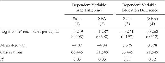
In this section, I examine whether the Great Depression altered the fundamentals of the marriage market. Individuals typically search for mates within a certain age range and within the same race and class. Other large-scale historical events, such as World War I and the Chinese famine have been found to have changed the mating patterns of those affected (Abramitzky, Delavande, and Vasconcelos Reference Delavande and Vasconcelos2011; Almond et al. Reference Almond, Edlund, Li and Zhang2007). Table 4 shows the results of regressions where the dependent variable is age difference between spouses (column (1) and (2)) or education years difference between spouses (columns (3) and (4)). I report estimates for the state (column (1) and (3)) and SEA level (columns (2) and (4)). At the SEA level, lowered local retail sales are associated with a smaller age gap between husband and wife. The estimate implies a 25 percent drop in retail sales would lower the age gap between spouses by 3.8 months. The estimate is only marginally statistically significant though, and no effect is found at the state level. No statistically significant effects are found on the education difference between spouses. I also find no impact on inter-racial marriage or the propensity of natives to marry foreign borns (results not shown). The Great Depression certainly affected marriage rates; however, the results in Table 4 suggest that it did not affect the fundamentals of the marriage market. Whether they married in the depths of the Depression or during the recovery, individuals married similar spouses in terms of observables (age, race, education).
THE EFFECT OF ECONOMIC CONDITIONS ON AGE AND EDUCATION DISPARITIES BETWEEN SPOUSES

∗ = Significant at the 10 percent level.
∗ = Significant at 5 percent level.
∗∗∗ = Significant at 1 percent level.
Notes:
Variable of interest is log income per capita for state level and log retail sales per capita for the SEA level. Standard errors (in parentheses) are clustered at the location and year level. Other controls: age of marriage, education, dummy if in metropolitan area (for state regressions), race, year fixed effects, and location (SEA or state) fixed effects. Sample includes women age 17–27 at marriage.
Source:
Author's calculations.
Low Migration Sample
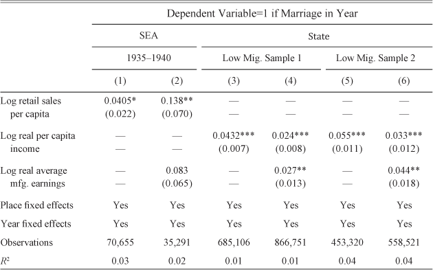
Results using samples where persons are placed with a high degree of accuracy show that migration bias is not driving the observed positive relationship between economic conditions and the probability of marriage. Table 5, columns (1) and (2), shows the results of estimating equation (1) at the SEA level on persons from the 1940 census in the years 1935 and 1939. The individuals in this sample are most likely placed in the correct SEA because SEA data is available from the 1940 census for the years 1935 and 1940 and the economic variables of interest are observed in 1935 and 1939. The estimated coefficients on the variables log manufacturing earnings per capita and log retail sales per capita from this selected sample are less precise due to the smaller sample size, but the coefficients are larger than the coefficients from the corresponding estimations in Table 2 columns (2) and (6). Thus, any bias due to migration is attenuating the estimated coefficients, and the observed positive relationship between the SEA economy and marriage is not caused by selected migration. In columns (3) and (4) of Table 5, I estimate equation (1) at the state level for persons who have at least one match among the four state location variables (current state, birth state, eldest child's birth state, and spouse's birth state). Similar to the results from columns (1) and (2), the coefficients based on this low migration sample are larger than their corresponding coefficients from the estimation based on the entire sample (Table 1, columns (2) and (6)). In columns (5) and (6), I use a sample where persons have at least two matches among the four state location variables, in other words, at least three of the four state location variables are the same. When this sample with less migration bias than the previous sample is used, the point estimates for the coefficients of interest again increase. The results from Table 5 suggest that misallocation of individuals in the data due to migration attenuates the estimates in Tables 1 and 2 and the actual relationship between economic conditions and the probability of marriage is likely stronger than observed.
THE EFFECT OF ECONOMIC CONDITIONS ON MARRIAGE (LOW MIGRATION SAMPLE)

∗ = Significant at the 10 percent level.
∗ = Significant at 5 percent level.
∗∗∗ = Significant at 1 percent level.
Notes:
Standard errors (in parentheses) are clustered by year and place (SEA or state). Other controls: age, age squared, dummy if in metropolitan area, education, race, and census year dummy. Sample includes women age 17–27. Low migration sample 1 is persons who have at least one match among the variables: current state, spouse's birth state, own birth state, and eldest child's birth state. Low migration sample 2 are persons who have at least two matches among the variables: current state, spouse's birth state, own birth state, and eldest child's birth state.
Source:
Author's calculations.
Implications
This subsection uses the results from the previous estimations to understand the extent to which the variation in GDP can explain the marriage patterns over the 1930s. The marriage rate fell by about 12 percent from 1929 to 1932 for women age 14 to 40.Footnote 18 My estimates suggest that GDP accounts for about 75 percent of this downturn. Retail sales fell by 38 percent from 1929 to 1932, an average of $55 per year. If I re-estimate equation (1) with year fixed effects for women age 14 to 40 at the SEA level, I find that an annual retail sales per capita decline of $55 would lower the probability of marriage by an average of 2.6 percent per annum, producing a predicted marriage rate in 1932 of 79.1 marriages per 1,000 unmarried women age 14–40, compared to the actual marriage rate of 76.6 marriages per 1,000 unmarried women age 14–40. The predicted drop represents an 8.7 percent decline, while the actual decline was 11.6 percent. By 1937 the marriage rate had rebounded to its pre-Depression level. My estimates suggest that retail sales per capita can account for about 70 percent of the rebound. No retail sales per capita data exist for 1937, but retail sales per capita grew by an average of $32 per year from 1933 to 1935. I estimate that an annual increase of $32 per year from 1933 to 1937 would increase the marriage rate from 80.7 marriages per 1,000 unmarried women aged 14–40 in 1933 to 87.4 in 1937, an 8 percent increase. The actual increase was 11.8 percent.
LONG-RUN IMPACT OF THE GREAT DEPRESSION ON MARRIAGE
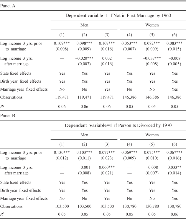
In this section, I examine the impact of the Great Depression on marriage in the subsequent decades. Thus far, I have focused on the effects of the economy on marriage during the 1920s and 1930s. I have provided evidence that the economic downturn negatively impacted marriage rates. However, the data does not suggest that this effect was long lasting, marriage rates quickly recovered, and women who came of age during the downturn were no more likely to never marry than women from other cohorts. The Great Depression did not give rise to a generation of lifelong bachelors and spinsters, but were there other long-term effects of the Great Depression on marriage? The conceptual framework outlined previously indicates that couples that marry during downturns might be better matched on other aspects outside of the income prospects of the male. Another possibility is that courtship during tough economic periods creates strong bonds. In either case, marriages formed in times of economic hardship would be less susceptible to divorce than other marriages.
I test the longevity of marriages formed in the interwar period by examining individuals in 1960 and 1970. The 1960 and 1970 censuses have a much richer set of marriage variables than previous censuses: they list the birth and marriage quarters, age at first marriage, and number of times married.Footnote 19 I limit the sample to individuals whose first marriage occurred between 1921 and 1940. I then examine whether economic conditions at the time of first marriage affected their marriage's longevity by performing the following estimation:

where Dijc is a first marriage failure dummy variable for individual i in state j of the marriage year cohort c. It takes value 1 if the person observed in 1960/70 reports being separated or divorced, or if they currently are in their second or more marriage and their first marriage did not end due to death.Footnote 20 The variable of interest is Incomejc : it is the average log real per capita income in an individual's state for the three years prior to their marriage year. I include birth year fixed effects to account for any difference in divorce across age groups, for example, younger individuals may have less stigma associated with divorce. I also include state fixed effects to account for any differences in the acceptance/prevalence of divorce across states. The vector, xi , contains individual characteristics that may influence the failure of an individual's marriage: race, age at first marriage, and education.
Table 6 shows the effect of state economic conditions prior to an individual's marriage on the survival of that marriage. Panel A shows the results for the 1960 census, while panel B are the 1970 results. Columns (1)–(3) display the effects when the estimation is limited to men and columns (4)–(6) show the results for the women. The estimates suggest that marrying in a prosperous period increases the probability that the marriage will end. For example, the results imply that a man's marriage in 1929 (a year following the relatively affluent period of 1927–1929) was 15 percent more likely to end by 1960 compared to a marriage in 1933, a year following the fallow years of 1931–1933. In columns (2) and (5), I add average real log income per capita for the three years following an individual's marriage. Economic conditions just after marriage do not have a clear effect. The results without marriage year fixed effects suggest couples that experience prosperous years right after marriage are slightly more likely to stay married. In column (3) and (6), I add marriage year fixed effects. Marriage year fixed effects will account for any systematic prevalence of divorce between marriage years. They will also control for any confounding factors from a given marriage year that may be influencing divorce, for instance, if persons married in 1940 were more likely to have served in WWII and that increased the probability of divorce. However, including this fixed effect perhaps leads to over-identification, because much of the variation in economic conditions occurs across marriage years. Furthermore, a portion of the effect of interest is the difference between being married in boom years versus bust years; controlling for marriage year will remove some of the relevant variation in the variable of interest. With these caveats noted, columns (3) and (6) show the results of including marriage year fixed effects in the estimation: The coefficient on real log per capita income prior to marriage does not change significantly; however, the coefficient on income after marriage becomes statistically insignificant with the 1960 sample and positive with the 1970 sample.
LONG-RUN IMPACT OF THE GREAT DEPRESSION ON DIVORCE

∗ = Significant at the 10 percent level.
∗ = Significant at 5 percent level.
∗∗∗ = Significant at 1 percent level.
Notes:
Standard errors (in parentheses) are clustered by marriage year and state. Other controls: age of marriage, veteran status (for males in the 1960 census), education, and race.
Source:
Author's calculations.
CONCLUSION
Economic conditions strongly influenced marriage decisions in the tumultuous 1930s. I find a relationship between economic conditions and marriage at all levels of geographic aggregation: national, state, and SEA. My results imply that the drop in incomes from 1929 to 1932 lowered a woman's probability of marriage by about 6–9 percent. The channel through which local economic conditions affected marriage is the economic viability of males, as I observe statistically significant effects of male manufacturing earnings and male employment on marriage outcomes.
Several scholars have shown that the Great Depression had long-term effects on society and the individuals who lived through it. Great Depression cohorts are more risk averse than average and have a lower taste for material goods (Malmiender and Nagel Reference Malmendier and Nagel2009; Easterlin Reference Easterlin1966). This article posits that another long-term effect of the Great Depression is marriage stability. While the economic crash of the early 1930s certainly reduced marriage rates, the effects were not long lasting. Marriage rates rebounded during the economic recovery: marriage was merely delayed, not denied. The true long-term effect on marriage was longevity. I show that marriages formed in tough economic times were more likely to last than those made in more prosperous times. I theorize that individuals who married during periods of economic uncertainty must have matched well on qualities other than economic viability or the couples forged strong bonds during their courtship during the tumultuous Depression years. When the economy rebounded, these marriages were then well suited to survive and weather further swings in the economy. The Great Depression may have dealt an immediate blow to marriage formation, but in the long run, it engendered more stable, successful unions.