





 where



1 Introduction
Let
 $ (X,d,T,\mu ) $
be a probability measure-preserving system endowed with a compatible metric
 $ d $
so that
 $ (X,d) $
is complete and separable. A corollary of the well-known Poincaré’s recurrence theorem (see e.g. [Reference Furstenberg9, Theorem 3.3]) asserts that
 $ \mu $
-almost all points
 $ x\in X $
are recurrent, that is,
 $$ \begin{align*} \liminf_{n\to\infty}\,d(T^nx,x)=0. \end{align*} $$
This is a qualitative statement in nature. The first quantitative result was given by Boshernitzan [Reference Boshernitzan6].
Theorem 1.1. [Reference Boshernitzan6, Theorem 1.2]
Let
 $ (X,d,T,\mu ) $
be a probability measure-preserving system endowed with a metric
 $ d $
. Assume that for some
 $ \alpha>0 $
, the
 $ \alpha $
-Hausdorff measure
 $ \mathcal H^\alpha $
is
 $ \sigma $
-finite on
 $ (X,d) $
. Then, for
 $ \mu $
-almost every (a.e.)
 $ x\in X $
, we have
 $$ \begin{align*}\liminf_{n\to\infty} n^{1/\alpha}\,d(T^nx,x)<\infty.\end{align*} $$
Moreover, if
 $ \mathcal H^\alpha (X)=0 $
, then for
 $ \mu $
-a.e.
 $ x\in X $
, we have
 $$ \begin{align*}\liminf_{n\to\infty} n^{1/\alpha}\,d(T^nx,x)=0.\end{align*} $$
Further improvements were established by Barreira and Saussol [Reference Barreira and Saussol5] who related the recurrence rate to the local pointwise dimension of
 $\mu $
.
Boshernitzan’s result can be reformulated as follows. For
 $ \mu $
-a.e.
 $ x $
, there is a constant
 $ c(x)>0 $
such that
 $$ \begin{align} d(T^nx,x)<c(x)n^{-1/\alpha}\quad\text{ for infinitely many }n\in\mathbb N \end{align} $$
or, equivalently,

where  denotes the indicator function of the set
 $ E $
, and
 $B(x,r)$
denotes the open ball with center
 $x\in X$
and radius
 $r>0$
. The first reformulation (1.1) leads to understanding the
 $\mu $
-measure of the recurrence set
 $$ \begin{align} \mathcal R(\{r_n\}):=\{x\in X: d(T^nx,x)<r_n\text{ for infinitely many } n\in\mathbb N\}, \end{align} $$
where
 $ \{r_n\} $
is a sequence of non-negative real numbers. For some rapidly mixing dynamical systems (see [Reference Baker and Farmer2, Reference Baker and Koivusalo3, Reference Chang, Wu and Wu7, Reference He and Liao11, Reference Hussain, Li, Simmons and Wang13, Reference Kirsebom, Kunde and Persson15, Reference Kleinbock and Zheng16]), it has been verified that
 $\mu (\mathcal R(\{r_n\})) $
obeys a zero-one law according to the convergence or divergence of the series
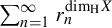 $ \sum _{n=1}^{\infty }r_n^{\text {dim}_{\text {H}} X} $
, where
 $ \text {dim}_{\text {H}} $
stands for the Hausdorff dimension. Such a zero-one law is also referred to as a dynamical Borel–Cantelli lemma for recurrence.
The second reformulation (1.2) leads to further quantification of the divergence rate of the sequence with respect to
 $ n $

It is reasonable to expect that the following stronger statement would hold. If the system mixes sufficiently fast, then

where
 $ c(x) $
is a constant that depends on
 $ x $
. Such results are called the strong dynamical Borel–Cantelli lemma for recurrence. Apparently, if the sum
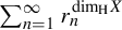 $ \sum _{n=1}^\infty r_n^{\text {dim}_{\text {H}} X} $
diverges and (1.4) holds, then one can deduce that
 $ \mu (\mathcal R(\{r_n\}))=1 $
. In [Reference Persson19], assuming exponential decay of correlations (see Condition I below) together with a condition analogous to Condition II stated later, Persson proved a strong dynamical Borel–Cantelli lemma, similar to (1.4), for a class of dynamical systems on the unit interval. This result was subsequently generalized by Rodriguez Sponheimer [Reference Rodriguez Sponheimer22] to a more general setting including Axiom A diffeomorphisms. Notably, both results require the sequence
 $ \{r_n\} $
to satisfy
 $$ \begin{align} \lim_{a\to 1^+}\limsup_{n\to\infty}\frac{r_n}{r_{an}}=1\quad\text{and}\quad r_{n}\ge \frac{(\log n)^{4+\varepsilon}}{n}\quad\text{ for some } \varepsilon>0. \end{align} $$
Naturally, one would like to prove (1.4) without assuming (1.5), as (1.4) with
 $ x $
replaced by a fixed center
 $ y\in X $
has been verified in various rapidly mixing systems, see [Reference Chernov and Kleinbock8, Reference Kim14, Reference Li, Liao, Velani and Zorin18, Reference Philipp21]. To this end, we need to impose stronger conditions on the underlying dynamical system than those in [Reference Persson19, Reference Rodriguez Sponheimer22].
Let us begin with some notation. Let
 $ X $
be the unit cube
 $ [0,1]^d $
endowed with the maximum norm
 $ |\cdot | $
. The closure, boundary,
 $\varepsilon $
-neighborhood, and cardinal number of
 $ A $
will be denoted by
 $ \overline A $
,
 $ \partial A $
,
 $ A_\varepsilon $
, and
 $ \# A $
, respectively. Let
 $ C^{\theta }([0,1]^d) $
be the space of
 $ \theta $
-Hölder continuous functions endowed with the
 $ \theta $
-Hölder norm
 $$ \begin{align*} \|f\|_{\theta}:=\max_{\mathbf{x}\in[0,1]^d}|f(\mathbf{x})|+ \sup\bigg\{\frac{|f(\mathbf{x})-f(\mathbf{y})|}{|\mathbf{x}-\mathbf{y}|^{\theta}}: \mathbf{x},\mathbf{y}\in[0,1]^d\bigg\}. \end{align*} $$
Let
 $ \{U_i\}_{i\in \mathcal I} $
be a countable family of pairwise disjoint open subsets in
 $ [0,1]^d $
with
 $ \bigcup _{i\in \mathcal I}\overline {U_i}=[0,1]^d $
. The following conditions on the measure-preserving dynamical system
 $ ([0,1]^d,T,\mu ) $
will play a central role in our work.
Condition I. (Exponential decay of correlations) Given
 $ 0<\theta \le 1 $
, there exist constants
 $ \tau =\tau (\theta )>0 $
and
 $ C=C(\theta )>0 $
such that for all
 $ f\in C^\theta ([0,1]^d) $
,
 $ g\in L^1(\mu ) $
, and all
 $ n\ge 0 $
,
 $$ \begin{align} \bigg|\!\int f\cdot g\circ T^n \, {d} \mu-\int f \, {d} \mu\int g \, {d} \mu\bigg|\le Ce^{-\tau n}\|f\|_\theta|g|_1, \end{align} $$
where
 $|g|_1=\int |g| \, {d}\mu $
.
Condition II. The
 $ T $
-invariant measure
 $ \mu $
is absolutely continuous with respect to the d-dimensional Lebesgue measure
 $ \mathcal L^d $
for which the density function
 $ h $
belongs to
 $ L^q(\mathcal L^d) $
for some
 $ q>1 $
.
Condition III. There exists
 $ L>0 $
such that for any
 $ i\ge 1 $
and any
 $ \mathbf {x},\mathbf {y}\in \overline {U_i} $
,
 $$ \begin{align} |T\mathbf{x}-T\mathbf{y}|\ge L|\mathbf{x}-\mathbf{y}|. \end{align} $$
Condition IV. There exist constants
 $ 0<\alpha \le d $
,
 $\varepsilon _0>0$
, and
 $ K_1>0 $
such that
 $$ \begin{align*} \sup_{i\in\mathcal I}\sup_{0<\varepsilon<\varepsilon_0}\frac{\mathcal L^d((\partial U_i)_\varepsilon)}{\varepsilon^\alpha}<K_1. \end{align*} $$
Condition V. There exist a set
 $ \mathcal A\subset [0,1]^d $
, and constants
 $ \beta _1,\beta _2>0 $
and
 $ K_2>0 $
such that for any
 $ 0<r<1 $
,
 $$ \begin{align*}\#\bigg\{i\in \mathcal I:U_i\nsubseteq \bigcup_{x\in \mathcal A} B(x,r)\bigg\}\le K_2r^{-\beta_1}\end{align*} $$
and
 $$ \begin{align*}\mathcal L^d\bigg(\bigcup_{x\in \mathcal A} B(x,r)\bigg)\le K_2r^{\beta_2}.\end{align*} $$
Remark 1.2.
-
(1) Condition I is satisfied by many dynamical systems, such as the Gauss map [Reference Philipp21],
 $\beta $
-transformations [Reference Philipp21], and expanding toral endomorphisms [Reference Baladi4, Theorem 2.3].
-
(2) In [Reference Allen, Baker and Bárány1, Theorem 2.6], Allen, Baker, and Bárány showed that for non-uniform Bernoulli measure on the shift space, the convergence/divergence of the natural volume sum does not always determine the measure of a recurrence set. Consequently, to establish the (strong) dynamical Borel–Cantelli lemma for recurrence, it is essential that
$\mu $
be an absolutely continuous measure with respect to
$\mathcal L^d$
. Additionally, the technical conditions
$h\in L^q(\mathcal L^d)$
with
$q>1$
is needed to effectively estimate the measure of certain sets (see Lemma 2.1). -
(3) Although Condition III does not assume that T is expanding, that is,
$L>1$
, to the author’s best knowledge, systems satisfying Condition I are usually expanding. -
(4) Condition IV says that the boundaries of elements in the partition
$ \{U_i\}_{i\in \mathcal I} $
are sufficiently regular. If
$ \mathcal I $
is finite and the boundary of each
$ U_i $
is included in a
$ C^1 $
piecewise embedded compact submanifold of codimension one, then Condition IV holds with
$ \alpha =1 $
. This condition arises for a natural reason. What needs to be dealt with is the correlations between sets, while Condition I only gives an estimate of the correlations between functions. Therefore, we need to approximate the indicator functions of the sets under consideration with Hölder continuous functions, which leads to Condition IV. -
(5) Condition V says that most elements in
$ \{U_i\}_{i\in \mathcal I} $
will concentrate on a set with small Lebesgue measure. If
$ \mathcal I $
is finite, then we can take
$ \mathcal A=\emptyset $
, and Condition V holds with arbitrary positive
$ \beta _1 $
and
$ \beta _2 $
. For the Gauss map, the associated partition
$ \{U_i\}_{i\in \mathcal I} $
is infinite. We can take
$ \mathcal A=\{0\} $
and Condition V holds with
$ \beta _1=\beta _2=1 $
. -
(6) It is worth pointing out that although Conditions I–V are seemingly restrictive, there are still many dynamical systems that satisfy these conditions, such as the Gauss map,
$\beta $
-transformations, and expanding toral endomorphisms.




For any
 $ \mathbf {x}=(x_1,\ldots ,x_d)\in [0,1]^d $
and
 $ \mathbf {r}=(r_1,\ldots ,r_d)\in (\mathbb R_{\ge 0})^d $
, let
 $$ \begin{align*}R(\mathbf{x},\mathbf{r}):=\prod_{i=1}^{d}(x_i-r_i,x_i+r_i)\end{align*} $$
be a hyperrectangle. Motivated by the weighted theory of Diophantine approximation, for a sequence
 $ \{\mathbf {r}_n\} $
of vectors with
 $ \mathbf {r}_n=(r_{n,1},\ldots ,r_{n,d})\in (\mathbb R_{\ge 0})^d $
, we define
 $$ \begin{align} \mathcal R(\{\mathbf{r}_n\})=\{\mathbf{x}\in [0,1]^d:T^n\mathbf{x}\in R(\mathbf{x},\mathbf{r}_n)\text{ for infinitely many } n\in\mathbb N \}. \end{align} $$
If all the entries of
 $ \mathbf {r}_n $
coincide, that is,
 $ r_{n,1}=\cdots =r_{n,d}=r_n $
, then
 $ \mathcal R(\{\mathbf {r}_n\}) $
is nothing but
 $\mathcal R(\{r_n\}) $
defined in (1.3).
Theorem 1.3. Suppose that the measure-preserving dynamical system
 $ ([0,1]^d,T,\mu ) $
satisfies Conditions I–V. Then,
 $$ \begin{align*} \sum_{n=1}^{\infty} r_{n,1}\cdots r_{n,d}<\infty\quad\Longrightarrow\quad\mu(\mathcal R(\{\mathbf{r}_n\}))=0. \end{align*} $$
Moreover, if
 $\lim _{n\to \infty }|\mathbf {r}_n|=0$
and
 $ \sum _{n=1}^{\infty } r_{n,1}\cdots r_{n,d}=\infty $
, then for
 $ \mu $
-a.e.
 $ \mathbf {x} $
,

where h is the density function given in Condition II.
Remark 1.4. After completing this paper, Levesley et al [Reference Levesley, Li, Simmons and Velani17], Persson and Rodriguez Sponheimer [Reference Persson and Rodriguez Sponheimer20], and Huang, Li, and Velani [Reference Huang, Li and Velani12], derived the asymptotic formula for recurrence under various settings, but without imposing any conditions on the sequence
 $\{r_n\}$
. More precisely, for any
 $\mathbf {x}$
, let
 $r_n(\mathbf {x})$
be defined by the relation
 $\mu (B(\mathbf {x},r_n(\mathbf {x})))=r_n$
. The aforementioned results [Reference Huang, Li and Velani12, Reference Persson and Rodriguez Sponheimer20] show that for
 $\mu $
-a.e.
 $\mathbf {x}$
,

where
 $\Phi (N)=\sum _{n=1}^{N}r_n$
. It is worth emphasizing that, in their framework [Reference Huang, Li and Velani12, Reference Persson and Rodriguez Sponheimer20], the recurrence rate depends not only on the sequence
 $\{r_n\}$
, but also on the initial point
 $\mathbf {x}$
. This dependence on
 $\mathbf {x}$
is essential for obtaining the asymptotic formula (1.10). We remark that (1.10) also holds in the current setting (see Theorem 3.1 and Lemma 3.8). Moreover, compared with the results in [Reference Huang, Li and Velani12, Reference Levesley, Li, Simmons and Velani17, Reference Persson and Rodriguez Sponheimer20], our result remains valid for the
 $\beta $
-transformation with non-integer
 $\beta> 1$
, as well as for expanding toral endomorphisms induced by non-diagonal matrices.
Remark 1.5. The restriction of X to
 $[0,1]^d$
is not necessary. In fact, if X is a compact subset of
 $\mathbb R^d$
with smooth boundaries and
 $(X,T,\mu )$
satisfies Conditions I–V, then we can define a new map
 $\tilde T:[0,1]^d\to [0,1]^d$
as follows. For any
 $\mathbf {x}\in [0,1]^d$
,
 $$ \begin{align*}\tilde T(\mathbf{x})=\begin{cases} \mathbf{x}&\text{if }g(\mathbf{x})\notin X,\\ g^{-1}(T\circ g(\mathbf{x}))&\text{if }g(\mathbf{x})\in X, \end{cases}\end{align*} $$
where
 $D=\max \{|\mathbf {y}|:\mathbf {y}\in X\}$
and
 $g(\mathbf {x})=2D\mathbf {x}-(D,D,\ldots ,D)$
. Theorem 1.3 then applies to
 $([0,1]^d,\tilde T,\tilde T_*\mu )$
and, hence, to
 $(X,T,\mu )$
, where
 $\tilde T_*\mu $
is the pushforward of
 $\mu $
.
Remark 1.6. In [Reference He and Liao11], the author and Liao proved that under conditions similar to Conditions I–V, the
 $ \mu $
-measure of
 $ \mathcal R(\{\mathbf {r}_n\}) $
is either zero or one according as the series
 $ \sum _{n=1}^{\infty }r_{n,1}\cdots r_{n,d} $
converges or not. However, the results in [Reference He and Liao11] are not applicable to the Gauss map, as the authors required the partition
 $ \{U_i\}_{i\in \mathcal I} $
to be finite. Such an assumption is not assumed here and the conclusion is stronger than theirs. Our methods also work under the setting of [Reference He and Liao11], whence the strong dynamical Borel–Cantelli lemma applies to a broad class of expanding matrix transformations, not limited to expanding toral endomorphisms.
Remark 1.7. The proof of Theorem 1.3 partially makes use of the geometric properties of Euclidean space that do not necessarily hold for other metric spaces. For example, any hypercube can be partitioned into smaller hypercubes of equal length and the volume of arbitrary annuli
 $B(\mathbf {x},r+\varepsilon )\setminus B(\mathbf {x},r)$
is bounded by
 $\varepsilon $
up to a multiplicative constant, and so on. The same properties are also implicitly used in [Reference He and Liao11].
1.1 Differences from the shrinking target sets
We take this opportunity to compare our result with those on the shrinking target sets, where the latter, stated in what we are interested in in this paper, aim at establishing the following. For a fixed
 $\mathbf {y}\in [0,1]^d$
,

The main difference is that the center of the shrinking targets
 $R(\mathbf {y},\mathbf {r}_n)$
is independent of the selection of the initial point
 $\mathbf {x}$
. This minor difference did cause some non-trivial difficulties. Note that
 . In view of Theorem 3.1, the key to prove (1.11) is to estimate the correlations
 $$ \begin{align} \mu(T^{-m}R(\mathbf{y},\mathbf{r}_m)\cap T^{-n}R(\mathbf{y},\mathbf{r}_n))\quad\text{for } 0<m<n. \end{align} $$
Using the T-invariance of
 $\mu $
and Lemma 2.3 (a consequence of Condition I), (1.11) follows with some standard calculations (see e.g. [Reference Levesley, Li, Simmons and Velani17, Proof of Proposition 3.5]). However, in the recurrent setting,
 cannot be expressed as the
 $T^n$
-inverse image of some sets, so the invariance of
 $\mu $
and Lemma 2.3 cannot be used directly. Following [Reference Hussain, Li, Simmons and Wang13], one way to overcome this difficulty is to look at the set
 $E_n$
locally by intersecting a small ball B. Then,
 $B\cap E_n$
can be almost written as
 $B\cap T^{-n}R_n$
for some hyperrectangle
 $R_n$
(see Lemma 3.2), and the T-invariance of
 $\mu $
and Lemma 2.3 can be applied. However, in comparison to (1.12), the correlations with which we are going to deal become
 $$ \begin{align*} \mu(B\cap T^{-m}R_m\cap T^{-n}R_n)\quad\text{for some hyperrectangles }R_m \text{ and }R_n \text{ with } 0<m<n. \end{align*} $$
These are 3-fold correlations and Lemma 2.3 does not provide a good estimate for them unless
 $m\ge c\log n$
for some large constant
 $c>0$
(see Lemma 3.5 and Remark 3.6). This is partly why Persson [Reference Persson19] and Rodriguez Sponheimer [Reference Rodriguez Sponheimer22] needed (1.5). Assuming the property of short return times, the condition in (1.5) was subsequently removed in the recent work by Persson and Rodriguez Sponheimer [Reference Persson and Rodriguez Sponheimer20]. Unlike their methods, to avoid assuming the condition in (1.5), we impose two geometric conditions (Conditions IV and V) and adopt some of the ideas from [Reference He and Liao11] by the author and Liao (see Lemma 3.7). However, because the setting is different and our conclusions are stronger, the proofs differ.
2 Correlations of sets with regular boundaries
In this section, we give correlation estimates for sets with regular boundaries. We begin with a simple estimation on measurable subsets which will be frequently referenced in the subsequent discussion.
Throughout, for positive-valued functions f and g, we write
 $f\ll g$
if there exists a constant
 $c>0$
such that
 $f(x)\le cg(x)$
for all x. We write
 $f\asymp g$
if
 $f\ll g\ll f$
.
Lemma 2.1. Let
 $ s=1-1/q $
. For any measurable set
 $ F $
, we have
 $$ \begin{align*}\mu(F)\le |h|_q\mathcal L^d(F)^s,\end{align*} $$
where
 $ |h|_q=(\int |h|^q \, {d}\mathcal L^d)^{1/q} $
is the
 $ L^q $
-norm of
 $ h $
.
Proof. By Hölder’s inequality,

By approximating the indicator function of a set with Lipschitz functions, Condition I enables us to estimate correlations for sets beyond Hölder continuous functions.
Lemma 2.2. Let
 $ E $
and
 $ F $
be two measurable sets. Then, for
 $ 0<\varepsilon <1 $
,
 $$ \begin{align*} \mu(E\cap T^{-n}F)\le \mu(F)(\mu(E)+\mu((\partial E)_\varepsilon)+2Ce^{-\tau n}/\varepsilon) \end{align*} $$
and
 $$ \begin{align*} \mu(E\cap T^{-n}F)\ge \mu(F)(\mu(E)-\mu((\partial E)_\varepsilon)-Ce^{-\tau n}/\varepsilon). \end{align*} $$
Proof. Let
 $ 0<\varepsilon <1 $
. Define
 $$ \begin{align*}f_\varepsilon(x)=\begin{cases}\displaystyle 1-\frac{d(x,E)}{\varepsilon}&\text{if } d(x,E)<\varepsilon ,\\ 0&\text{if } d(x,E)\ge \varepsilon. \end{cases}\end{align*} $$
It is not difficult to verify that
 $ f_\varepsilon $
is Lipschitz with Lipschitz constant
 $ 1/\varepsilon $
. Hence,
 $ f_\varepsilon \in C^\theta ([0,1]^d) $
. Applying the exponential decay of correlations (see Condition I) to
 $ f=f_\varepsilon $
and
 , we have

Note that
 $ f_\varepsilon (x)=1 $
for
 $ x\in E $
and the support of
 $ f_\varepsilon $
is contained in
 $ E_\varepsilon = E\cup (\partial E)_\varepsilon $
. Thus, we have
 $$ \begin{align*}\int f_\varepsilon \, {d}\mu\le \mu(E_\varepsilon)\le \mu(E)+\mu((\partial E)_\varepsilon)\end{align*} $$
and so

To prove the other inequality, by letting
 $ E_{-\varepsilon }=E\setminus (\partial E)_\varepsilon $
, we see that
 $$ \begin{align*}x\in E_{-\varepsilon}\quad\Longrightarrow\quad B(x,\varepsilon)\subset E. \end{align*} $$
Define
 $$ \begin{align*}g_\varepsilon(x)=\begin{cases}\displaystyle 1-\frac{d(x,E_{-\varepsilon})}{\varepsilon}&\text{if } d(x,E_{-\varepsilon})<\varepsilon,\\ 0&\text{if } d(x,E_{-\varepsilon})\ge \varepsilon. \end{cases}\end{align*} $$
Clearly, by definition,

Now, employing the argument similar to above, we arrive at the second inequality of the lemma.
The above lemma suggests that estimating the correlation of some sets requires that the boundaries of these sets are regular enough, which is why we require Condition IV. As a consequence, we get the exponential decay of correlations for hyperrectangles.
Lemma 2.3. Let
 $ R $
be a hyperrectangle and let
 $ F $
be a measurable set. Then, we have
 $$ \begin{align*}|\mu(R\cap T^{-n}F)-\mu(R)\mu(F)|\le c_1\mu(F)e^{-\tau_1n},\end{align*} $$
where
 $ c_1=4d|h|_q+2C $
and
 $ \tau _1=s\tau /(1+s) $
.
Proof. Note that for any
 $ \varepsilon>0 $
,
 $ (\partial R)_\varepsilon $
is contained in
 $ 2d $
hyperrectangles, each of which has volume less than
 $ 2\varepsilon $
. By Lemma 2.1,
 $$ \begin{align*} \mu((\partial R)_\varepsilon)\le |h|_q\mathcal L^d((\partial R)_\varepsilon)^s\le 4d|h|_q\varepsilon^s. \end{align*} $$
Applying Lemma 2.2 with
 $ \varepsilon =e^{-\tau n/(1+s)} $
, we have
 $$ \begin{align*}\mu(R\cap T^{-n}F)\le \mu(F)(\mu(R)+4d|h|_qe^{-s\tau n/(1+s)}+2Ce^{-s\tau n/(1+s)})\end{align*} $$
and
 $$ \begin{align*}\mu(R\cap T^{-n}F)\ge \mu(F)(\mu(R)-4d|h|_qe^{-s\tau n/(1+s)}-Ce^{-s\tau n/(1+s)}),\end{align*} $$
which finishes the proof.
The proof of the divergence part of Theorem 1.3 crucially relies on the following two technical lemmas. The ideas originate from [Reference He and Liao11, Lemmas 2.8 and 2.10], but the proofs are different because, in the current setting,
 $ T $
is not necessarily expanding and the partition
 $ \{U_i\}_{i\in \mathcal I} $
may be infinite. For any
 $n\ge 1$
, define
 $$ \begin{align*}\mathcal F_n:=\{U_{i_0}\cap\cdots\cap T^{-(n-1)}U_{i_{n-1}}:i_0,\ldots,i_{n-1}\in\mathcal I\}.\end{align*} $$
Lemma 2.4. There exists a constant
 $ c_2 $
such that for any
 $0<\varepsilon <\varepsilon _0$
with
 $\varepsilon _0$
given in Condition IV, any hyperrectangles
 $ R_1,R_2\subset [0,1]^d $
, and any
 $J_n\in \mathcal F_n$
,
 $$ \begin{align*} \mu((\partial(J_n\cap R_1\cap T^{-n}R_2))_\varepsilon)\le c_2(\max(n, L^{-nd})\varepsilon^{\min(1,\alpha)})^{s}. \end{align*} $$
Proof. Let
 $0<\varepsilon <\varepsilon _0$
. First, we claim that for any
 $ J_n\in \mathcal F_n $
,
 $$ \begin{align} \mathcal L^d((\partial J_n)_\varepsilon)\ll \begin{cases} \dfrac{L^{-nd}-1}{L^{-d}-1}\varepsilon^\alpha&\text{if }L<1,\\ n\varepsilon^\alpha&\text{if }L\ge 1, \end{cases} \end{align} $$
where
 $0<\alpha \le d$
is given in Condition IV. We proceed by induction. For
 $ n=1 $
, we have
 $\partial J_1=\partial U_i$
for some
 $i\in \mathcal I$
, and so this is implied by Condition IV.
Assume that (2.1) holds for some
 $ n\ge 1 $
. We will prove that (2.1) holds for
 $ n+1 $
. Write
 $ J_{n+1}=J_{n}\cap T^{-n}(U_{i_n}) $
, where
 $ J_n\in \mathcal F_n $
and
 $ i_n\in \mathcal I $
. By Condition III, the inverse of the map
 $ T^n|_{J_{n}}\colon J_n\to T^nJ_n $
, denoted by
 $ f_n $
, exists and satisfies
 $$ \begin{align} |f_n(\mathbf{x})-f_n(\mathbf{y})|\le L^{-n}|\mathbf{x}-\mathbf{y}| \quad\text{for any } \mathbf{x},\mathbf{y}\in T^nJ_n. \end{align} $$
Since
 $ f_n $
is invertible and Lipschitz, we have
 $$ \begin{align} \partial J_{n+1}&=\partial (J_{n}\cap T^{-n}(U_{i_n}))=\partial (f_n(T^nJ_{n}\cap U_{i_n}))\nonumber\\ &=f_n(\partial(T^nJ_{n}\cap U_{i_n})). \end{align} $$
Clearly,
 $ \partial (T^nJ_{n}\cap U_{i_n})\subset \partial (T^nJ_n)\cup \partial U_{i_n} $
. Thus, we get
 $$ \begin{align*}\begin{aligned} \partial J_{n+1}\subset f_n(\partial(T^nJ_n))\cup f_n(\partial U_{i_n})=\partial J_n\cup f_n(\partial U_{i_n}). \end{aligned}\end{align*} $$
Let
 $ \mathcal E $
be a maximal
 $ \varepsilon $
-separated subset of
 $ \partial U_{i_n} $
. The maximal property implies that the balls with radius
 $ \varepsilon /2 $
and center in
 $ \mathcal E $
are pairwise disjoint. Hence, by Condition IV, we have
 $$ \begin{align*} \#\mathcal E\cdot \varepsilon^d\asymp \mathcal L^d((\partial U_{i_n})_{\varepsilon})\ll \varepsilon^\alpha, \end{align*} $$
which implies that
 $$ \begin{align*}\#\mathcal E\ll\varepsilon^{\alpha-d}.\end{align*} $$
Given that
 $ f_n $
is Lipschitz with Lipschitz constant
 $ L^{-n} $
, the image of
 $\mathcal E$
under
 $f_n$
is an
 $ L^{-n}\varepsilon $
-net of
 $ f_n(\partial U_{i_n}) $
. If
 $L<1$
, then we have
 $L^{-n}>1$
, and so
 $ (f_n(\partial U_{i_n}))_\varepsilon $
is contained in the union of balls with radius
 $ 2L^{-n}\varepsilon $
and centers in
 $f_n\mathcal E$
. Thus,
 $$ \begin{align} \mathcal L^d((f_n(\partial U_{i_n}))_\varepsilon)\ll \#f_n\mathcal E\cdot (L^{-n}\varepsilon)^d\le \#\mathcal E\cdot (L^{-n}\varepsilon)^d\ll L^{-nd}\varepsilon^\alpha. \end{align} $$
On the other hand, if
 $L\ge 1$
, then
 $L^{-n}<1$
and so
 $f_n\mathcal E$
is also an
 $\varepsilon $
-net of
 $f_n(\partial U_{i_n})$
. Thus,
 $$ \begin{align*} \mathcal L^d((f_n(\partial U_{i_n}))_\varepsilon)\ll \#f_n\mathcal E\cdot \varepsilon^d\le \#\mathcal E\cdot \varepsilon^d\ll \varepsilon^\alpha. \end{align*} $$
In what follows, we may assume that
 $L<1$
as the argument for
 $L\ge 1$
is similar. Using the inductive hypothesis and (2.4), we have
 $$ \begin{align} \mathcal L^d((\partial J_{n+1})_\varepsilon) &\le \mathcal L^d((\partial J_n)_\varepsilon)+\mathcal L^d((f_n(\partial U_{i_n}))_\varepsilon)\nonumber\\ &\ll\frac{L^{-nd}-1}{L^{-d}-1}\varepsilon^\alpha+L^{-nd}\varepsilon^\alpha\nonumber\\ &=\frac{L^{-(n+1)d}-1}{L^{-d}-1}\varepsilon^\alpha, \end{align} $$
which proves the claim.
Note that
 $\mathcal L^d((\partial R)_\varepsilon )\ll \varepsilon $
. By the same reason as (2.4), we may take
 $ \alpha =1 $
and deduce that
 $$ \begin{align*} \mathcal L^d((f_{n}(\partial R_2))_\varepsilon)\ll L^{-nd}\varepsilon. \end{align*} $$
Similarly, following the same lines as (2.5) with
 $U_{i_n}$
replaced by
 $R_2$
, we have
 $$ \begin{align*}\begin{aligned} \mathcal L^d((\partial (J_n\cap R_1\cap T^{-n}R_2))_\varepsilon)&\le \mathcal L^d((\partial R_1)_\varepsilon)+\mathcal L^d((\partial (J_n\cap T^{-n} R_2))_\varepsilon)\\ &\le \mathcal L^d((\partial R_1)_\varepsilon)+\mathcal L^d((\partial J_n)_\varepsilon)+\mathcal L^d((f_n(\partial R_2))_\varepsilon)\\ &\ll\varepsilon+\frac{L^{-nd}-1}{L^{-d}-1}\varepsilon^\alpha+L^{-nd}\varepsilon\\ &\ll L^{-nd}\varepsilon^{\min(1,\alpha)}. \end{aligned}\end{align*} $$
Apply Lemma 2.1 and the proof is finished.
We will use Condition IV and the last lemma to prove estimations similar to those in [Reference He and Liao11, Lemma 2.10]. However, their methods cannot be directly applied here since the partition
 $ \{U_i\}_{i\in \mathcal I} $
may be infinite. For
 $m<n$
, let
 $$ \begin{align*} D(m,n):=\bigcup_{i=0}^{m-1} \bigg(T^{-i}\bigcup_{x\in \mathcal A}B(x,n^{-7/(s\beta_2)})\bigg) \end{align*} $$
and
 $$ \begin{align*} \begin{aligned} \mathcal F_m(n):=\bigg\{U_{i_0}\cap\cdots\cap T^{-(m-1)}U_{i_{m-1}}:U_{i_j}\nsubseteq \bigcup_{x\in \mathcal A}B(x,n^{-7/(s\beta_2)}), 0\le j\le m-1\bigg\}. \end{aligned} \end{align*} $$
It can be checked that
 $$ \begin{align*}[0,1]^d\setminus D(m,n)\subset \bigcup_{J_m\in\mathcal F_m(n)}\overline{J_m}.\end{align*} $$
In other words,
 $D(m,n)$
denotes the set of points whose forward orbits, under the iteration of T up to
 $m-1$
, hit the set
 $\bigcup _{x\in \mathcal A}B(x,n^{-7/(s\beta _2)})$
at least once. Meanwhile, the set
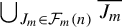 $\bigcup _{J_m\in \mathcal F_m(n)}\overline {J_m}$
is slightly larger than the complement of
 $D(m,n)$
for technical reasons. Additionally, by Condition V, we have
 $$ \begin{align*}\#\mathcal F_m(n)\le (K_2 n^{7\beta_1/(s\beta_2)})^m.\end{align*} $$
Lemma 2.5. There exist constants
 $ c_3 $
and
 $ 0<\eta <\tau _1 $
such that:
-
(1) for any
$m<n$
, we have
$ \mu (D(m,n))\le c_3n^{-6} $
; -
(2) for any
$ m<\sqrt n $
and any hyperrectangles
$ R_1,R_2, R_3\subset [0,1]^d $
, we have
$$ \begin{align*} \sum_{J_m\in\mathcal F_m(n)}\mu(J_m\cap R_1\cap T^{-m}R_2\cap T^{-n}R_3)\le (\mu(R_1\cap T^{-m}R_2)+ c_3e^{-\eta n})\mu(R_3).\end{align*} $$




Proof. (1) By Lemma 2.1 and Condition V,
 $$ \begin{align*} \mu(D(m,n))&\le m\mu\bigg(\bigcup_{x\in \mathcal A}B(x,n^{-7/(s\beta_2)})\bigg)\ll m\mathcal L^d\bigg(\bigcup_{x\in \mathcal A}B(x,n^{-7/(s\beta_2)})\bigg)^s\\ &\ll m\cdot n^{-7}\le n^{-6}. \end{align*} $$
(2) Write
 $L_m=\max (m,L^{-dm})$
and
 $\kappa =\min (1,\alpha )$
. Applying Lemmas 2.2 and 2.4 with
 $ \varepsilon =e^{-\tau n/2} $
, we have
 $$ \begin{align} &\sum_{J_m\in\mathcal F_m(n)}\mu(J_m\cap R_1\cap T^{-m}R_2\cap T^{-n}R_3)\nonumber\\ & \qquad\le \sum_{J_m\in\mathcal F_m(n)}(\mu(J_m\cap R_1\cap T^{-m}R_2)+c_2(L_me^{-\kappa\tau n/2})^s+c_1e^{-\tau n/2})\mu(R_3)\nonumber\\ & \qquad\le (\mu(R_1\cap T^{-m}R_2)+ \# \mathcal F_m(n)(c_2(L_me^{-\kappa\tau n/2})^s+c_1e^{-\tau n/2}))\mu(R_3). \end{align} $$
Since
 $ m\le \sqrt n $
, both terms
 $$ \begin{align*} \# \mathcal F_m(n)\le (K_2 n^{7\beta_1/(s\beta_2)})^m\le e^{\sqrt n\log K_2+7\beta_1\sqrt n\log n/(s\beta_2)}\end{align*} $$
and
 $$ \begin{align*}L_m=\max(m,L^{-dm})\le\max(\sqrt n, e^{-d\sqrt{n}\log L})\end{align*} $$
grow at most subexponentially. Thus, there exist
 $ c_3>0 $
and
 $ 0<\eta <\tau _1 $
such that (2.6) is bounded by
 $$ \begin{align*} (\mu(R_1\cap T^{-m}R_2)+ c_3e^{-\eta n})\mu(R_3). \\[-35pt] \end{align*} $$
3 Proof of Theorem 1.3
This section is dedicated to the proof of Theorem 1.3. To begin, assume that
 $ \sum _{n=1}^{\infty }r_{n,1}\cdots r_{n,d}<\infty $
. In [Reference He and Liao11, Proposition 2.1], the author and Liao established that
 $ \mu (\mathcal R(\{\mathbf {r}_n\}))=0 $
under Condition II and the following exponential decay of correlations for hyperrectangles
 $ R_1 $
and
 $ R_2 $
,
 $$ \begin{align*}|\mu(R_1\cap T^{-n}R_2)-\mu(R_1)\mu(R_2)|\le \mu(R_2)c_1e^{-\tau_1n}.\end{align*} $$
Such a property is also assumed in the present setting (see Condition I and Lemma 2.3), so we can employ the same argument as in [Reference He and Liao11, Proposition 2.1] to conclude the convergence part of the theorem.
Now, suppose that
 $$ \begin{align} \sum_{n=1}^{\infty}r_{n,1}\cdots r_{n,d}=\infty. \end{align} $$
In what follows, to simplify the notation, write
 $$ \begin{align} \gamma_n=r_{n,1}\cdots r_{n,d}. \end{align} $$
Without loss of generality, we further assume that for all
 $ n\in \mathbb N $
,
 $$ \begin{align} \text{either }\quad \gamma_n=0 \quad \text{ or }\quad \gamma_n\ge n^{-2}. \end{align} $$
We will prove the divergence part of the theorem under these assumptions. Indeed, let
 $$ \begin{align*}D=\{n\in\mathbb N: \gamma_n> n^{-2}\} \quad\text{and}\quad D_n=\{1,\ldots, n\}\cap D. \end{align*} $$
Then, by (3.1) and the fact that
 $ \sum _{n=1}^\infty n^{-2}<\infty $
, we have
 $$ \begin{align*} \lim_{N\to\infty}\dfrac{\sum_{n\in D_N}\gamma_n}{\sum_{n=1}^N\gamma_n}=1. \end{align*} $$
On the other hand, since
 $$ \begin{align*}\sum_{n\in\mathbb N\setminus D}\gamma_n\le \sum_{n\in\mathbb N\setminus D}n^{-2}<\infty,\end{align*} $$
the convergence part of Theorem 1.3 implies that for
 $\mu $
-a.e.
 $ \mathbf {x} $
,

For any such
 $ \mathbf {x} $
, it follows that

Then, the divergence part of Theorem 1.3 holds provided that (3.4) holds for
 $ \mu $
-a.e.
 $ \mathbf {x} $
.
Given that the density h of
 $\mu $
may be unbounded, it is more appropriate to study the following auxiliary sets inspired by [Reference Kirsebom, Kunde and Persson15]. For any
 $ \mathbf {x}\in [0,1]^d $
and
 $ n\in \mathbb N $
, let
 $ l_n(\mathbf {x})\in \mathbb R_{\ge 0} $
be the non-negative number such that
 $ \mu (R(\mathbf {x},l_n(\mathbf {x})\mathbf {r}_n))=\gamma _n $
. This is possible, since
 $\mu $
is non-singular. Let
 $$ \begin{align*}\xi_n(\mathbf{x}):=l_n(\mathbf{x})\mathbf{r}_n\in(\mathbb R_{\ge 0})^d.\end{align*} $$
Then,
 $ R(\mathbf {x}, \xi _n(\mathbf {x})) $
is a hyperrectangle obtained by scaling
 $ R(\mathbf {x}, \mathbf {r}_n) $
by a factor of
 $ l_n(\mathbf {x}) $
. Define
 $$ \begin{align*}\hat E_n:=\{\mathbf{x}\in[0,1]^d:T^n\mathbf{x}\in R(\mathbf{x}, \xi_n(\mathbf{x}))\}.\end{align*} $$
The key ingredient for the proof of the divergence case is to use the following quantitative form of the divergence part of the Borel–Cantelli lemma.
Theorem 3.1. [Reference Sprindžuk23, Ch. I, Lemma 10]
Let
 $ \{A_n\} $
be a sequence of measurable sets in a probability space
 $ (X,\nu ) $
. Denote by
 $ A(N,x) $
the number of integers
 $ n\le N $
such that
 $ {x\in A_n} $
. Put
 $$ \begin{align*}\phi(N)=\sum_{n=1}^N\nu(A_n).\end{align*} $$
Suppose that there exists a constant
 $ c $
such that for any
 $ 1\le M<N $
,
 $$ \begin{align*} \sum_{M\le m<n\le N}(\nu(A_{n}\cap A_m)-\nu (A_n)\nu(A_m))\le \sum_{n=M}^Nc\nu(A_n). \end{align*} $$
Then, for any
 $ \varepsilon>0 $
, one has
 $$ \begin{align*} A(N,x)=\phi(N)+O_\varepsilon(\phi^{1/2}(N)\log^{3/2+\varepsilon}\phi(N)) \end{align*} $$
for
 $ \nu $
-a.e.
 $ x $
; in particular, if
 $ \sum _{n=1}^\infty \nu (A_n)=\infty $
, then for
 $\nu $
-a.e. x,
 $$ \begin{align*}\lim_{N\to\infty}\frac{A(N,x)}{\phi(N)}=1.\end{align*} $$
To apply Theorem 3.1, it is essential to estimate both the measure of each
 $ \hat E_n $
and the correlations among the sets
 $ \{\hat E_n\} $
. These aspects will be addressed in the upcoming two subsections, respectively.
3.1 Estimate of the measure of
$\hat {E}_n$

By (3.3), we may assume that
 $ \gamma _n\ge n^{-2} $
. For otherwise by (3.3), we would have
 $ \gamma _n=0 $
and so
 $ \mu (\hat E_n)=0 $
. The following two lemmas coming from [Reference He and Liao11] are useful in estimating the
 $\mu $
-measure of
 $ \hat E_n $
. The first one describes some local structures of
 $ \hat E_n $
; the other one calculates the
 $\mu $
-measure of hyperrectangles related to
 $ \hat E_n $
.
Lemma 3.2. [Reference He and Liao11, Lemma 2.4]
Let
 $ B(\mathbf {x},r) $
be a ball with center
 $ \mathbf {x} $
and
 $ r>0 $
. Then, for any
 $ n\in \mathbb N $
with
 $ \gamma _n\ne 0 $
and any
 $ F\subset B(\mathbf {x},r) $
, we have
 $$ \begin{align*}F\cap T^{-n}R(\mathbf{x},\xi_n(\mathbf{x})-2rn^{2}\mathbf{r}_n)\subset F\cap\hat E_n\subset F\cap T^{-n} R(\mathbf{x},\xi_n(\mathbf{x})+2rn^2\mathbf{r}_n).\end{align*} $$
Lemma 3.3. [Reference He and Liao11, Lemma 2.5]
For any
 $ \mathbf {r}\in (\mathbb R_{\ge 0})^d $
, we have
 $$ \begin{align*} \mu(R(\mathbf{x},\xi_n(\mathbf{x})+\mathbf{r}))&\le \gamma_n+2d|h|_q|\mathbf{r}|^s,\\ \mu(R(\mathbf{x},\xi_n(\mathbf{x})-\mathbf{r}))&\ge \gamma_n-2d|h|_q|\mathbf{r}|^s. \end{align*} $$
Since
 $0<\eta <\tau _1<\tau $
, here and hereafter, we will replace
 $ \tau $
and
 $ \tau _1 $
in Lemmas 2.3 and 2.4 with
 $ \eta $
, and the estimates will still hold. Recall that a ball here is with respect to the maximum norm and thus corresponds to a Euclidean hypercube. The geometry of
 $ [0,1]^d $
allows us to write it as the union of
 $ n^{2d+4d/s} $
pairwise disjoint balls with common radius
 $ n^{-2-4/s} $
. The collection of these balls is denoted by
 $$ \begin{align} \mathcal B_n:=\{B(\mathbf{x}_i,n^{-2-4/s}):1\le i\le n^{2d+4d/s}\}. \end{align} $$
Since
 $ n^{2+4/s} $
is, in general, not an integer, we should use
 $ r=1/[n^{2+4/s}] $
instead of
 $ n^{-2-4/s} $
in the definition of
 $\mathcal B_n$
so that
 $[0,1]^d$
can be partitioned into
 $1/r$
balls of radius r, where
 $ [\cdot ] $
denotes the integer part of a real number. However, to improve the readability, we let the correct definition be implicitly understood throughout the proof. The outcome is invariant under this abuse of notation.
Now, we estimate the
 $\mu $
-measure of
 $ \hat E_n $
.
Lemma 3.4. There exists a constant
 $ c_4 $
such that
 $$ \begin{align*}(1-c_4n^{-2})\gamma_n\le\mu(\hat E_n)\le(1+c_4n^{-2})\gamma_n.\end{align*} $$
Proof. For each ball
 $ B_{n,i}=B(\mathbf {x}_i,n^{-2-4/s})\in \mathcal B_n $
, by Lemma 3.2, we have
 $$ \begin{align*}B_{n,i}\cap\hat E_n\supset B_{n,i}\cap T^{-n}R(\mathbf{x}_i,\xi_n(\mathbf{x}_i)-2n^{-2-4/s}n^2\mathbf{r}_n).\end{align*} $$
Hence,
 $$ \begin{align} \hat E_n\supset \bigcup_{B_{n,i}\in\mathcal B_n}B_{n,i}\cap T^{-n}R(\mathbf{x}_i,\xi_n(\mathbf{x}_i)-2n^{-4/s}\mathbf{r}_n). \end{align} $$
Applying Lemmas 2.3 and 3.3, we have
 $$ \begin{align*} &\mu(B_{n,i}\cap T^{-n}R(\mathbf{x}_i,\xi_n(\mathbf{x}_i)-2n^{-4/s}\mathbf{r}_n))\nonumber\\ &\quad \ge (\mu(B_{n,i})-c_1e^{-\eta n})\mu(R(\mathbf{x}_i,\xi_n(\mathbf{x}_i)-2n^{-4/s}\mathbf{r}_n))\\ &\quad \ge (\mu(B_{n,i})-c_1e^{-\eta n})(\gamma_n-4d|h|_qn^{-4}). \end{align*} $$
Summing over all
 $B_{n,i}\in \mathcal B_{n} $
, we deduce that the
 $ \mu $
-measure of
 $ \hat E_n $
is at least
 $$ \begin{align*}(1-n^{2d+4d/s}\cdot c_1e^{-\eta n})(\gamma_n-4d|h|_qn^{-4}).\end{align*} $$
Since
 $$ \begin{align*} n^{2d+4d/s}e^{-\eta n}\ll n^{-2}\quad\text{and}\quad n^{-4}\le n^{-2}\gamma_n, \end{align*} $$
we conclude that there exists a constant
 $ c_4 $
such that
 $$ \begin{align*}\mu(\hat E_n)\ge (1-c_4n^{-2})\gamma_n.\end{align*} $$
The upper estimation for
 $ \mu (\hat E_n) $
can be proved by replacing (3.6) with
 $$ \begin{align*} \hat E_n\subset \bigcup_{B_{n,i}\in\mathcal B_n}B_{n,i}\cap T^{-n}R(\mathbf{x}_i,\xi_n(\mathbf{x}_i)+2n^{-4/s}\mathbf{r}_n). \\[-48pt] \end{align*} $$
3.2 Estimates for correlations between
$\hat{E}_m $
and
$ \hat{E}_n $
(
$ m < n$
)


Lemma 3.5. There exists a constant
 $ c_5 $
such that for any integers
 $ m $
and
 $ n $
with
 $ \sqrt n\le m<n $
, we have
 $$ \begin{align*} \mu(\hat E_m\cap\hat E_n)\le (1+c_5n^{-2})\gamma_m\gamma_n+c_5e^{-\eta(n-m)}\gamma_n. \end{align*} $$
Proof. Since
 $ m<n $
, we have
 $$ \begin{align*}n^{-2-4/s}m^2\le n^{-2-4/s}n^2= n^{-4/s}.\end{align*} $$
For each ball
 $ B_{n,i}=B(\mathbf {x}_i,n^{-2-4/s})\in \mathcal B_n $
, by Lemma 3.2, we have
 $$ \begin{align} &B_{n,i}\cap \hat E_m\cap \hat E_n\nonumber\\ &\quad \subset B_{n,i}\cap T^{-m}R(\mathbf{x}_i,\xi_m(\mathbf{x}_i)+2n^{-4/s}\mathbf{r}_m)\cap T^{-n}R(\mathbf{x}_i,\xi_n(\mathbf{x}_i)+2n^{-4/s}\mathbf{r}_n) \end{align} $$
and so
 $$ \begin{align*} \begin{aligned} &\hat E_m\cap\hat E_n\\ &\quad \subset \bigcup_{B_{n,i}}B_{n,i}\cap T^{-m}R(\mathbf{x}_i,\xi_m(\mathbf{x}_i)+2n^{-4/s}\mathbf{r}_m)\cap T^{-n}R(\mathbf{x}_i,\xi_n(\mathbf{x}_i)+2n^{-4/s}\mathbf{r}_n). \end{aligned} \end{align*} $$
Applying Lemma 2.3 twice to the sets in (3.7), we have
 $$ \begin{align*} \mu&(B_{n,i}\cap T^{-m}R(\mathbf{x}_i,\xi_m(\mathbf{x}_i)+2n^{-4/s}\mathbf{r}_m)\cap T^{-n}R(\mathbf{x}_i,\xi_n(\mathbf{x}_i)+2n^{-4/s}\mathbf{r}_n))\\ & \le(\mu(B_{n,i})+c_1e^{-\eta m})\mu(R(\mathbf{x}_i,\xi_m(\mathbf{x}_i)+2n^{-4/s}\mathbf{r}_m)\cap T^{-(n-m)}R(\mathbf{x}_i,\xi_n(\mathbf{x}_i)+2n^{-4/s}\mathbf{r}_n))\\ &\le (\mu(B_{n,i})+c_1e^{-\eta m})(\mu(R(\mathbf{x}_i,\xi_m(\mathbf{x}_i)+2n^{-4/s}\mathbf{r}_m))+c_1e^{-\eta(n-m)})\\ &\quad\ \cdot \mu(R(\mathbf{x}_i,\xi_n(\mathbf{x}_i)+2n^{-4/s}\mathbf{r}_n)). \end{align*} $$
By Lemma 3.3, the last quantity is majorized by
 $$ \begin{align*} (\mu(B_{n,i})+c_1e^{-\eta m}) (\gamma_m+4d|h|_qn^{-4}+c_1e^{-\eta(n-m)})(\gamma_n+4d|h|_qn^{-4}).\end{align*} $$
Summing over
 $ B_{n,i}\in \mathcal B_n $
, we have
 $$ \begin{align*}\begin{aligned} \mu(&\hat E_m\cap \hat E_n)\\ & \le (1+c_1n^{2d+4d/s}e^{-\eta m})(\gamma_m+4d|h|_qn^{-4}+c_1e^{-\eta(n-m)})(\gamma_n+4d|h|_qn^{-4}). \end{aligned}\end{align*} $$
From the conditions
 $ \gamma _m\ge m^{-2} $
,
 $ \gamma _n\ge n^{-2} $
and
 $ \sqrt n\le m<n $
, it follows that
 $$ \begin{align*}4d|h|_qn^{-4}\le cn^{-2}\max (\gamma_m,\gamma_n)\quad\mathrm{ and} \quad c_1n^{2d+4d/s}e^{-\eta m}\le c n^{-2}\end{align*} $$
for some absolute constant
 $ c>0 $
. Thus, we have
 $$ \begin{align*}\begin{aligned} &\mu(\hat E_m\cap \hat E_n)\\ &\quad\le (1+cn^{-2})(\gamma_m+cn^{-2}\gamma_m+c_1e^{-\eta(n-m)})\cdot (\gamma_n+cn^{-2}\gamma_n)\\ &\quad = (1+cn^{-2})^3\gamma_m \gamma_n+(1+cn^{-2})^2c_1e^{-\eta (n-m)}\gamma_n. \end{aligned}\end{align*} $$
By choosing a proper constant
 $c_5$
, we arrive at the conclusion.
Remark 3.6. Indeed, with some effort, one can actually show that Lemma 3.5 holds if
 $m\ge c\log n$
for some large constant
 $c>0$
. However, we will not pursue this since
 $m\ge \sqrt n$
is sufficient for us.
The correlation estimates presented in Lemma 3.5 work effectively for the case
 $ {m\ge \sqrt {n}} $
, and the proof relies solely on Conditions I and II. We will employ Lemma 2.5 to estimate the correlations of
 $ \hat E_m\cap \hat {E}_n $
for
 $ m<\sqrt n $
.
Lemma 3.7. There exists a constant
 $ c_6 $
such that for any integers
 $ m $
and
 $ n $
with
 $ {0<m<\sqrt n }$
, we have
 $$ \begin{align*}\mu(\hat E_m\cap \hat E_n)\le(1+c_6m^{-2}) \gamma_m\gamma_n.\end{align*} $$
Proof. Recall the definitions of
 $D(m,n)$
and
 $\mathcal F_m(n)$
in Lemma 2.5. Since
 $D(m,n)\cup \mathcal \bigcup _{J_m\in \mathcal F_m(n)}\overline {J_m}=[0,1]^d$
, by Lemma 2.5,
 $$ \begin{align} \mu(\hat E_m\cap \hat E_n)&\le \mu(D(m,n)\cap\hat E_m\cap \hat E_n)+\sum_{J_m\in\mathcal F_m(n)}\mu(\overline{J_m}\cap \hat E_m\cap \hat E_n)\nonumber\\ &\le c_3n^{-6}+\sum_{J_m\in\mathcal F_m(n)}\mu(J_m\cap \hat E_m\cap \hat E_n)\nonumber\\ &\le c_3n^{-2}\gamma_m\gamma_n+\sum_{J_m\in\mathcal F_m(n)}\mu(J_m\cap \hat E_m\cap \hat E_n), \end{align} $$
where we use
 $\mu (\partial J_m)\asymp \mathcal L^d(\partial J_m)^s=0$
in the second inequality.
Now, we estimate the summation in (3.8). By decreasing the radius of balls in
 $ \mathcal B_n $
by a factor between
 $ 1/2 $
and
 $ 1 $
, we can assume that each ball in
 $ \mathcal B_n $
is contained in a unique ball in
 $ \mathcal B_m $
. This manipulation does not affect the subsequent conclusion. By Lemma 3.2, we have
 $$ \begin{align*}\begin{aligned} &B_{m,j}\cap\hat E_m\cap\hat E_n=\bigcup_{B_{n,i}:B_{n,i}\subset B_{m,j}}(B_{m,j}\cap\hat E_m)\cap (B_{n,i}\cap\hat E_n)\\ &\quad\subset \bigcup_{B_{n,i}:B_{n,i}\subset B_{m,j}} B_{n,i}\cap T^{-m}R(\mathbf{y}_j,\xi_m(\mathbf{y}_j)+2m^{-4/s}\mathbf{r}_m)\cap T^{-n}R(\mathbf{x}_i,\xi_n(\mathbf{x}_i)+2n^{-4/s}\mathbf{r}_n), \end{aligned}\end{align*} $$
where
 $ B_{m,j}=B(\mathbf {y}_j,m^{-2-4/s})\in \mathcal B_m $
and
 $ B_{n,i}=B(\mathbf {x}_i,n^{-2-4/s})\in \mathcal B_n $
. Hence,
 $$ \begin{align} \begin{aligned} &\bigcup_{J_m\in \mathcal F_m(n)}J_m\cap\hat E_m\cap\hat E_n\\ &\qquad\subset \bigcup_{B_{m,j}\in\mathcal B_m}\bigcup_{B_{n,i}:B_{n,i}\subset B_{m,j}}\bigcup_{J_m\in \mathcal F_m(n)}J_m\cap G_{i,j}(m)\cap T^{-n}R(\mathbf{x}_i,\xi_n(\mathbf{x}_i)+2n^{-4/s}\mathbf{r}_n), \end{aligned} \end{align} $$
where
 $$ \begin{align} G_{i,j}(m)=B_{n,i}\cap T^{-m}R(\mathbf{y}_j,\xi_m(\mathbf{y}_j)+2m^{-4/s}\mathbf{r}_m). \end{align} $$
By (3.9), and Lemmas 2.5 and 3.3, we have
 $$ \begin{align} &\sum_{J_m\in\mathcal F_m(n)}\mu(J_m\cap \hat E_m\cap\hat E_n)\nonumber\\ &\qquad\le \sum_{B_{m,j}\in\mathcal B_m}\sum_{B_{n,i}\subset B_{m,j}}\sum_{J_m\in\mathcal F_m(n)}\mu(J_m\cap G_{i,j}(m)\cap T^{-n}R(\mathbf{x}_i,\xi_n(\mathbf{x}_i)+2n^{-4/s}\mathbf{r}_n))\nonumber\\ &\qquad\le\sum_{B_{m,j}\in\mathcal B_m}\sum_{B_{n,i}\subset B_{m,j}} (\mu(G_{i,j}(m))+c_5e^{-\eta n})\mu(R(\mathbf{x}_i,\xi_n(\mathbf{x}_i)+2n^{-4/s}\mathbf{r}_n))\nonumber\\ &\qquad\le\sum_{B_{m,j}\in\mathcal B_m}\sum_{B_{n,i}\subset B_{m,j}} (\mu(G_{i,j}(m))+c_5e^{-\eta n})(\gamma_n+4d|h|_qn^{-4}). \end{align} $$
Using (3.10) and Lemma 2.3, we deduce that
 $$ \begin{align} &\sum_{B_{m,j}\in\mathcal B_m}\sum_{B_{n,i}\subset B_{m,j}} (\mu(G_{i,j}(m))+c_5e^{-\eta n})\nonumber\\ &\qquad= \sum_{B_{m,j}\in\mathcal B_m}\mu(B_{m,j}\cap T^{-m}R(\mathbf{y}_j,\xi_m(\mathbf{y}_j)+2m^{-4/s}\mathbf{r}_m))+c_5n^{2d+4d/s}e^{-\eta n}\nonumber\\ &\qquad\le \sum_{B_{m,j}\in\mathcal B_m}(\mu(B_{m,j})+c_1e^{-\eta m})\mu(R(\mathbf{y}_j,\xi_m(\mathbf{y}_j)+2m^{-4/s}\mathbf{r}_m))+c_5n^{2d+4d/s}e^{-\eta n}\nonumber\\ &\qquad\le (1+c_1m^{2d+4d/s}e^{-\eta m})(\gamma_m+4d|h|_qm^{-4})+c_5n^{2d+4d/s}e^{-\eta n}. \end{align} $$
Since
 $$ \begin{align*}c_5n^{2d+4d/s}e^{-\eta n}\ll c_1m^{2d+4d/s}e^{-\eta m}\le cm^{-2}\gamma_m,\end{align*} $$
and
 $$ \begin{align*}4d|h|_qm^{-4}\le c m^{-2}\gamma_m\quad \text{and}\quad 4d|h|_qn^{-4}\le c n^{-2}\gamma_n\end{align*} $$
for some constant
 $ c>0 $
, by (3.11) and (3.12), we have
 $$ \begin{align*}\begin{aligned} \sum_{J_m\in\mathcal F_m(n)}\mu(J_m\cap \hat E_m\cap\hat E_n)\le & ( (1+cm^{-2})(\gamma_m+cm^{-2}\gamma_m)+cm^{-2}\gamma_m)(\gamma_n+cn^{-2}\gamma_n). \end{aligned}\end{align*} $$
This together with (3.8) yields that there exists a constant
 $ c_6 $
such that
 $$ \begin{align*}\mu(\hat E_m\cap \hat E_n)\le(1+c_6m^{-2}) \gamma_m\gamma_n. \\[-39pt] \end{align*} $$
3.3 Completing the proof of Theorem 1.3
We first show the strong dynamical Borel–Cantelli lemma for the auxilliary sets
 $ \hat E_n $
and then use Zygmund differentiation theorem to complete the proof of the divergence part of Theorem 1.3.
Lemma 3.8. For
 $ \mu $
-a.e.
 $ \mathbf {x} $
, we have

Proof. Let
 $ 1\le M<N $
, then we have
 $$ \begin{align} &\sum_{M\le m<n\le N}(\mu(\hat E_m\cap \hat E_n)-\mu(\hat E_n)\mu(\hat E_m))\nonumber\\ & \qquad=\bigg(\sum_{\substack{M\le m<n\le N\\ m\ge \sqrt{n}}}+\sum_{\substack{M\le m<n\le N\\ m<\sqrt{n}}}\bigg)(\mu(\hat E_m\cap \hat E_n)-\mu(\hat E_n)\mu(\hat E_m)). \end{align} $$
By Lemmas 3.4 and 3.5, the first summation can be estimated as
 $$ \begin{align*} &\le\sum_{\substack{M\le m<n\le N\\ m\ge \sqrt{n}}} ((1+c_5n^{-2})\gamma_m\gamma_n+c_5e^{-\eta(n-m)}\gamma_n-(1-c_4m^{-2})(1-c_4n^{-2})\gamma_m\gamma_n)\\ &\quad \ll \sum_{\substack{M\le m<n\le N\\ m\ge \sqrt{n}}} (n^{-2}\gamma_n+e^{-\eta(n-m)}\gamma_n+m^{-2}\gamma_n)\ll\sum_{n=M}^{N}\gamma_n\asymp\sum_{n=M}^{N}\mu(\hat E_n). \end{align*} $$
For the second summation in (3.14), we have
 $$ \begin{align*} &\le \sum_{\substack{M\le m<n\le N\\ m<\sqrt{n}}}((1+c_6 m^{-2}) \gamma_m\gamma_n-(1-c_4m^{-2})(1-c_4n^{-2})\gamma_m\gamma_n)\\ &\quad \ll \sum_{\substack{M\le m<n\le N\\ m<\sqrt{n}}} m^{-2}\gamma_n\ll\sum_{n=M}^{N}\gamma_n\asymp\sum_{n=M}^{N}\mu(\hat E_n). \end{align*} $$
Now, applying Theorem 3.1, we have for
 $\mu $
-a.e.
 $\mathbf {x}$
,

Since
 $\sum _{n=1}^{\infty } \gamma _n=\infty $
, by Lemma 3.4,
 $$ \begin{align*}1=\lim_{N\to\infty}\frac{\sum_{n=1}^{N}(1-c_4n^{-2})\gamma_n}{\sum_{n=1}^{N}\gamma_n}\le \lim_{N\to\infty}\frac{\sum_{n=1}^{N}\mu(\hat{E}_n)}{\sum_{n=1}^{N}\gamma_n}\le \lim_{N\to\infty}\frac{\sum_{n=1}^{N}(1+c_4n^{-2})\gamma_n}{\sum_{n=1}^{N}\gamma_n}=1,\end{align*} $$
which, together with (3.15), finishes the proof.
Theorem 3.9. (Zygmund differentiation theorem [Reference Hajłasz10, Theorem 2.29])
Let
 $ \{\mathbf {r}_n\} $
be a sequence of positive vectors with
 $ \lim _{n\to \infty }|\mathbf {r}_n|\to 0 $
. If
 $ f\in L^q(\mathcal L^d) $
for some
 $ q>1 $
, then
 $$ \begin{align*}\lim_{n\to\infty}\frac{\int_{R(\mathbf{x},\mathbf{r}_n)} f(\mathbf{y}) \, {d}\mathcal L^d(\mathbf{y})}{\mathcal L^d(R(\mathbf{x},\mathbf{r}_n))}=f(\mathbf{x})\quad\text{for }\mathcal L^d\text{-a.e.\,}\mathbf{x}.\end{align*} $$
Now, we employ Zygmund differentiation theorem to complete the proof.
Proof of Theorem 1.3: divergence part
Let
 $ \{t_i\} $
be an enumeration of the positive rational numbers. For each
 $ i $
, define a new sequence
 $ \{\mathbf {r}^{(i)}_n\}_{n\ge 1} $
with
 $ \mathbf {r}^{(i)}_n=t_i\mathbf {r}_n $
. Let
 $ \xi _n^{(i)}(\mathbf {x}) $
be defined in the same way as
 $ \xi _n(\mathbf {x}) $
, that is,
 $ \xi _n^{(i)}(\mathbf {x})=l_n^{(i)}(\mathbf {x})\mathbf {r}_n $
is chosen to satisfy
 $ \mu (R(\mathbf {x},\xi _n^{(i)}(\mathbf {x})))=t_i^d\gamma _n $
, where
 $l_n^{(i)}(\mathbf {x})\ge 0$
. For any
 $t_i$
, by the same reason as Lemma 3.8, for
 $\mu $
-a.e.
 $\mathbf {x}$
,

Let
 $ F $
be the intersection of the set of points satisfying (3.16) for all
 $t_i$
and the set of points satisfying Theorem 3.9. Since
 $\{t_i\}$
is countable,
 $ F $
is a countable intersection of sets with full
 $\mu $
-measure and so F itself is also of full
 $\mu $
-measure.
Let
 $ \mathbf {x}\in F $
. For any
 $ \varepsilon>0 $
, by the density of rationals, we can choose
 $ t_i $
and
 $t_j $
such that
 $$ \begin{align} t_i^d< 2^dh(\mathbf{x})< t_i^d(1+\varepsilon) \quad\text{and}\quad t_j^d(1-\varepsilon)< 2^dh(\mathbf{x})< t_j^d. \end{align} $$
By the definition of
 $ F $
, it follows from Theorem 3.9 that
 $$ \begin{align*} \lim_{n\to\infty}\frac{\mu(R(\mathbf{x},\mathbf{r}_n))}{2^d\gamma_n}=h(\mathbf{x})\quad\text{or, equivalently},\quad \lim_{n\to\infty}\frac{\mu(R(\mathbf{x},\mathbf{r}_n))}{\gamma_n}=2^dh(\mathbf{x}). \end{align*} $$
Since
 $t_i^d<2^dh(\mathbf {x})$
(see (3.17)) and
 $ \mu (R(\mathbf {x},\xi _n^{(i)}(\mathbf {x})))=\mu (R(\mathbf {x},l_n^{(i)}(\mathbf {x})\mathbf {r}_n))=t_i^d\gamma _n $
, we have
 $ l_n^{(i)}(\mathbf {x})\le 1 $
for all large
 $ n $
. Similarly, we have
 $ l_n^{(j)}(\mathbf {x})\ge 1 $
for all large
 $ n $
. Therefore, for all large n,
 $$ \begin{align*}R(\mathbf{x},\xi_n^{(i)}(\mathbf{x}))\subset R(\mathbf{x},\mathbf{r}_n)\subset R(\mathbf{x},\xi_n^{(j)}(\mathbf{x})).\end{align*} $$
This, together with (3.16) and (3.17), gives

Similarly, we have

By the arbitrariness of
 $ \varepsilon $
, we finish the proof.
Acknowledgements
The authors would like to thank the referee very much for careful reading of the manuscript, pointing out some mistakes, and giving many beneficial suggestions. Y. He was supported by the NSFC (No. 12401108) and partially by a grant from the Guangdong Provincial Department of Education (2025KCXTD013).



