

I. Introduction
Researchers and policymakers are increasingly interested in understanding the potential impact of climate transition risks on the financial system.Footnote 1 For example, the 2021 Financial Stability Oversight Council (FSOC) report notes “… the economic effects associated with transitions may be transmitted through the financial sector, and the economy in ways that weaken the resilience of financial institutions or the financial sector.” A 2021 European Central Bank (ECB) report notes “The financial system is exposed to transition risk arising, for example, from exposures to firms with high carbon emissions throughout their value chains.” In this article, we investigate the importance of transition risks for financial stability by assessing the exposure of U.S. banks to transition policies.
Transition policies, such as carbon taxes, can affect banks through their loan portfolios. By altering borrowers’ production costs and profitability, transition policies can change borrowers’ default risk, and in turn, the value of banks’ credit claims. Losses in the banking sector may have broader real economic implications through reductions in credit supply. Assessing banks’ exposures to transition risks has proven difficult because it requires understanding how borrowers and, more generally, the economy respond to transition policies. To date, attempts to measure banks’ exposures have tackled this challenge by building on measures of borrowers’ carbon emissions. We take a different approach and leverage findings from the literature that has investigated the effects of transition policies on the U.S. economy.
We start from forward-looking general equilibrium (GE) estimates of how climate transition policies affect industry-level output or profits. We then map these industry-level responses to loan payoffs, either through stylized assumptions or by estimating this relationship in the data, to quantify the impact of transition policies on bank loan values. Finally, we aggregate these loan-level effects using banks’ loan portfolio compositions to measure banks’ exposures to transition risk.
We build on GE estimates of industry-level responses to climate transition policies from Jorgenson, Goettle, Ho, and Wilcoxen (Reference Jorgenson, Goettle, Ho and Wilcoxen2018), Goulder and Hafstead (Reference Goulder and Hafstead2017), and Bertram, Boirard, Edmonds, Fernando, Gayle, Hurst, Liu, McKibbin, Payerols, Richters, and Schets (Reference Bertram, Boirard, Edmonds, Fernando, Gayle, Hurst, Liu, McKibbin, Payerols, Richters and Schets2022). We use the three models because they are based on different assumptions and methodologies.Footnote 2 For this reason, we focus on comparisons of banks’ exposures to different policies within the same model. Nonetheless, comparing results across the three models helps mitigate concerns about model risk inherent in GE-based estimates.
We combine the industry-level estimates from the three models with commercial and industrial (C&I) loan data for large U.S. banks from the Federal Reserve’s Y-14 collection to estimate banks’ exposures to transition policies. This data is ideal for our investigation because it provides granular loan-level information as well as borrower characteristics, including industry classification. Further, the data not only covers publicly listed and large private borrowers but also medium-sized businesses.
We follow the standard stress testing approach of assuming that banks maintain a static portfolio of credit exposures (Hirtle and Lehnert (Reference Hirtle and Lehnert2015)).Footnote
3 Accordingly, we take banks’ loan portfolio as of year
$ t $
 and investigate how loan values will be affected due to the changes in industry-level output or profits over the time horizon of the GE models.Footnote
4
Finally, we consider three approaches to translate changes in industry-level output into changes in the value of banks’ credit claims on borrowers in those industries. The baseline approach assumes a one-to-one relationship between industry output effects and loan values. Under this approach, if the industry’s output (or profits) declines by
$ x\% $
 as a result of the transition policy, we assume that the value of the bank’s claims on borrowers in that industry decreases by the same
$ x\% $
 . The second approach imposes a severe stress scenario under which loans to the industries most affected by the policy lose their entire value. The third approach captures the nonlinear relationship between borrowers’ performance and loan payoffs by incorporating historical information on the probability of default (PD) and loss given default (LGD).
Under the baseline approach, estimated bank exposures to transition risk are economically meaningful across scenarios. According to Jorgenson et al. (Reference Jorgenson, Goettle, Ho and Wilcoxen2018), the average bank’s exposure to transition risk varies between 0.5% and 3.5% as of 2023. For Goulder and Hafstead (Reference Goulder and Hafstead2017), the average bank’s exposure varies between about −1.5% and about 1% as of 2023. For the Bertram et al. (Reference Bertram, Boirard, Edmonds, Fernando, Gayle, Hurst, Liu, McKibbin, Payerols, Richters and Schets2022) model, the average bank’s exposure varies between about 2% and 6.4% as of 2023. Differences in the estimated exposures across GE models reflect differences in underlying assumptions and policy scenarios, highlighting the usefulness of considering multiple models.
Turning to the severe stress scenario, the estimated exposures are higher by construction, as this exercise is intended to provide an upper bound. Under the assumption that loans to industries most adversely affected by the transition policy lose their entire value, banks’ average exposure to transition risk ranges between 6% and 14%, depending on the GE model used. For reference, banks projected a 7% loss rate on the C&I loans under the severely adverse scenario considered in the Federal Reserve Stress Test conducted in 2023.
When incorporating historical information on PD and LGD to account for loans’ nonlinear payoff structure, the estimated exposures are lower, ranging from about 0.5% to 2%, but in line with ECB’s climate stress test results (European Central Bank (2023)).Footnote 5 The use of historical loan default data allows us to capture the nonlinearity of loans’ payoffs. However, it may yield downward-biased estimates of banks’ exposures to transition risk because the historical data does not fully reflect the effects of carbon tax programs or the economic conditions at the time these programs are implemented, which can have meaningful implications.
We examine the potential amplification effects induced by both adverse sectoral and aggregate economic shocks. We find that a sectoral shock similar to the 2014–2016 oil price shock has limited effects, increasing banks’ exposures by only about 1 percentage point. By contrast, an aggregate shock similar to the global financial crisis (GFC) has a much larger effect, increasing banks’ exposures by 3–5 percentage points.
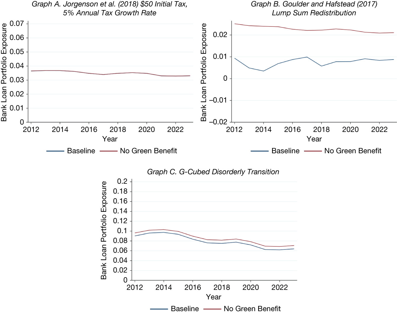
We undertake several additional extensions to deepen our understanding of banks’ transition risk exposures. The first extension addresses the fact that not all industries lose from transition policies; green industries may actually benefit. In a subset of GE models that feature benefiting industries, we evaluate the importance of bank lending to these industries. We find that banks’ exposures increase by about 1 percentage point when banks are unable to benefit from improved performance of green industries following transition policies.
Given that emissions are often used as a proxy for banks’ exposures to transition risk, we compare our exposure measures with bank-level emissions funding. We find that banks’ emissions funding explains only up to 60% of the variation in our exposure measure, suggesting that emissions alone may not fully capture transition risks. In other words, our exposure measure based on GE model estimates accounts for additional factors beyond emissions, such as forward-looking risks and industry spillovers.
Finally, we evaluate the assumption that banks maintain a static portfolio of credit exposures. Assessing this assumption is important because portfolio reallocation in response to climate-related shocks could attenuate or amplify the exposures we measure. Using difference-in-differences analyses, we find mixed evidence across GE models. Highly exposed banks reduce lending to the brownest industries after the Paris Agreement under some models, while responses are muted under others; a similar pattern holds for banks that sign the Net-Zero Banking Alliance. At the same time, borrowers in the brownest industries disproportionately switch to nonsignatory banks, suggesting that observed changes in exposures reflect banks’ management of transition risks. Taken together, our results offer some support for the static portfolio assumption. More generally, our evidence showing that banks’ responses operate mainly through reductions in lending to brown industries suggests that our bank exposure estimates can be interpreted as an upper bound on banks’ exposures to transition risks.
Our article is related to the emerging literature on the vulnerability of the financial system (e.g., Clerc, Bontemps-Chanel, Diot, Overton, Soares de Albergaria, Vernet, and Louardi, (Reference Clerc, Bontemps-Chanel, Diot, Overton, de Albergaria, Vernet and Louardi2021), European Central Bank (2023), Jung, Engle, and Berner (Reference Jung, Engle and Berner2025)), in particular banks (Arseneau, Kara, and Kotidis (Reference Arseneau, Kara and Kotidis2022), Battiston, Mandel, Monasterolo, Schütze, and Visentin (Reference Battiston, Mandel, Monasterolo, Schütze and Visentin2017), and Martini, Sautner, Steffen, and Theunisz (Reference Martini, Sautner, Steffen and Theunisz2024)) to climate transition risks. Like this literature, we too find that banks’ exposures to transition risk are meaningful. In contrast to this literature, which primarily relies on emissions-based or market-implied proxies for transition risk, we build on GE estimates of economic effects from transition policies to develop a novel measure of banks’ exposures to transition risk. This difference matters because emissions are backward-looking and are only one dimension that will be affected in a transition to a low-carbon economy. GE estimates are forward-looking by construction and should capture many different facets that will be affected in that transition.Footnote 6 As we show, emissions explain only a portion of the GE estimated effects of transition policies. Further, GE estimates allow us to investigate and compare a wide range of different carbon tax policy implementations, including different tax levels and tax redistribution mechanisms.
Our article is also related to the literature on banks’ responses to climate transition policies/risks (e.g., Antoniou, Delis, Ongena, and Tsoumas (Reference Antoniou, Delis, Ongena and Tsoumas2026), Delis, de Greiff, de Greiff, Iosifidi, and Ongena (Reference Delis, de Greiff, de Greiff, Iosifidi and Ongena2019), Ivanov, Kruttli, and Watugala (Reference Ivanov, Kruttli and Watugala2024), and Laeven and Popov (Reference Laeven and Popov2023)). Like these studies, which find weak bank responses, we too find that U.S. banks’ responses to the Paris Agreement and the signing of the Net-Zero Alliance were limited.Footnote 7 Also, the response appears to be focused on a reduction in their exposure to borrowers in brown industries.
The rest of the article is organized as follows: The next section presents our data sources and describes our methodology. That section also characterizes our sample. Section III presents our results on banks’ exposures to transition risks, as well as the results of a set of robustness tests we carry out. Section IV examines whether banks are managing their transition risk exposures. Section V concludes with some final remarks.
II. Data, Methodology, and Sample Characterization
A. Data Sources
Our main data sources are i) the Federal Reserve’s Y-14 and Y-9C databases, ii) the industry estimates associated with climate transition policies from Jorgenson et al. (Reference Jorgenson, Goettle, Ho and Wilcoxen2018), Goulder and Hafstead (Reference Goulder and Hafstead2017) and Bertram et al. (Reference Bertram, Boirard, Edmonds, Fernando, Gayle, Hurst, Liu, McKibbin, Payerols, Richters and Schets2022), and iii) Trucost data on carbon emissions. The FR Y-14Q data contains quarterly information on various asset classes, capital components, and income components for a subset of bank holding companies (BHCs) and intermediate holding companies (IHCs). These include any top-tier BHC or IHC that has $50 billion or more in total consolidated assets, as well as any other bank that is or has ever been subject to the Federal Reserve’s stress tests.Footnote 8
We use the corporate loan schedule (H.1) which contains loan-level information on loans with a commitment of $1 million or more issued by the reporting bank. We include four types of loans, defined by their line numbers on schedule HC-C of the FR Y-9C reports: C&I loans to U.S. addresses (Y-9C item 4.a), loans secured by owner-occupied nonfarm nonresidential properties (Y-9C item 1.e(1)), loans to finance agricultural production (Y-9C item 3), and other leases (Y-9C item 10.b).Footnote 9 Overall, the loans reported in the data account for about two-thirds of all C&I lending volume.
We focus on loans originated between 2012:Q3 and 2023:Q1 across 42 unique banks. We consider both drawn and undrawn commitments in our analysis. We complement this data with bank-level data, including bank assets and total C&I lending, from Y-9C reports.
The data on industry effects of climate transition policies come from three sources. The first source is Jorgenson et al. (Reference Jorgenson, Goettle, Ho and Wilcoxen2018), who estimate industry-level changes in output from carbon taxes using the Intertemporal General Equilibrium Model (IGEM).Footnote 10 The second source is Goulder and Hafstead (Reference Goulder and Hafstead2017), who estimate industry-level changes in profits induced by carbon taxes using the Environment-Energy-Economy (E3) model. The third source is the industry-output estimates for the U.S. generated by the G-Cubed model from the climate scenarios adopted by the Network for Greening the Financial System (NGFS). While there exist other GE models examining the economic effects of climate transition risk, such as that in Golosov et al. (Reference Golosov, Hassler, Krusell and Tsyvinski2014), we focus on Jorgenson et al. (Reference Jorgenson, Goettle, Ho and Wilcoxen2018), Goulder and Hafstead (Reference Goulder and Hafstead2017), and Bertram et al. (Reference Bertram, Boirard, Edmonds, Fernando, Gayle, Hurst, Liu, McKibbin, Payerols, Richters and Schets2022) because they provide industry-level information. We provide more detail on each of these models in Section III.
Our last data source is Trucost data on carbon emissions. Trucost provides information on greenhouse gas emissions (in millions of tons), which it collects from a variety of sources, including annual reports and firm disclosures in the Carbon Disclosure Project (CDP). Trucost also estimates emissions for nondisclosing firms when possible. Trucost reports emissions for three different categories based on the Greenhouse Gas Protocol (https://ghgprotocol.org/). We focus on scope 1 emissions, which are the direct emissions from establishments controlled by the company.Footnote 11
We use industry-level scope 1 emissions, computed for the average firm in the industry (weighted by the firm’s total assets from Compustat).Footnote 12 To address time variation in the availability of data on carbon emissions, we follow Ilhan et al. (Reference Ilhan, Sautner and Vilkov2021) and restrict the sample to firms in the S&P 500. We compute bank carbon emissions funding as the average of each borrower’s industry-level emissions, weighted by the amount of lending to that borrower. We use the finest feasible North American Industry Classification System (NAICS) industry classification. We also estimate bank emission intensity, which we calculate as bank emissions funding scaled by bank total assets.
B. Methodology
We use industries’ estimates of changes induced by climate-related policies from Jorgenson et al. (Reference Jorgenson, Goettle, Ho and Wilcoxen2018), Goulder and Hafstead (Reference Goulder and Hafstead2017), and Bertram et al. (Reference Bertram, Boirard, Edmonds, Fernando, Gayle, Hurst, Liu, McKibbin, Payerols, Richters and Schets2022) to measure banks’ exposures to transition risks. Each of these sources provides information on the expected reduction in industries’ profits or output generated by GE models.Footnote 13 Next, we match the industry-level estimates with bank loans in the Y-14 based on the crosswalks provided in Tables B.1, B.2, and B.3 in the Supplementary Material.Footnote 14
We then use the data to evaluate banks’ exposures to transition risks. Toward that end, we compute the decrease in the value of bank loan portfolios that would occur if loan values were to drop by the reduction in output or profits from the GE model estimates:

$ {Exposure}_{b,t}^P $
 is the exposure of bank
$ b $
 to transition risk at time
$ t $
 under policy scenario
$ P. $
 $ {Markdown}_j^P $
 is the expected percentage drop in output or profits for industry
$ j $
 under policy
$ P. $
 For simplicity, in our baseline analysis we assume that loan values will decline proportionally to the drop in the expected output or profits of the borrower’s industry. Lastly,
$ {w}_{b,j,t} $
 is the share of bank
$ {b}^{\prime }s $
 outstanding credit at time
$ t $
 granted to industry
$ j $
 .
Note that because we build on the GE estimates of transition policies, our approach does not capture individual firms’ responses to those policies.Footnote
15 Also, following the standard approach of stress testing (e.g., Hirtle and Lehnert (Reference Hirtle and Lehnert2015)), we assume that the industry composition of a bank’s loan portfolio is constant over time. This implicitly assumes that when a loan matures, the bank will either refinance it or extend a loan to another borrower in the same industry.
$ {Exposure}_{b,t}^P $
 can therefore be interpreted as the percentage drop in the value of a bank’s loan portfolio if a climate transition policy is enacted, conditional on the allocation of loans by industry at time
$ t $
 .Footnote
16
Our baseline measure is intentionally simple, making it easy to interpret, but it abstracts from several features that are useful to consider in richer settings. We therefore extend it along three dimensions. First, we put greater weight on industries most adversely affected by transition risks by assuming an extreme case in which loans to the most exposed industries lose their entire value (Section III.B.1). Second, because our baseline measure allows banks to benefit from improved performance in green industries, we construct a variant that shuts down this upside channel to isolate the losses from adversely affected industries (Section III.B.2). Third, we incorporate nonlinearities in banks’ loan exposures by drawing on supervisory Y-14 data on expected losses from default to derive a more refined bank exposure measure (Section III.B.3).
Another source of nonlinearity not captured in the GE model estimates we rely upon is economy-wide shocks that could cause default risk to rise disproportionately. We ascertain the importance of these shocks building on the 2008 GFC and the 2014–2016 oil price shock (Section III.C.). We also undertake several exercises to establish the soundness of our exposure estimates. For example, we investigate to what extent our exposure estimates are driven by banks’ contemporaneous funding of carbon emissions to assess the benefits of relying on the GE economic estimates of transition policies (Section III.D.4). Finally, we build on the Paris Agreement and the signing of the Net-Zero Alliance to ascertain banks’ constant loan portfolio composition assumption (Section IV).
C. Sample Characterization
After we merge the Y-14 data with the industry-level effects of climate policy measures, we are left with a bank-quarterly panel with 1340 observations from 2012:Q3 until 2023:Q1. Table 1 reports summary statistics, with variable descriptions provided in Table B.4 in the Supplementary Material. Banks’ exposures vary across the three models we consider and, within each model, across the policy scenarios. Looking at the Jorgenson et al. (Reference Jorgenson, Goettle, Ho and Wilcoxen2018) measures, we see that banks are more exposed to policies with higher carbon tax rates and higher tax growth rates. In the Goulder and Hafstead (Reference Goulder and Hafstead2017) model, a corporate tax cut seems to be the most favorable tax redistribution scheme for banks. Finally, in the Bertram et al. (Reference Bertram, Boirard, Edmonds, Fernando, Gayle, Hurst, Liu, McKibbin, Payerols, Richters and Schets2022) model, the orderly and disorderly transition scenarios have higher exposures for banks than the current policy. We take a close look at banks’ exposures to transition risks as captured by these models in the next section.

TABLE 1 Long description
The table contains 24 rows and 7 columns. The columns are labeled: Variable Name, Mean, Std. Dev., 10 P, 50 P, 90 P, and Count.
Key data rows include:
* Jorgenson 25 d tax, 1 p growth: Mean 0.01, Std. Dev. 0.00, 10 P 0.01, 50 P 0.01, 90 P 0.02, Count 1,340.
* Jorgenson 50 d tax, 5 p growth: Mean 0.04, Std. Dev. 0.01, 10 P 0.03, 50 P 0.03, 90 P 0.04, Count 1,340.
* Goulder corporate tax cut: Mean minus 0.02, Std. Dev. 0.06, 10 P minus 0.05, 50 P minus 0.00, 90 P 0.00, Count 1,340.
* N G F S orderly transition: Mean 0.08, Std. Dev. 0.05, 10 P 0.02, 50 P 0.07, 90 P 0.14, Count 1,340.
* N G F S disorderly transition: Mean 0.08, Std. Dev. 0.05, 10 P 0.02, 50 P 0.08, 90 P 0.14, Count 1,340.
* Emissions (m m tons): Mean 5.96, Std. Dev. 5.66, 10 P 1.78, 50 P 4.60, 90 P 11.15, Count 1,130.00.
* Emission intensity: Mean 0.04, Std. Dev. 0.05, 10 P 0.00, 50 P 0.02, 90 P 0.07, Count 1,122.00.
* ln(assets): Mean 19.42, Std. Dev. 1.06, 10 P 18.33, 50 P 19.05, 90 P 21.36, Count 1,332.
* Loans/assets: Mean 0.48, Std. Dev. 0.21, 10 P 0.14, 50 P 0.54, 90 P 0.71, Count 1,332.
* Leverage: Mean 0.89, Std. Dev. 0.03, 10 P 0.86, 50 P 0.89, 90 P 0.92, Count 1,332.
* Noninterest income/net income: Mean 2.66, Std. Dev. 8.65, 10 P 0.92, 50 P 1.82, 90 P 5.31, Count 1,332.
* The final row indicates the total number of observations is 1,340.
III. Banks’ Exposure to Transition Risks
In this section, we first describe the GE models used to estimate banks’ exposures to transition risks, and examine the time series of those exposures. Next, we investigate how banks’ exposures vary with some assumptions we make in our baseline analysis. After that, we investigate the implications of the economic conditions at the time when transition policies are introduced. We end the section with some robustness tests.
A. Banks’ Transition Risk Exposures: Baseline Analysis
We begin by computing each bank’s exposure measure for each policy scenario explored by the three models at the quarterly level. Next, we smooth the measures at an annual frequency and plot the time series of the average bank’s exposure.Footnote 17
1. Building on Jorgenson et al. (Reference Jorgenson, Goettle, Ho and Wilcoxen2018) Carbon Taxes
Our first analysis of banks’ exposures to transition risks uses the results of the IGEM-N provided in Jorgenson et al. (Reference Jorgenson, Goettle, Ho and Wilcoxen2018).Footnote
18 The authors produce estimates of the impact of carbon taxes on output for 36 industries for several initial tax levels, annual tax growth rates, and methods of recycling the income back into the economy.Footnote
19 Their policies aim at implementing the carbon trajectory necessary to meet the Paris Agreement goals or the U.S. EPA projections under scenarios developed by the Mcfarland et al. (Reference Mcfarland, Fawcett, Morris, Reilly and Wilcoxen2018). The estimated adverse impact of their policies on GDP is economically significant, ranging from 0.7% to 2%. Under their policies, the tax is instated in 2020, and grows from 2020 until 2050, so the exposure measure can be seen as the reduction in the value of a bank’s loan portfolio from time
$ t $
 until 2050.
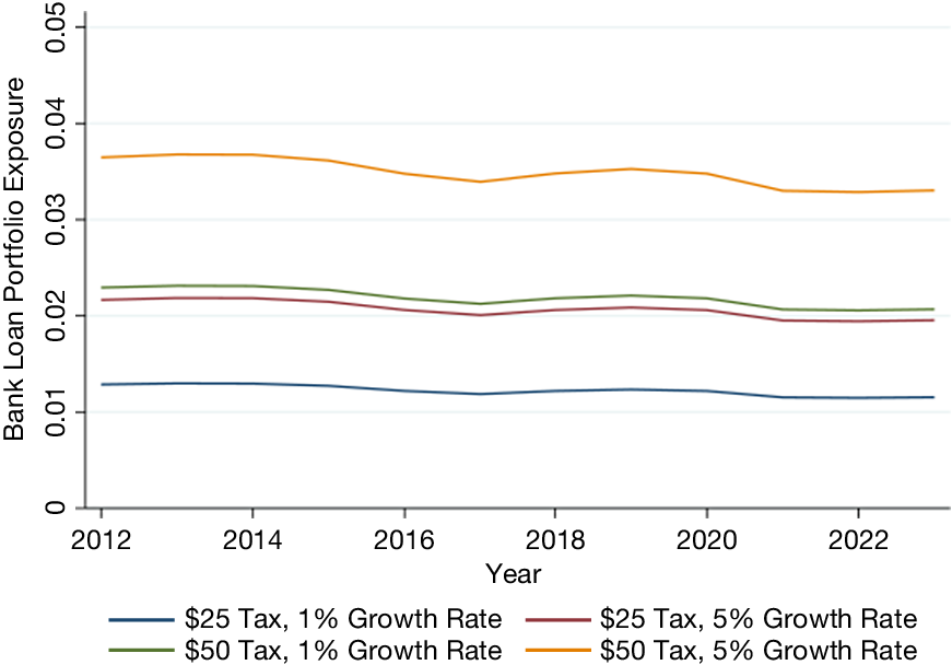
We focus on output change estimates for different initial tax levels and annual tax growth rates, where the income is recycled as a lump-sum redistribution.Footnote 20 As we can see from Figure 1, banks’ exposures based on Jorgenson et al. (Reference Jorgenson, Goettle, Ho and Wilcoxen2018) are persistent over time. The $50 initial tax rate and 5% growth rate scenario, where both the initial tax and growth rate are the highest, has the largest estimated exposure. Here, we expect that the loan portfolio of the average bank would lose about 3.5% of its value. Figure B.1 in the Supplementary Material plots the time series evolution of the average bank’s exposure based on a second set of policies (lump-sum redistribution, capital tax cut, and labor tax cut).Footnote 21
Figure 1 shows exposure to transition risks based on model estimates from Jorgenson et al. (Reference Jorgenson, Goettle, Ho and Wilcoxen2018) over time. The exposure is calculated as the percentage decrease in a bank’s loan portfolio if loan values drop the same amount as the industry-output reduction estimated in Jorgenson et al. (Reference Jorgenson, Goettle, Ho and Wilcoxen2018). Plots show the average exposure measures across banks, weighted by a bank’s total assets. Bank-level exposures are computed using the Y14 loan-level data. All scenarios assume the carbon tax is redistributed as a lump sum. Industries are defined by the authors of the referenced paper. Data are smoothed at the annual frequency and are from 2012 until 2023.

FIGURE 1 Long description
The X axis represents Year from 2012 to 2023. The Y axis represents Bank Loan Portfolio Exposure with a scale from 0 to 0.05 in increments of 0.01. Four distinct lines represent different tax and growth rate scenarios.
* The bottom line (blue) represents a $25 Tax with a 1 percent Growth Rate. It maintains a steady position just above 0.01 throughout the period.
* The second line from the bottom (maroon) represents a $25 Tax with a 5 percent Growth Rate. It starts slightly above 0.02 and shows a very gradual decline toward 0.02 by 2023.
* The third line from the bottom (green) represents a $50 Tax with a 1 percent Growth Rate. It tracks closely above the maroon line, starting near 0.023 and ending near 0.021.
* The top line (orange) represents a $50 Tax with a 5 percent Growth Rate. This scenario shows the highest exposure, starting near 0.037, dipping slightly in 2017, peaking again in 2019, and ending near 0.033.
All four lines exhibit a similar horizontal trend with minor dips around 2017 and 2021, indicating that higher initial taxes and higher growth rates correlate with higher portfolio exposure.
2. Building on Goulder and Hafstead (Reference Goulder and Hafstead2017) Carbon Taxes
We use Goulder and Hafstead (Reference Goulder and Hafstead2017) to obtain our second estimates of banks’ exposures to climate transition risk. Goulder and Hafstead (Reference Goulder and Hafstead2017) use the E3 model to examine how alternative ways to redistribute carbon tax revenues affect firms and households. Like IGEM-N, it is a multiperiod GE model. However, it is not possible to directly compare banks’ exposures under the two models. For instance, while Jorgenson et al. (Reference Jorgenson, Goettle, Ho and Wilcoxen2018) does not include a renewable energy industry, Goulder and Hafstead (Reference Goulder and Hafstead2017) includes a nonfossil electricity generation sector which benefits from carbon taxes. Additionally, while Jorgenson et al. (Reference Jorgenson, Goettle, Ho and Wilcoxen2018) provide estimates of changes in industry performance from 2015 until 2050, Goulder and Hafstead (Reference Goulder and Hafstead2017) provide estimates over an infinite time horizon. Their estimates assume that an unanticipated carbon tax is enacted in 2017, which grows to $20 per ton of carbon emissions by 2019. After that, the tax increases in real terms by 4% annually until 2048, when it reaches $60 per ton.
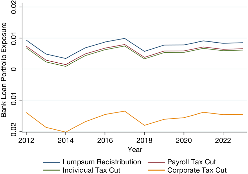
We build on Goulder and Hafstead (Reference Goulder and Hafstead2017) estimates of changes in U.S. profits for 35 industries from the carbon tax.Footnote 22 Figure 2, which plots the time series evolution of the average bank’s exposure, also shows little variation in banks’ exposure over time. The exposure estimates based on the Goulder and Hafstead (Reference Goulder and Hafstead2017) model are especially low. The loan portfolio value for the average bank is expected to fall by around 1% under the first three scenarios (a lump-sum redistribution, a payroll tax cut, and an individual income tax cut). Interestingly, when a corporate tax cut is introduced, the exposure is negative (−1.5%), meaning that the average bank would benefit from the policy, largely because profits increase for 20 out of the 35 industries.
Figure 2 shows exposure to transition risks based on model estimates from Goulder and Hafstead (Reference Goulder and Hafstead2017) over time. The exposure is calculated as the percentage decrease in a bank’s loan portfolio if loan values drop the same amount as the industry-profits reduction estimated by Goulder and Hafstead (Reference Goulder and Hafstead2017). Plots show the average exposure measures across banks, weighted by a bank’s total assets. Bank-level exposures are computed using the Y14 loan-level data. All scenarios assume a $20 initial tax and 4% annual tax growth rate. Industries are defined by the authors of the referenced paper. Data are smoothed at the annual frequency and are from 2012 until 2023.

FIGURE 2 Long description
The x-axis is labeled Year and ranges from 2012 to 2023. The y-axis is labeled Bank Loan Portfolio Exposure and ranges from negative 0.02 to 0.02 in increments of 0.01. Four lines represent different scenarios.
* Lumpsum Redistribution (blue line) is the highest, starting near 0.01 in 2012, dipping in 2014, peaking near 0.01 in 2017, and ending just below 0.01 in 2023.
* Payroll Tax Cut (maroon line) follows a similar trend but is lower, staying between 0 and 0.01.
* Individual Tax Cut (green line) is slightly below the Payroll Tax Cut line, following the same fluctuations.
* Corporate Tax Cut (orange line) is the only series in the negative range, starting near negative 0.015, reaching a low point near negative 0.02 in 2014, and ending near negative 0.015 in 2023.
All lines show a sharp dip in 2018 before recovering slightly.
3. Building on Bertram et al. (Reference Bertram, Boirard, Edmonds, Fernando, Gayle, Hurst, Liu, McKibbin, Payerols, Richters and Schets2022) Scenarios
Last, we use the G-Cubed model industry-level estimates of the Bertram et al. (Reference Bertram, Boirard, Edmonds, Fernando, Gayle, Hurst, Liu, McKibbin, Payerols, Richters and Schets2022) scenarios. The G-Cubed is a GE model that provides information on both macroeconomic and environmental outcomes in the context of the transition to a net-zero economy. We consider estimates from the G-Cubed U.S. 12-sector model.Footnote 23
In Bertram et al. (Reference Bertram, Boirard, Edmonds, Fernando, Gayle, Hurst, Liu, McKibbin, Payerols, Richters and Schets2022), the carbon tax is endogenously estimated to achieve different climate goals by 2050. In one scenario, current policies remain in place (modeled as a $3.72 carbon tax instated in 2021 that grows nonlinearly to $26.50 in 2050). In another scenario, there is an “orderly transition,” with the adoption of the necessary policy mix to achieve net-zero carbon emissions by 2050. Here, a $16.75 carbon tax is implemented in 2021 that grows nonlinearly to $119.14 in 2050, with tax proceeds used to invest in infrastructure and pay down government debt. Finally, there is a “delayed transition” scenario, where the policy is adopted in 2031 to limit the end-of-century temperature rise to below 2 degrees. For this scenario, no carbon tax is in place until 2030. At that time, a $31.52 carbon tax is enacted that grows nonlinearly to $121.97 in 2050, and the proceeds are paid to households as a lump-sum dividend.
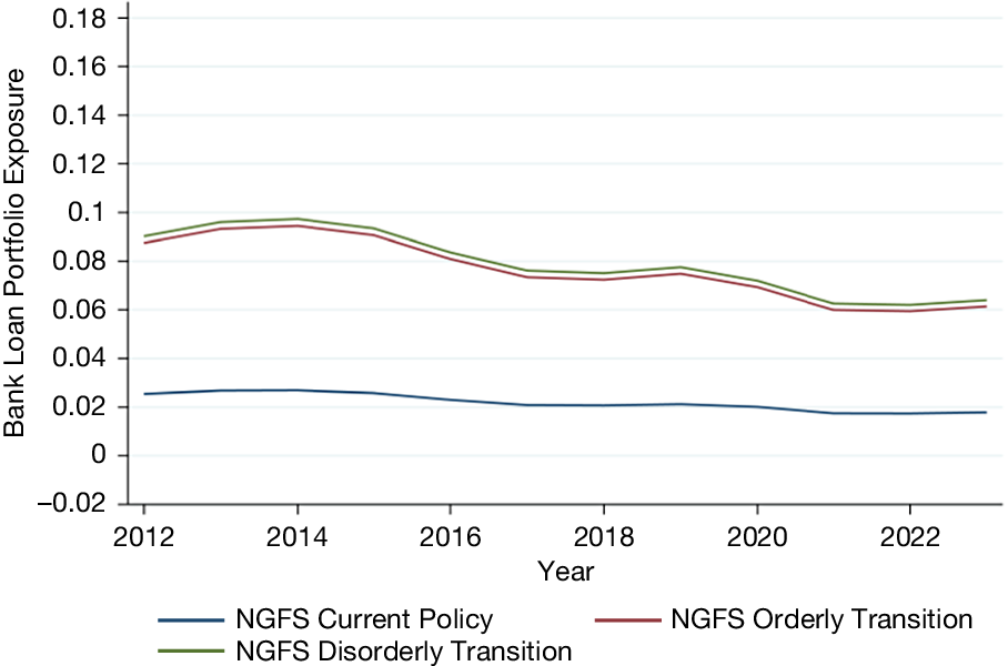
Figure 3 plots the time series of the average bank’s exposure under the three scenarios from Bertram et al. (Reference Bertram, Boirard, Edmonds, Fernando, Gayle, Hurst, Liu, McKibbin, Payerols, Richters and Schets2022). Exposures are much higher than the estimates based on Jorgenson et al. (Reference Jorgenson, Goettle, Ho and Wilcoxen2018) and Goulder and Hafstead (Reference Goulder and Hafstead2017). In the orderly transition, the average bank’s loan value decreases by about 6% as of 2023, and in the disorderly transition, it decreases by about 6.5%. Exposures based on the two scenarios have fallen by about 3 percentage points since 2014, primarily driven by increased lending to the “services” sector, which benefits from the transition according to the model. On the other hand, the exposure is about 2% under the current policy scenario based on banks’ loan portfolios as of 2023. Banks’ exposures are highest (lowest) under the disorderly (current) policy scenarios, respectively.Footnote 24 The idea that more stringent policies generate higher bank exposures is also present in the other models and confirmed in regression analysis.Footnote 25
Figure 3 shows exposure to transition risks based on model estimates from G-Cubed over time. The exposure is calculated as the percentage decrease in a bank’s loan portfolio if loan values drop the same amount as the industry-output reduction estimated by Bertram et al. (Reference Bertram, Boirard, Edmonds, Fernando, Gayle, Hurst, Liu, McKibbin, Payerols, Richters and Schets2022). Plots show the average exposure measures across banks, weighted by a bank’s total assets. Bank-level exposures are computed using the Y14 loan-level data. Industries are as defined by the G-Cubed. Data are smoothed at the annual frequency and are from 2012 until 2023.

FIGURE 3 Long description
The X-axis represents Year from 2012 to 2023 in two-year increments. The Y-axis represents Bank Loan Portfolio Exposure with a scale from negative 0.02 to 0.18 in increments of 0.02.
Three data series are plotted:
* N G F S Disorderly Transition (green line): This is the highest line, starting near 0.09 in 2012, peaking at approximately 0.10 in 2014, and then trending downward to roughly 0.06 by 2023.
* N G F S Orderly Transition (red line): This line follows a nearly identical path to the Disorderly Transition line but sits slightly lower, starting at 0.08 and ending just above 0.06.
* N G F S Current Policy (blue line): This is the lowest line, showing a much flatter trend. It starts at approximately 0.025, remains relatively stable with a very slight decline, and ends just below 0.02 in 2023.
A legend at the bottom identifies the three scenarios.
B. Understanding Banks’ Baseline Risk Exposures
In this section, we present three variations to our baseline exposure measure. This will allow us to better understand our baseline measure, as well as the importance of different assumptions made to construct it.
1. Banks’ Exposures to the Most Brown Industries
There may be nonlinear effects of transition risks on bank payoffs. For instance, brown industries could be disproportionally affected in the transition. To this end, we consider a stress scenario in which loans to the most adversely affected industries lose their entire value. For all other industries, losses are assumed to be proportional to declines in the borrower’s industry output (or sales).Footnote 26 The bank’s exposure under stress is defined as:

where
$ Exposure\ Under\;{Stress}_{b,t}^P $
 is the exposure for bank
$ b $
 at time
$ t $
 under policy
$ P $
 . We define the industries most exposed to transition risks (i.e., the most brown industries) as those in the top one or top two deciles of transition risk distribution across industries.
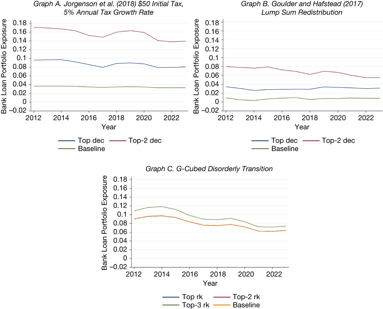
The time series of banks’ exposures to the most brown industries are displayed in Figure 4. Graph A displays the results for the Jorgenson et al. (Reference Jorgenson, Goettle, Ho and Wilcoxen2018) model. The estimates are considerably higher using the
$ Exposure\ Under\ Stress $
 than with the baseline
$ Exposure $
 measure. The expected drop in bank loan portfolio values increases by about 4.5 percentage points when assuming that the top decile of industries lose all of their value, and an additional 6 percentage points when assuming that the top two deciles of industries lose all of their value. Note that these estimates have declined by 1–3 percentage points over the past 10 years, consistent with banks gradually reducing their exposures to the most brown industries.
Figure 4 shows exposures to transition risks for the most brown industries from model estimates of industry-level exposures to transition risks for the scenarios yielding the highest exposures over time. Estimates from Jorgenson et al. (Reference Jorgenson, Goettle, Ho and Wilcoxen2018), Goulder and Hafstead (Reference Goulder and Hafstead2017), and Bertram et al.(Reference Bertram, Boirard, Edmonds, Fernando, Gayle, Hurst, Liu, McKibbin, Payerols, Richters and Schets2022) are shown in Graphs A, B, and C respectively. The exposure is calculated as the percentage decrease in a bank’s loan portfolio if loan values for all loans to the most brown industries had zero value, and loans to all the other industries decreased by the same amount as the output reduction in the appropriate model. For Jorgenson et al. (Reference Jorgenson, Goettle, Ho and Wilcoxen2018) and Goulder and Hafstead (Reference Goulder and Hafstead2017), the most brown industries are those in the top two deciles of exposure to transition risks, and for Bertram et al. (Reference Bertram, Boirard, Edmonds, Fernando, Gayle, Hurst, Liu, McKibbin, Payerols, Richters and Schets2022), the most brown industries are either the top ranked, top two ranked, or top three ranked exposed to transition risks. Industries are defined by the authors of the referenced paper. Data are smoothed at the annual frequency and are from 2012 until 2023.

FIGURE 4 Long description
A three-panel set of line graphs. All graphs share a horizontal X axis for Year from 2012 to 2023 and a vertical Y axis for Bank Loan Portfolio Exposure ranging from negative 0.02 to 0.18.
Graph A, titled Jorgenson et al. 2018, 50 dollar Initial Tax, 5 percent Annual Tax Growth Rate, shows three lines. The Top-2 dec line starts highest at 0.17, fluctuating downward to 0.14. The Top dec line starts at 0.10 and ends near 0.08. The Baseline remains flat near 0.04.
Graph B, titled Goulder and Hafstead 2018, Lump Sum Redistribution, shows three lines at lower exposure levels. The Top-2 dec line starts at 0.08 and trends down to 0.06. The Top dec line stays relatively flat near 0.03. The Baseline is flat near 0.01.
Graph C, titled G-Cubed Disorderly Transition, shows four lines. The Top-3 rk line starts at 0.11, peaks at 0.12 in 2014, then declines to 0.07. The Top-2 rk, Top rk, and Baseline lines are closely clustered, starting at 0.09 and declining to approximately 0.06 by 2023.
Graph B shows that the
$ Exposure\ Under\ Stress $
 is about 2 percentage points higher than the baseline exposure when the top-decile industry loses all of its value under Goulder and Hafstead (Reference Goulder and Hafstead2017), and by an additional 2 percentage points when assuming the top two deciles lose all of their value. For the NGFS model, we see from Graph C that the
$ Exposure\ Under\ Stress $
 measure is almost identical to the baseline when assuming the two most brown industries default in the “disorderly transition” scenario.Footnote
27 This similarity reflects the fact that the NGFS scenarios already imply losses comparable in magnitude to those assumed in our severe scenario. In the NGFS disorderly scenario, output in gas extraction and utilities (the most brown industry) falls by 100% by 2050, and output in coal (the second most brown industry) falls by about 96%, leaving little additional loss to be projected under our Exposure Under Stress measure. When we assume the top three ranked industries lose their entire value, banks’ loan portfolio values are expected to decline by an additional 1 percentage point as of 2023.
These results show that banks’ loan portfolios in 2023 would drop by about 14% under the extreme assumption that the 20% of industries most affected by climate transition risks, according to Jorgenson et al. (Reference Jorgenson, Goettle, Ho and Wilcoxen2018), completely lose their value, although they are smaller under Goulder and Hafstead (Reference Goulder and Hafstead2017) and Bertram et al. (Reference Bertram, Boirard, Edmonds, Fernando, Gayle, Hurst, Liu, McKibbin, Payerols, Richters and Schets2022).Footnote 28 Overall, these exposures have decreased by about 2–4 percentage points since 2012, further suggesting that banks have been reducing their exposure to the most brown industries.
2. Evaluating the Benefits of Green Industries’ Exposures
Our baseline exposure measure allows banks to benefit from improved performance in green industries following the implementation of transition policies. In this section, we consider a variant that shuts down this channel. Specifically, when constructing the exposure measure, we bound the increase in industry output or profits at zero. This variant both isolates the role of gains from green industries and reflects the asymmetric nature of loan payoffs, which limits banks’ ability to benefit from upside realizations.
Figure 5 shows the time series of banks’ exposure without any benefit from green industries. In the Goulder and Hafstead (Reference Goulder and Hafstead2017) and Bertram et al. (Reference Bertram, Boirard, Edmonds, Fernando, Gayle, Hurst, Liu, McKibbin, Payerols, Richters and Schets2022) models, exposures increase by about 1 percentage point once banks no longer benefit from lending to green borrowers.Footnote 29 No change is observed for the Jorgenson et al. (Reference Jorgenson, Goettle, Ho and Wilcoxen2018) model because there is no sector that greatly benefits from transition policies in their model, which highlights how different model assumptions can drive exposure estimates. Overall, our results suggest that gains from green industries matter but are quantitatively modest, especially relative to the risk exposure coming from brown industries.
Figure 5 shows exposures to transition risks from model estimates of industry-level exposures over time. Estimates from Jorgenson et al. Reference Jorgenson, Goettle, Ho and Wilcoxen2018, Goulder and Hafstead (Reference Goulder and Hafstead2017) and Bertram et al. (Reference Bertram, Boirard, Edmonds, Fernando, Gayle, Hurst, Liu, McKibbin, Payerols, Richters and Schets2022) are shown in Graphs A, B, and C respectively. Loan exposures are calculated as described in section III.B.2. We cap loan balances so they cannot increase above their current day value. Exposures are adjusted so banks cannot benefit from improved performance by green industries following transition risks. Industries are defined by the authors of the referenced paper. Data are smoothed at the annual frequency and are from 2012 until 2023.

FIGURE 5 Long description
A three-panel set of line graphs. All graphs share a horizontal x-axis for Year, ranging from 2012 to 2023, and a vertical y-axis for Bank Loan Portfolio Exposure. Each graph contains two lines: a blue line for Baseline and a red line for No Green Benefit.
* Graph A, Jorgenson et al. 2018, 50 dollar Initial Tax, 5 percent Annual Tax Growth Rate: The y-axis ranges from 0 to 0.07. Both the Baseline and No Green Benefit lines are nearly identical, showing a stable trend around 0.035 with a very slight decline toward 2023.
* Graph B, Goulder and Hafstead 2018, Lump Sum Redistribution: The y-axis ranges from negative 0.02 to 0.02. The red No Green Benefit line starts at approximately 0.025 and shows a very gradual decline. The blue Baseline line starts lower at approximately 0.01, dips in 2014, and then fluctuates upward to end near 0.01 in 2023.
* Graph C, G-Cubed Disorderly Transition: The y-axis ranges from 0 to 0.2. Both lines show a similar trajectory, peaking around 2014 before entering a steady decline. The red No Green Benefit line remains consistently higher than the blue Baseline line throughout the period, ending at approximately 0.07 compared to the baseline’s 0.06.
3. Banks’ Exposures Accounting for Nonlinearity in Loan Payoffs
Section III.B.1 provides a simple way to account for banks’ nonlinear exposure to default risk across industries. There, we assume complete losses on loans to the most exposed industries to highlight the potential magnitude of exposure under a severe scenario. In this section, we complement the previous analysis by using expected loss estimates to directly capture the nonlinear effect of transition risks on loans’ payoffs.
Since bank loan payoffs are typically nonlinearly related to a borrower’s performance, we use the Y-14’s data on LGD, PD, and borrower sales to estimate the relationship between expected loan losses and sales for each industry. Specifically, we begin by sorting expected loan losses (PD
$ \times LGD $
 ) into sales deciles, within industry, where the industries are defined according to the GE model. Next, we run the following regression, separately for each industry
$ j $
 and year
$ t $
 :

where
$ {Losses}_i $
 represent the expected losses for loan
$ i $
 , and
$ {d}_i $
 is equal to 1 if the borrower for loan
$ i $
 was in sales decile
$ k $
 in year
$ t $
 . Whenever possible, we run regressions within 3-digit NAICS industries for each year. If this is not possible, we run regressions within 2-digit NAICS industries for each year.Footnote
30 Otherwise, we run regressions within the broad industries used by the GE model. We cap losses for bank
$ i $
 at 1, ensuring that losses do not exceed the full value of the loan portfolio. While we do not have information on borrowers’ leverage ratios, and therefore cannot rely on them to identify nonlinearities in default, we still account for the possibility that defaults become more likely for risky borrowers by assuming a default probability of 1 for loans with an above-average PD. For all other loans, losses are computed using the expected loss estimates from equation (3).
Finally, we combine the estimated relationship computed using equation (3) with the GE model estimates of decline in sales for each scenario to compute
$ NLExposure $
 , the exposure accounting for the nonlinear relationship between borrower sales and loan losses:

where
$ {w}_{b,j,t} $
 represents the share of loan amount made by bank
$ b $
 to industry
$ j $
 in quarter
$ t $
 , and
$ {\hat{Losses}}_i $
 estimates come from (3).
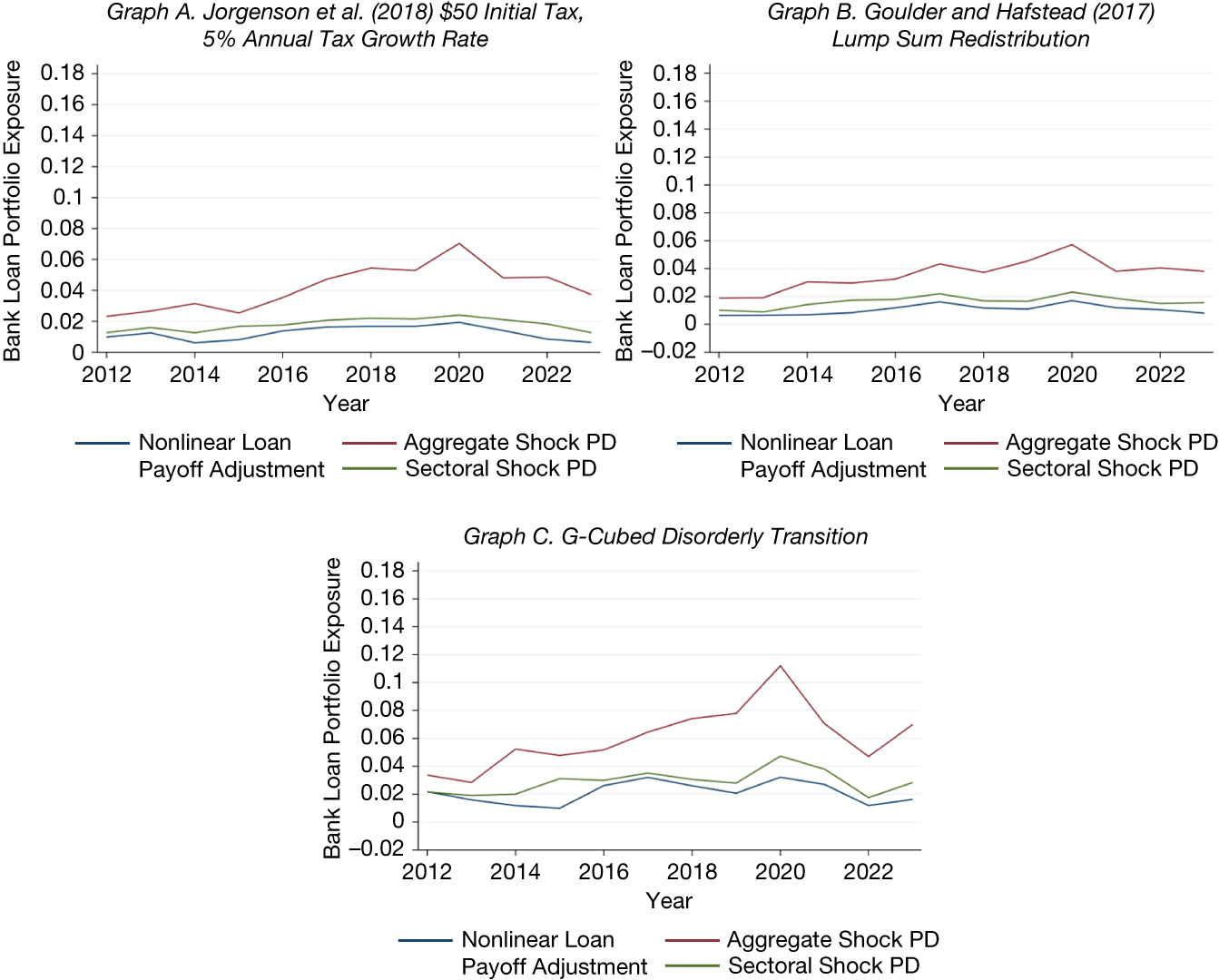
Figure 6 shows banks’ exposures adjusted for the nonlinearity of loans’ payoffs. The exposures are similar across models, ranging between 0.5% and 2% as of 2023. As of 2023, at worst, exposures adjusted for loans’ payoff nonlinearity are about the same as baseline exposures (for the same model), and at best are up to 4 percentage points lower. This is because banks typically do not lose the full value of a loan upon default in historical realizations.
Figure 6 shows exposures to transition risks adjusted for nonlinearities in the payoff structure from model estimates of industry-level exposures over time. Estimates from Jorgenson et al. (Reference Jorgenson, Goettle, Ho and Wilcoxen2018), Goulder and Hafstead (Reference Goulder and Hafstead2017), and Bertram et al. (Reference Bertram, Boirard, Edmonds, Fernando, Gayle, Hurst, Liu, McKibbin, Payerols, Richters and Schets2022) are shown in Graphs A, B, and C respectively. The exposure is calculated as the percentage decrease in a bank’s loan portfolio if we assume all loans with an above-average probability of default eventually default. For the industries that default, we adjust by the loss given default in the Y-14, and for all other industries we adjust by the total loss as estimated from a regression of borrower expected loss on sales decile indicators. For Jorgenson et al. (Reference Jorgenson, Goettle, Ho and Wilcoxen2018) and Goulder and Hafstead (Reference Goulder and Hafstead2017), the most brown industries are those in the top two deciles of exposure to carbon taxes, and for Bertram et al. (Reference Bertram, Boirard, Edmonds, Fernando, Gayle, Hurst, Liu, McKibbin, Payerols, Richters and Schets2022), the most brown industries are the three industries most exposed to climate policy. To capture the effect of a major aggregate shock, we add the rise in industry-level probabilities of default that occurred during the 2008 financial crisis (2007:Q2–2009:Q1) to the loan-level probabilities of default in the Y-14, and to capture the effect of a sectoral shock, we add the change in industry-level probabilities of default that occurred from the peak in oil prices to their bottom (i.e., 2014:Q2 until 2016:Q1) to the loan-level probabilities of default in the Y-14. Industries are defined by the authors of the referenced paper. Data are smoothed at the annual frequency and are from 2012 until 2023.

FIGURE 6 Long description
A three-panel set of line graphs labeled Graph A, Graph B, and Graph C. All graphs share a common X-axis representing Year from 2012 to 2023 and a Y-axis representing Bank Loan Portfolio Exposure ranging from -0.02 to 0.18. Each graph contains three lines: Nonlinear Loan Payoff Adjustment (blue), Aggregate Shock P D (red), and Sectoral Shock P D (green).
* Graph A. Jorgenson et al. 2018 $50 Initial Tax, 5% Annual Tax Growth Rate: The red line (Aggregate Shock) starts at 0.02, peaks at 0.07 in 2020, and ends near 0.04. The green line (Sectoral Shock) and blue line (Nonlinear Adjustment) remain lower, fluctuating between 0 and 0.02.
* Graph B. Goulder and Hafstead 2018 Lump Sum Redistribution: The red line starts at 0.02, reaches a peak of approximately 0.06 in 2020, and ends at 0.04. The green and blue lines track closely together between 0 and 0.02 throughout the period.
* Graph C. G-Cubed Disorderly Transition: This graph shows the highest volatility. The red line starts at 0.03, climbs steadily to a sharp peak of 0.11 in 2020, drops to 0.05 in 2022, and rises to 0.07 in 2023. The green and blue lines also show a peak in 2020 at approximately 0.05 and 0.03 respectively, before declining and slightly recovering.
Assuming that loan losses following transition policies resemble historical default outcomes provides a natural benchmark for estimating the impact of those policies. However, that impact may underestimate the full implementation of transition policies. Further, it may also depend on the economic conditions at the time the policies are implemented, a possibility we explicitly consider next.
C. Sensitivity of Banks’ Exposures to Shocks
The stress scenario exercise in which loans to the most adversely affected industries lose their entire value, while arguably extreme, highlights the importance of nonlinear effects on banks’ transition risk exposures. An additional dimension of nonlinearity arises from state dependence; as shown in Nagel and Purnanandam (Reference Nagel and Purnanandam2020), shocks can interact with adverse aggregate conditions, causing default risk to rise disproportionately in bad states of the economy. In light of this mechanism, the adverse effects of transition policies can be amplified during economic downturns.
To capture this state-dependent nonlinearity, we consider two types of shocks to the economy: an economy-wide shock and a shock specific to the energy sector. For the former, we use the 2008 GFC because it represents a sharp deterioration in aggregate economic conditions. For the latter, we use the 2014–2016 oil price shock. Between mid-2014 and early 2016, oil prices fell by roughly 70 percent, marking one of the three largest oil price declines since World War II and the most persistent since the supply-driven collapse of 1986 (World Bank, 2018). The prolonged and sector-specific nature of this episode makes it a natural laboratory for sustained stress in the energy sector.Footnote 31
To assess how bank exposures would change if transition policies were implemented during a downturn, we construct a counterfactual increase in default risk calibrated to the crisis episodes described in the above paragraph. Specifically, for each industry (6-digit NAICS-level), we compute the change in the PDs over each shock episode.Footnote 32 We then apply these changes to loan-level PDs in the Y-14 to estimate counterfactual bank exposures under crisis-like conditions.
For the GFC, we define the shock period based on the trough-to-peak in the aggregate default risk, which corresponds to 2007:Q2 to 2009:Q1. We take this approach because PDs, rather than business-cycle dating per se (e.g., NBER recessions), are the relevant state variable for bank loan losses. For the energy-sector shock, we define the shock period using the peak-to-trough decline in the Brent Crude Oil index, which spans 2014:Q2 to 2016:Q1 (https://fred.stlouisfed.org/graph/?g=ko34). While one could calibrate the shock using default-probability changes for a preselected set of affected industries, the oil price collapse did not impact all industries uniformly, making such a selection unclear ex ante. We, therefore, anchor the shock directly in the observed oil price decline.
Figure 6 reports the estimated exposure to transition risk under the aggregate shock (solid red line). An economy-wide downturn increases banks’ (nonlinearity-adjusted) exposures by roughly 3–5 percentage points, based on 2023 loan portfolios, with exposures reaching up to 11% in 2020 under the Bertram et al. (Reference Bertram, Boirard, Edmonds, Fernando, Gayle, Hurst, Liu, McKibbin, Payerols, Richters and Schets2022) framework. This reflects both the amplification of transition-related losses in highly exposed sectors and broader increases in default risk across less transition-exposed industries.
The effects of the sectoral shock are shown by the green line. With an energy-sector shock, exposures rise by about 1 percentage point relative to the nonlinearity-adjusted baseline. Unlike the aggregate shock, the oil price collapse did not increase default risk uniformly across industries. While transition-exposed sectors experienced higher default risk, other sectors, including some green industries, benefited from lower energy costs, muting the overall impact on exposure.
Overall, these results suggest that banks’ exposures to transition risk can be amplified when transition policies coincide with adverse aggregate economic conditions. Sectoral shocks during the transition, by contrast, have relatively smaller effects on banks’ exposures.
D. Robustness Analysis and Extensions
In this section, we present a set of robustness analyses and extensions to deepen our understanding of banks’ exposures to transition risk.
1. Within-Industry Heterogeneity
In constructing our exposure measure, we assume that bank selection of borrowers within an industry is random relative to the borrower’s transition risk. To examine this assumption, we use granular industry-level emissions data, at the 4-digit NAICS level, which allows us to examine heterogeneity in banks’ lending to high- and low-emission industries, within each sector of the GE models. To do this, we identify the highest and lowest emitting industries within each modeled sector and calculate the following ratio:

where
$ {Lending}_{it}^{Low} $
 is lending to the lowest-emitting borrowers in the GE sector and
$ {Lending}_{it}^{High} $
 is lending to the highest-emitting borrowers in the GE sector.Footnote
33 We regress this measure on bank fixed effects for each quarter in the sample.
The
$ {R}^2 $
 of these regressions based on the Jorgenson et al. (Reference Jorgenson, Goettle, Ho and Wilcoxen2018) industries are plotted in Figure B.4 in the Supplementary Material. The blue line displays the trend in the
$ {R}^2 $
 from each of these regressions over time. At most, the
$ {R}^2 $
 is 5%, indicating that most of
$ P\left({Lending}_{it}^{Low}\right) $
 is not explained by bank behavior. Also, the fitted line through the
$ {R}^2 $
 s is flat, suggesting that banks are not increasingly sorting into browner or greener borrowers within each industry over time. The red line, which displays the
$ {R}^2 $
 from a regression of
$ P\left({Lending}_{it}^{Low}\right) $
 on both bank and industry fixed effects, shows similar results.
2. Exposure Relative to Bank Capital
The results reported thus far show banks’ exposures to transition risk scaled by their assets. Given that leverage plays an important role in determining banks’ vulnerability, we also scale exposures by bank capital. Figure B.5 in the Supplementary Material displays the results scaling the exposure measure by bank capital for all three models. As expected, scaling by bank capital yields larger exposures, but it does not change the relative impact of the various policies.
3. Banks’ Exposures over the Transition Path
Our baseline estimates report the long-run impact of transition policies as of the final year in the model horizon—that is, a snapshot of the final outcome. However, one may also be interested in understanding how exposures evolve along the transition path. While most GE models we rely on do not report intermediate outcomes, the G-Cubed model provides industry-level estimates over time. We, therefore, use the G-Cubed transition paths to trace the evolution of banks’ exposures under each scenario.
The resulting exposure paths using the G-Cubed scenarios are shown in Figure B.6 in the Supplementary Material. Based on our baseline measure, while the exposures under the current policy and orderly policy are realized gradually over time, the exposure of banks under the disorderly scenario is zero until 2030. At that point, the exposure under the disorderly scenario increases more rapidly than in the other two scenarios. By contrast, when assuming the top one, two, and three most affected industries lose their entire value, exposures are realized much more quickly than in the baseline measure.
4. Banks’ Emissions Funding and Exposure to Transition Risk
Finally, thus far we have not considered carbon emissions, which are commonly used to proxy for climate transition risks. Therefore, one may wonder how our findings compare to banks’ exposures had we relied on carbon emissions. To this end, we regress our estimates on banks’ exposures on banks’ carbon emission funding and carbon emissions intensity for each policy scenario, and report the
$ {R}^2 $
 of these regressions in Table 2.

TABLE 2 Long description
The table is divided into four panels, each presenting R-squared values for Emissions and Emission intensity.
Panel A. Jorgenson et al. 2018 Tax and Growth Rate Scenarios.
* Model Scenario I ($25 Tax, 1% Growth): Emissions R-squared 0.572, Emission intensity R-squared 0.270.
* Model Scenario II ($25 Tax, 5% Growth): Emissions R-squared 0.577, Emission intensity R-squared 0.269.
* Model Scenario III ($50 Tax, 1% Growth): Emissions R-squared 0.582, Emission intensity R-squared 0.272.
* Model Scenario IV ($50 Tax, 5% Growth): Emissions R-squared 0.588, Emission intensity R-squared 0.272.
Panel B. Jorgenson et al. 2018 Redistribution Scenarios.
* Lump Sum Redistribution: Emissions R-squared 0.577, Emissions intensity R-squared 0.269.
* Capital Tax Cut: Emissions R-squared 0.595, Emissions intensity R-squared 0.297.
* Labor Tax Cut: Emissions R-squared 0.577, Emissions intensity R-squared 0.262.
Panel C. Goulder and Hafstead 2017 Redistribution Scenarios.
* Lump Sum Redistribution: Emissions R-squared 0.297, Emissions intensity R-squared 0.117.
* Corporate Tax Cut: Emissions R-squared 0.297, Emissions intensity R-squared 0.116.
* Payroll Tax Cut: Emissions R-squared 0.297, Emissions intensity R-squared 0.117.
* Individual Income Tax Cut: Emissions R-squared 0.297, Emissions intensity R-squared 0.118.
Panel D. G-Cubed Scenarios.
* Current Policy: Emissions R-squared 0.496, Emission intensity R-squared 0.254.
* Disorderly Transition: Emissions R-squared 0.411, Emission intensity R-squared 0.207.
* Orderly Transition: Emissions R-squared 0.416, Emission intensity R-squared 0.208.
Depending on the model and the scenario used, the
$ {R}^2 $
 is at least 30%, and at most 60%. Overall, it is reassuring to observe a positive correlation between our GE-based exposures and bank emissions funding; after all, industries with high emissions are expected to be more affected by the transition policies.Footnote
34 However, it is notable that at least 40% of the variation in our exposure measures is not explained by carbon emissions alone. Additionally, we examine the relationship between the industry-level emissions and industry-level exposures in Table B.11 in the Supplementary Material and find that the
$ {R}^2 $
 estimates are even lower.
IV. Do Banks Manage Transition Risks’ Exposures?
Our approach assumes that banks’ loan portfolio compositions remain constant following the implementation of carbon tax policies, consistent with standard stress-testing frameworks. Evaluating this assumption is important because portfolio reallocation in response to climate-transition policies could either attenuate or amplify the exposures we measure. Because a carbon tax has not been implemented in the United States, we instead examine this assumption by exploiting banks’ responses to two important climate-related events: the Paris Agreement and banks’ signing of the Net-Zero Banking Alliance. If banks adjust their portfolios in response to these events, the direction and magnitude of the adjustment will help assert whether our baseline estimates are closer to a lower or an upper bound.
A. Paris Agreement
We begin by investigating banks’ responses to the Paris Climate Accord. On Dec. 12, 2015, 196 nations adopted the Paris Agreement. By doing so, they agreed to enact national action plans limiting end-of-century temperature rise to at most 1.5 degrees Celsius above pre-industrial levels. These national action plans would require policy actions, such as carbon pricing or regulation, that would likely have disproportionately negative effects for industries exposed to transition risk.Footnote 35
We empirically examine whether banks with significant lending portfolios to industries exposed to transition risk changed their lending policies after the Paris Agreement. To do this, we first identify the most affected banks as the ones with high exposure to the most brown industries before the Paris Agreement. Next, we run the following regression:

where
$ Pre\hbox{-} Paris\;{Exposure}_i $
 is the exposure for bank
$ i $
 as of the quarter before the Paris Agreement (2015:Q3) and
$ {Post}_t $
 is a dummy variable which takes a value of 1 if
$ t $
 is after the Paris Agreement, and 0 otherwise.Footnote
36 We include bank-level controls (
$ {X}_{i,t} $
 ), as well as bank and time fixed effects (
$ {\gamma}_i,{\delta}_t $
 ). The exposure is policy-specific and is computed based on equation (1). The sample period is from 2012:Q3 to 2019:Q4 to isolate the effect coming from the other important event, signing of the Net-Zero Banking Alliance, which occurred in 2021. We consider the most severe policy from each model to compute the exposure, that is the $50 tax growing at 5% annually for the Jorgenson et al. (Reference Jorgenson, Goettle, Ho and Wilcoxen2018) model, carbon tax policy with lump-sum redistribution for the Goulder and Hafstead (Reference Goulder and Hafstead2017) model, and the disorderly transition for the Bertram et al. (Reference Bertram, Boirard, Edmonds, Fernando, Gayle, Hurst, Liu, McKibbin, Payerols, Richters and Schets2022) model. We expect a negative
$ \beta $
 if the affected banks reduced their exposures (compared to the control group) following the Paris Agreement.
Panel A of Table 3 reports the results. Columns 1–3 are based on the aforementioned climate models and column 4 examines the effect on the bank-level emission funding. The results are mixed. The negative coefficients in columns 1 and 3 indicate that banks reduced their exposures following the Paris Agreement. In the specification based on the Goulder and Hafstead (Reference Goulder and Hafstead2017) model (column 2), the coefficient is also negative but not statistically significant. When exposure is measured using emissions, the coefficient turns positive, although it is not statistically significant.

TABLE 3 Long description
The table is divided into three panels: Panel A on Banks’ Exposures, Panel B on Lending to the Most Brown Industries, and Panel C on Lending to the Most Green Industries. Each panel contains four numbered columns representing different models: 1 (I G E M), 2 (Goulder and Hafstead), 3 (N G F S), and 4 (Emissions).
Panel A: Banks’ Exposures
* Column 1: Pre-Paris I G E M exposure times Post Paris coefficient is -0.140 (t-stat -3.22, significant at 1%).
* Column 2: Pre-Paris Goulder exposure times Post Paris coefficient is -0.090 (t-stat -1.59).
* Column 3: Pre-Paris N G F S exposure times Post Paris coefficient is -0.175 (t-stat -3.00, significant at 1%).
* Column 4: Pre-Paris emissions times Post Paris coefficient is 0.046 (t-stat 0.75).
Panel B: Lending to the Most Brown Industries
* Column 1: Coefficient is -2.266 (t-stat -3.02, significant at 1%).
* Column 2: Coefficient is -0.044 (t-stat -0.41).
* Column 3: Coefficient is -0.261 (t-stat -2.78, significant at 1%).
* Column 4: Coefficient is -0.003 (t-stat -4.59, significant at 1%).
Panel C: Lending to the Most Green Industries
* Column 1: Coefficient is -0.042 (t-stat -0.04).
* Column 2: Coefficient is 0.231 (t-stat 3.55, significant at 1%).
* Column 3: Coefficient is 0.381 (t-stat 3.28, significant at 1%).
* Column 4: Coefficient is -0.001 (t-stat -0.27).
All models include Controls, Bank fixed effects, and Time fixed effects. Number of observations is 897 for columns 1-3 and 841 for column 4 across all panels. Within R-squared values range from 0.014 to 0.163.
In order to understand which margin—reducing brown exposure and/or increasing green exposures—banks adjust, we analyze the shares of loans to the “most brown” and “most green” industries separately. We identify the former industries as those in the top two deciles of exposure and the latter industries as those in the bottom two deciles of exposure.Footnote 37 Panel B of Table 3 shows that the affected banks reduced lending to the most brown industries, and Panel C shows that they increased lending to the most green industries, relative to the control group, following the Paris Agreement. Overall though, the change in exposure appears more driven by the decline in browner lending than an increase in greener lending.
Although the mixed evidence on portfolio rebalancing following the Paris Agreement offers some support for the static balance sheet assumption, one may wonder to what extent it derives from the declining oil prices which overlapped with the Paris Agreement. To help isolate banks’ management of their exposures to climate transition risks, we examine banks’ responses to their signing of the Net-Zero Banking Alliance.
B. Signing of Net-Zero Banking Alliance
In 2021:Q1, an international coalition of banks created the Net-Zero Banking Alliance “committed to financing ambitious climate action to transition the real economy to net-zero GHG emissions by 2050.” This provides a suitable setting to test whether banks are adjusting their lending in response to concerns about transition risks. We define the treated group as the 11 banks in the Y-14 that signed the Alliance in 2021:Q1. We focus on the sample period 2017:Q2 to 2023:Q1 to isolate the effect of the Net-Zero Banking Alliance signing. This design narrows the post-time window, and therefore, the results should be interpreted with this caveat in mind. We exclude from the sample the seven banks that signed the Alliance later. Unlike the previous analysis focusing on the Paris Agreement, what matters in this exercise is whether banks joined the Alliance or not, rather than the pre-shock exposure. This is because highly exposed banks are not really affected unless they sign the commitment.
To examine the effect of making the commitments, we regress exposure on the interaction between a bank-level variable,
$ Signatory $
 , and a time dummy variable,
$ Post $
 :

where
$ {Signatory}_i $
 takes a value of 1 if the bank signed the Net-Zero Banking Alliance, and 0 otherwise, and
$ {Post}_t $
 is a time dummy variable that takes a value of 1 if it was after the initial signing in 2021:Q1. We expect to find negative
$ \beta $
 if the signatory banks reduced their exposures relative to other banks after signing the Alliance.
Similar to our previous analysis, the results are mixed. Table 4 shows that signatory banks reduced their exposures relative to nonsignatory banks after signing the Net-Zero Banking Alliance, based on the Jorgenson et al. (Reference Jorgenson, Goettle, Ho and Wilcoxen2018) and the Bertram et al. (Reference Bertram, Boirard, Edmonds, Fernando, Gayle, Hurst, Liu, McKibbin, Payerols, Richters and Schets2022) models. The results based on the emissions measure and Goulder and Hafstead (Reference Goulder and Hafstead2017) are not statistically significant. The signs of coefficients in Panels B and C are consistent with the decline in exposure being driven by banks reducing lending to the most brown industries rather than increasing lending to the most green industries. However, the coefficients are statistically significant only under the Bertram et al. (Reference Bertram, Boirard, Edmonds, Fernando, Gayle, Hurst, Liu, McKibbin, Payerols, Richters and Schets2022) model.

TABLE 4 Long description
The table consists of three panels: Panel A on Banks’ Exposures, Panel B on Lending to the Most Brown Industries, and Panel C on Lending to the Most Green Industries. Each panel contains four columns representing different measures: Jorgenson, Goulder and Hafstead, N G F S, and Emissions.
Panel A: Banks’ Exposures
* Signatory times Post alliance interaction: Column 1 is minus 0.001 (t-stat minus 1.81); Column 2 is 0.002 (t-stat 0.41); Column 3 is minus 0.011 (t-stat minus 2.01); Column 4 is minus 0.908 (t-stat minus 1.18).
* Scenarios: 50d tax 5p growth, Lump sum, Disorderly transition, and N/A.
* Within R-squared ranges from 0.028 to 0.202.
Panel B: Lending to the Most Brown Industries
* Signatory times Post alliance interaction: Column 1 is minus 0.006 (t-stat minus 0.58); Column 2 is minus 0.005 (t-stat minus 0.99); Column 3 is minus 0.009 (t-stat minus 1.88); Column 4 is minus 0.015 (t-stat minus 1.45).
* Within R-squared ranges from 0.013 to 0.152.
Panel C: Lending to the Most Green Industries
* Signatory times Post alliance interaction: Column 1 is minus 0.012 (t-stat minus 0.36); Column 2 is minus 0.002 (t-stat minus 0.17); Column 3 is 0.016 (t-stat 0.85); Column 4 is 0.028 (t-stat 1.20).
* Within R-squared ranges from 0.012 to 0.288.
All panels include Controls, Bank F E, and Time F E. Sample size N is 594 for columns 1 through 3 and 471 for column 4 across all panels.

TABLE 5 Long description
The table is divided into four panels: Panel A (Jorgenson et al. 2018), Panel B (Goulder and Hafstead 2017), Panel C (G-Cubed), and Panel D (Emissions). Each panel contains four rows of data.
Panel A: Jorgenson et al. (2018)
* Most brown pre-alliance: Switch to Signatory 0.095, Switch to Nonsignatory 0.44, Odds Ratio 4.632.
* Most green pre-alliance: Switch to Signatory 0.088, Switch to Nonsignatory 0.359, Odds Ratio 4.080.
* Most brown post-alliance: Switch to Signatory 0.093, Switch to Nonsignatory 0.594, Odds Ratio 6.387.
* Most green post-alliance: Switch to Signatory 0.09, Switch to Nonsignatory 0.386, Odds Ratio 4.289.
Panel B: Goulder and Hafstead (2017)
* Most brown pre-alliance: Switch to Signatory 0.065, Switch to Nonsignatory 0.538, Odds Ratio 8.277.
* Most green pre-alliance: Switch to Signatory 0.116, Switch to Nonsignatory 0.291, Odds Ratio 2.509.
* Most brown post-alliance: Switch to Signatory 0.063, Switch to Nonsignatory 0.704, Odds Ratio 11.175.
* Most green post-alliance: Switch to Signatory 0.106, Switch to Nonsignatory 0.332, Odds Ratio 3.132.
Panel C: G-Cubed
* Most brown pre-alliance: Switch to Signatory 0.096, Switch to Nonsignatory 0.606, Odds Ratio 6.313.
* Most green pre-alliance: Switch to Signatory 0.098, Switch to Nonsignatory 0.327, Odds Ratio 3.337.
* Most brown post-alliance: Switch to Signatory 0.099, Switch to Nonsignatory 0.688, Odds Ratio 6.949.
* Most green post-alliance: Switch to Signatory 0.091, Switch to Nonsignatory 0.354, Odds Ratio 3.890.
Panel D: Emissions
* Most brown pre-alliance: Switch to Signatory 0.1, Switch to Nonsignatory 0.439, Odds Ratio 4.390.
* Most green pre-alliance: Switch to Signatory 0.126, Switch to Nonsignatory 0.298, Odds Ratio 2.365.
* Most brown post-alliance: Switch to Signatory 0.064, Switch to Nonsignatory 0.417, Odds Ratio 6.516.
* Most green post-alliance: Switch to Signatory 0.130, Switch to Nonsignatory 0.227, Odds Ratio 1.746.
The results on signatory banks’ responses align with our findings from the Paris Agreement, suggesting that, to the extent they are undertaking any risk-exposure management, it is limited to reducing their exposure to brown industries. To further ascertain whether these changes are bank-driven, we investigate borrowers’ decisions to switch between signatory and nonsignatory banks in the next section.
C. Borrowers’ Switches Between Banks
We begin by computing the probability of nonsignatory banks’ borrowers switching to signatory banks, and the probability of signatory banks’ borrowers switching to nonsignatory banks. Next, we compute the odds ratios by dividing the percentage of borrowers that switched to nonsignatories by the percentage of borrowers that switched to signatories. A higher odds ratio indicates borrowers were relatively more likely to switch to nonsignatory banks. We compute the odds ratio separately for the most brown industries and the most green industries before and after the Alliance. The most brown and most green industries are defined the same as in the analysis described in section IV.A.
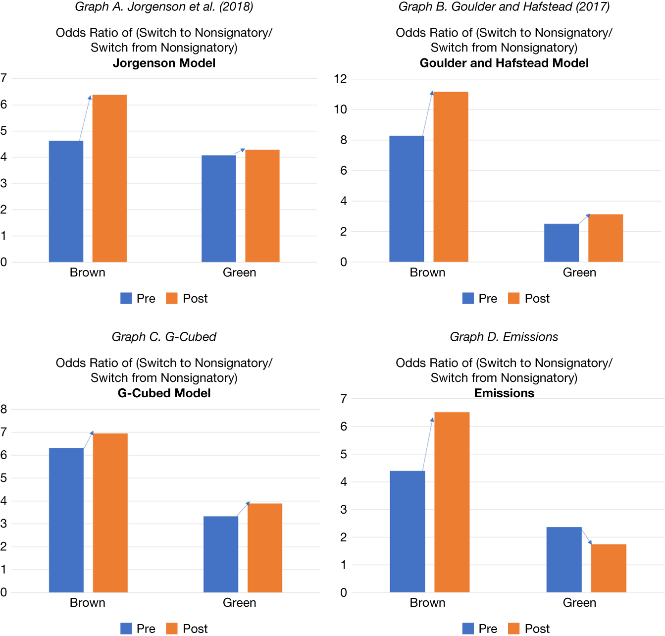
Figure 7 reports the odds ratios. Graph A, which is based on the Jorgenson et al. (Reference Jorgenson, Goettle, Ho and Wilcoxen2018) model, shows that the odds ratio of the most brown industries increased (from 4.6 to 6.4) after the signing of the Alliance. The odds ratio of the most green industries increased, but by relatively less (from 4.1 to 4.3) after signing the Alliance. Graphs B–D, which are based on Goulder and Hafstead (Reference Goulder and Hafstead2017), Bertram et al. (Reference Bertram, Boirard, Edmonds, Fernando, Gayle, Hurst, Liu, McKibbin, Payerols, Richters and Schets2022), and emission funding, respectively, show similar results.Footnote 38 This evidence indicates that relative to the most green industries, bank–borrower relationships moved from signatory to nonsignatory for the most brown industries.
Figure 7 shows the change in odds ratios of likelihood of switching to signatory lenders after the Net-Zero Banking Alliance for brown borrowers relative to green borrowers, where brown and green are classified based on various model scenarios. Graph A shows results from Jorgenson et al (Reference Jorgenson, Goettle, Ho and Wilcoxen2018), Graph B shows results from Goulder and Hafstead (Reference Goulder and Hafstead2017), Graph C shows results from Bertram et al. (Reference Bertram, Boirard, Edmonds, Fernando, Gayle, Hurst, Liu, McKibbin, Payerols, Richters and Schets2022), and Graph D shows results using carbon emissions. The odds ratio is calculated as the portion of borrowers who switched from a nonsignatory to a signatory, scaled by the portion of borrowers who switched from a signatory to a nonsignatory.

FIGURE 7 Long description
A four-panel set of bar charts labeled Graph A through D. Each graph shares a common Y-axis representing the Odds Ratio of Switch to Nonsignatory forward slash Switch from Nonsignatory and an X-axis with two categories: Brown and Green. Each category has two bars: blue for Pre and orange for Post. Blue arrows point from the top of the Pre bar to the top of the Post bar to indicate the direction of change.
* Graph A. Jorgenson et al. 2018: For Brown borrowers, the ratio increases from approximately 4.6 to 6.4. For Green borrowers, it increases slightly from 4.1 to 4.3.
* Graph B. Goulder and Hafstead 2018: For Brown borrowers, the ratio increases from 8.3 to 11.2. For Green borrowers, it increases from 2.5 to 3.1.
* Graph C. G-Cubed Model: For Brown borrowers, the ratio increases from 6.3 to 6.9. For Green borrowers, it increases from 3.3 to 3.9.
* Graph D. Emissions: For Brown borrowers, the ratio increases from 4.4 to 6.5. For Green borrowers, the ratio decreases from 2.4 to 1.7.
Table B.14 in the Supplementary Material shows consistent results based on a similar exercise comparing borrowing from highly exposed and less-exposed banks around the Paris Agreement. Together with our previous findings on lending volume, these results on borrowers’ switches show some evidence of banks’ responses, although limited to a reduction in their exposures to brown industries.
In sum, the evidence on banks’ responses to the Paris Agreement and the signing of the Net Zero Alliance offers some, arguably mixed, support for the static balance sheet assumption we made in our estimates of banks’ exposures to transition risk. However, the fact that banks’ responses were largely limited to a reduction in exposures to brown industries suggests that our bank exposure estimates can be viewed as an upper bound of banks’ exposures to transition risks.
V. Conclusion
There is growing interest in assessing the impact of transition risks on financial stability. However, most previous studies proxy transition risks using carbon emissions. In this article, we take a different approach. We combine loan-level data with GE sectoral estimates of changes in the U.S. economy following different transition policy scenarios. In contrast to carbon emissions, which are backward-looking, our estimates are forward-looking, and because they are computed from GE models, they capture a wider range of effects induced by policies to promote the transition to a low-carbon economy.
Our results show that banks’ exposures to transition risks are at their highest, 14% of their loan portfolios under the most severe scenario; however, they are about 0.5%–2% when accounting for historical loans’ PDs and LGDs. We estimate that exposures are up to 5 percentage points higher if the transition policy is implemented at the time of an economic downturn, with a relatively smaller effect if the policy coincides with a sectoral shock. Our results also show that a commonly used metric, past carbon emissions, is unable to explain at least 40% of the bank exposures estimated from GE models. Finally, while we find some evidence that U.S. banks are managing their exposures to transition risks, this effect is primarily driven by reduced lending to brown borrowers.
Our article suggests several fruitful areas for future research in the nexus between financial stability and climate change risks. For example, it would be useful to expand the analysis to asset managers and insurance companies given they retain substantial exposures to the same set of borrowers we considered. Given that we focused on transition risks, it would be worthwhile to expand our analysis to include physical risks. Finally, as we develop a better understanding of borrowers’ exposures to climate risks, it would be worthwhile to investigate how this exposure affects borrowers’ ability to access funding going forward.
Supplementary Material
To view supplementary material for this article, please visit http://doi.org/10.1017/S0022109026103226.