



1 Introduction
Consider a closed Riemannian manifold
 $(M,g)$
. When M has negative sectional curvature everywhere, the geodesic flow defined on the unit tangent bundle
 $SM$
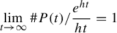
is a prime example of Anosov flow (cf. [Reference Anosov2], [Reference Katok and Hasselblatt25, §17.6]). There is correspondence between closed geodesics on M and periodic orbits under the geodesic flow, and they are important from both geometric and dynamical points of view. The asymptotic growth of the number of closed geodesics is given by the celebrated theorem of Margulis in his 1969 thesis [Reference Margulis34, Reference Margulis35] (the notation
 $f_1\sim f_2$
means that
 $\lim _{t\to \infty }({f_1(t)}/{f_2(t)})=1$
),
 $$ \begin{align} \begin{aligned} \#P(t)\sim\frac{e^{ht}}{ht}, \end{aligned} \end{align} $$
where
 $P(t)$
is the set of closed geodesics with length at most t and h is the topological entropy of the geodesic flow.
If M has non-positive curvature or has no focal/conjugate points, a free-homotopy class may have infinitely many closed geodesics. So we let
 $P(t)$
be the set of free-homotopy classes containing a closed geodesic on M with length at most t. Recently, Ricks [Reference Ricks47] established (1) for rank-one locally CAT
 $(0)$
spaces, which include rank-one manifolds with non-positive curvature. Climenhaga, Knieper, and War [Reference Climenhaga, Knieper and War14] proved (1) for a class of manifolds without conjugate points admitting background metrics of negative curvature. This class includes all compact surfaces of genus at least two. The problem remains widely open for general manifolds without conjugate points in higher dimension. Since it is interesting to consider higher dimensional manifolds allowing some positive curvature, the class of rank-one manifolds without focal points is an appropriate object of study.
1.1 Statement of main results
In this paper, we obtain Margulis-type asymptotic estimates (1) for all rank-one manifolds without focal points.
Theorem A. Let M be a rank-one closed Riemannian manifold without focal points, then
 $$ \begin{align*}\#P(t)\sim\frac{e^{ht}}{ht},\end{align*} $$
where h denotes the topological entropy of the geodesic flow on
 $SM$
.
Theorem A applies to all rank-one closed Riemannian manifolds without focal points, and hence all rank-one closed manifolds with non-positive curvature. In particular, it applies to Gromov’s graph manifolds of non-positive curvature (cf. [Reference Knieper27, p. 313]), which is not covered by the result of [Reference Climenhaga, Knieper and War14], see [Reference Climenhaga, Knieper and War13, Remark 2.1] for discussions. In fact, we can further modify Gromov’s graph manifolds a little bit as follows. We still start with a surface of constant negative curvature with one infinite cusp. Now, replace a small disk away from the cusp on this surface by a small cap, so that there is some positive sectional curvature but still no focal points on this surface. Continuing exactly as in the construction of Gromov’s graph manifolds, we get a rank-one manifold without focal points. Since this manifold has some positive sectional curvature, it is not covered by [Reference Ricks47]. However, there is a flat torus isometrically embedded in the middle portion of the manifold, so its fundamental group contains a free abelian subgroup of rank two. Then, the manifold cannot admit a metric of negative curvature and hence, the result of [Reference Climenhaga, Knieper and War14] does not apply.
In the proof of Theorem A, there are substantial technical difficulties compared with [Reference Climenhaga, Knieper and War14, Reference Ricks47]. Compared with rank-one locally CAT
 $(0)$
spaces or manifolds of non-positive curvature in [Reference Ricks47], the lack of convexity properties causes some difficulties, and some rigidity and comparison results do not hold any more, see Remarks 2.4, 3.6, and 3.8 below. We will conduct a careful study of the angle metric on the boundary at infinity of the universal cover. Using the angle metric instead of Tits metric, we establish a version of weak
 $\pi $
-convergence theorem, which plays a central role in establishing a closing lemma. We also adopt the new ideas in [Reference Climenhaga, Knieper and War14]: for example, the slice instead of full box is used in the intersection
 $S\cap \phi ^{-t} \gamma B$
(
 $\phi ^t$
denotes the geodesic flow, see §2.5 for notation), so there is no need to compute the average depth of intersection components as in [Reference Ricks47, §5.2].
Our setting also has significant difference from that in [Reference Climenhaga, Knieper and War14]. For example, manifolds without focal points do not have uniform visibility property in general, and thus, we have to develop weak
 $\pi $
-convergence theorem to prove a type of closing lemma. Moreover, in [Reference Climenhaga, Knieper and War14], by the Morse lemma, the
 $\Gamma $
-action (induced by deck transformations) on the boundary at infinity is topologically conjugate to the
 $\Gamma $
-action under the metric of negative curvature [Reference Climenhaga, Knieper and War14, Remark 2.6]. In our setting, the action has no such property and its behavior will be analyzed using the properties of no focal points. Moreover, instead of expansive vectors in [Reference Climenhaga, Knieper and War14], we use regular vectors as the centers of flow boxes. This simplifies our argument, especially Lemma 5.2.
We also obtain the following result of equidistribution of periodic orbits with respect to the Knieper measure. Recall that a
 $\phi $
-invariant probability measure
 $\mu $
is called the measure of maximal entropy (MME for short) if
 $h_{\mu }(\phi )\geq h_{\nu }(\phi )$
for any
 $\phi $
-invariant probability measure
 $\nu $
. By the variational principle,
 $h_{\mu }(\phi )=h$
. It is shown in [Reference Liu, Liu and Wang32] that MME is unique and can be constructed via Patterson–Sullivan measures. The unique MME is called the Knieper measure (see §2.4 for more details).
Theorem B. Suppose that M is a rank-one closed Riemannian manifold without focal points and
 $\epsilon \in (0, {\mathrm {inj}} (M)/2)$
is fixed, where
 ${\mathrm {inj}} (M)$
is the injectivity radius of M. For
 $t> 0$
, let
 $C(t)$
be any maximal set of pairwise non-free-homotopic closed geodesics with lengths in
 $(t-\epsilon , t]$
, and define the measure
 $$ \begin{align*}\nu_t:=\frac{1}{\# C(t)}\sum_{c\in C(t)}\frac{\mathrm{Leb}_c}{t},\end{align*} $$
where
 $\mathrm {Leb}_c$
is the Lebesgue measure along the curve
 $\dot c$
in the unit tangent bundle
 $SM$
.
Then, the measures
 $\nu _t$
converge in the weak
 $^*$
topology to the unique measure of maximal entropy as
 $t\to \infty $
.
In the last section, we show that the Knieper measure has the Bernoulli property, which is the strongest mixing property for measurable dynamical systems. We shall recall the necessary definitions of Kolmogorov/Bernoulli properties and known results from the literature.
Theorem C. Let M be a rank-one closed Riemannian manifold without focal points, then the unique measure of maximal entropy is Bernoulli.
1.2 Some history of Margulis’ asymptotic formula
The main ingredient in the proof of Margulis’ asymptotic formula (1) is from ergodic theory. Margulis [Reference Margulis35] constructed a measure which is invariant under the geodesic flow. This measure is mixing and the conditional measures on stable/unstable manifolds contract/expand with a uniform rate under the flow. Using different methods, Bowen constructed a measure of maximal entropy (MME for short) in [Reference Bowen5] for Axiom A flows. Later, in [Reference Bowen6], Bowen proved that MME is unique. It turns out that the measures constructed by Bowen and Margulis are eventually the same, and is called the Bowen–Margulis measure. The Bowen–Margulis measure has the Bernoulli property (cf. [Reference Ratner46]).
An alternative approach to (1) for Axiom A flows was given by Parry and Pollicott [Reference Parry and Pollicott40], based on zeta functions and symbolic dynamics. See the survey by Sharp in [Reference Margulis35] for further progress that has been made since Margulis’ thesis.
In 1984, A. Katok [Reference Burns and Katok8] conjectured that the geodesic flow on a closed rank-one manifold of non-positive curvature admits a unique MME. On such manifolds, the geodesic flow exhibits non-uniformly hyperbolic behavior. In 1998, Katok’s conjecture was finally settled by Knieper [Reference Knieper27]. In his proof, Knieper used Patterson–Sullivan measures on the boundary at infinity of the universal cover of M to construct an MME (called Knieper measure), and showed that this measure is the unique MME. Recently, Burns, Fisher, Climenhaga, and Thompson [Reference Burns, Climenhaga, Fisher and Thompson7] proved the uniqueness of equilibrium states for certain potentials, which generalized Knieper’s result.
Knieper’s measure can be used to obtain the following asymptotic estimates [Reference Knieper26, Reference Knieper28]: there exists
 $C>0$
such that for t large enough,
 $$ \begin{align*}\frac{1}{C}\frac{e^{ht}}{t}\le \#P(t)\le C \frac{e^{ht}}{t}.\end{align*} $$
Since then, efforts are made to improve the above to the Margulis-type asymptotic estimates (1). A preprint [Reference Gunesch24], though not published, contains many inspiring ideas to this problem. A breakthrough was made recently by Ricks [Reference Ricks47]: (1) is established for rank-one locally CAT
 $(0)$
spaces, which include rank-one manifolds with non-positive curvature.
Beyond non-positive curvature, manifolds without focal/conjugate points are studied extensively. Following Knieper’s method, Liu, Wang, and the author constructed the Knieper measure for rank-one manifolds without focal points and showed it is the unique MME [Reference Liu, Wang and Wu33]. Gelfert and Ruggiero [Reference Gelfert and Ruggiero23] also proved the uniqueness of MME for rank-one surfaces without focal points by different methods. Extending the approach in [Reference Burns, Climenhaga, Fisher and Thompson7], Chen, Kao, and Park proved the uniqueness of equilibrium states for certain potentials in [Reference Chen, Kao and Park10, Reference Chen, Kao and Park11]. Manifolds without conjugate points in general are far from being well understood. Remarkable progress was made by Climenhaga, Knieper, and War for a class of manifolds (including all surfaces with genus at least two) without conjugate points: the uniqueness of MME is proved in [Reference Climenhaga, Knieper and War13] and (1) is obtained in [Reference Climenhaga, Knieper and War14]. Weaver [Reference Weaver53] also obtained (1) for surfaces having negative curvature outside of a collection of radially symmetric caps.
In the non-positive curvature case, the Knieper measure is proved to be mixing in [Reference Babillot3] and Bernoulli in [Reference Call and Thompson9]. For rank-one manifolds without focal points, the Knieper measure is known to be mixing by [Reference Liu, Liu and Wang32] and have the Kolmogorov property by [Reference Chen, Kao and Park11]. The method of Call and Thompson [Reference Call and Thompson9] actually proves the Kolmogorov property of the unique equilibrium states for certain potentials [Reference Call and Thompson9, Reference Chen, Kao and Park11]. For the Knieper measure, to improve the Kolmogorov property to the Bernoulli property, we adapt the classical argument in [Reference Ornstein and Weiss37, Reference Ratner46] for Anosov flows. In fact, we follow closely [Reference Chernov and Haskell12], which is for systems with non-uniformly hyperbolic structure.
1.3 Organization of the paper
In §2, we recall some geometric and ergodic background on rank-one manifolds without foal points, including Busemann functions, construction of the Knieper measure, and local product flow boxes. Sections 3–6 are devoted to proving Theorem A. Meanwhile, Theorem B is proved in §6. In the last section, we prove Theorem C, that is, the Knieper measure for rank-one manifolds without focal points has the Bernoulli property.
2 Geometric and ergodic background
In this section, we present some geometric and ergodic results on rank-one manifolds without focal points, which will be used in the following discussions.
2.1 Rank-one manifolds without focal points
Suppose that
 $(M,g)$
is a
 $C^{\infty }$
closed n-dimensional Riemannian manifold, where g is a Riemannian metric. Let
 $\pi : SM\to M$
be the unit tangent bundle over M. For each
 $v\in S_pM$
, we always denote by
 $c_{v}: {\mathbb R}\to M$
the unique geodesic on M satisfying the initial conditions
 $c_v(0)=p$
and
 $\dot c_v(0)=v$
. The geodesic flow
 $\phi =(\phi ^{t})_{t\in \mathbb {R}}$
(generated by the Riemannian metric g) on
 $SM$
is defined as
 $$ \begin{align*} \phi^{t}: SM \rightarrow SM, \quad (p,v) \mapsto (c_{v}(t),\dot c_{v}(t))\quad \text{for all } t\in {\mathbb R}. \end{align*} $$
A vector field
 $J(t)$
along a geodesic
 $c:{\mathbb R}\to M$
is called a Jacobi field if it satisfies the Jacobi equation:
 $$ \begin{align*}J"+R(J, \dot c)\dot c=0,\end{align*} $$
where R is the Riemannian curvature tensor and
 $'$
denotes the covariant derivative along c.
Definition 2.1. Let c be a geodesic on
 $(M,g)$
.
-
(1) A pair of distinct points
 $p=c(t_{1})$
and
$q=c(t_{2})$
is called focal if there is a Jacobi field J along c such that
$J(t_{1})=0$
,
$J'(t_{1})\neq 0$
, and
${d}/{dt}\| J(t)\|^{2}\mid _{t=t_{2}}=0$
;
-
(2)
$p=c(t_{1})$
and
$q=c(t_{2})$
are called conjugate if there is a non-trivial Jacobi field J along c such that
$J(t_{1})=0=J(t_{2})$
.


A compact Riemannian manifold
 $(M,g)$
is called a manifold without focal/conjugate points if there is no focal/conjugate points on any geodesic in
 $(M,g)$
.
By definition, if a manifold has no focal points, then it has no conjugate points. All manifolds of non-positive curvature always have no focal points.
A Jacobi field
 $J(t)$
along a geodesic
 $c(t)$
is called parallel if
 $J'(t)=0$
for all
 $t\in {\mathbb R}$
. The notion of rank is defined as follows.
Definition 2.2. For each
 $v \in SM$
, we define rank(v) to be the dimension of the vector space of parallel Jacobi fields along the geodesic
 $c_{v}$
, and rank(M):=
 $\min \{$
rank
 $(v): v \in SM\}$
. For a geodesic c, we define rank(c)=rank(
 $\dot c(t)$
)
 $\text { for all }\ t\in \mathbb {R}$
.
Let M be a rank-one closed Riemannian manifold without focal points. Then,
 $SM$
splits into two subsets invariant under the geodesic flow: the regular set
 $\text {Reg}:= \{v\in SM: \text {rank}(v)=1\}$
and the singular set
 $\text {Sing}:= SM \setminus \text {Reg}$
.
2.2 Geometric properties and boundary at infinity
Let M be a closed Riemannian manifold without focal points and
 ${\text {pr}}: X\to M$
the universal cover of M. Let
 $\Gamma \simeq \pi _1(M)$
be the group of deck transformations on X so that each
 $\gamma \in \Gamma $
acts isometrically on X. Since
 $M=X/\Gamma $
is compact, each
 $\gamma \in \Gamma $
is axial (cf. [Reference Croke and Schroeder16, Lemma 2.1]), that is, there exists a geodesic c and
 $t_{0}>0$
such that
 $\gamma (c(t)) = c(t+t_{0})$
for every
 $t\in \mathbb {R}$
. Correspondingly, c is called an axis of
 $\gamma $
and we denote
 $|\gamma |:=t_0$
, where
 $t_0$
is minimal with the above property.
We still denote by
 ${\text {pr}}: SX\to SM$
and
 $\gamma : SX\to SX$
the maps on unit tangent bundles induced by
 ${\text {pr}}$
and
 $\gamma \in \Gamma $
. From now on, we use an underline to denote objects in M and
 $SM$
, e.g. for a geodesic c in X and
 $v\in SX$
,
 ${\underline c}:={\text {pr}} c$
,
 ${\underline v}:={\text {pr}} v$
denote their projections to M and
 $SM$
, respectively. Denote by d both the distance functions on M and X induced by Riemannian metrics. The Sasaki metrics on
 $SM$
and
 $SX$
are also denoted by d if there is no confusion.
Suppose that
 $c_{1}$
and
 $c_{2}$
are both geodesics in X. We call that
 $c_{1}$
and
 $c_{2}$
are positively asymptotic or just asymptotic if there is a positive number
 $C> 0$
such that
 $$ \begin{align} d(c_{1}(t),c_{2}(t)) \leq C \quad\text{for all } t \geq 0. \end{align} $$
We say
 $c_{1}$
and
 $c_{2}$
are negatively asymptotic if (2) holds for all
 $t \leq 0$
. Here,
 $c_{1}$
and
 $c_{2}$
are said to be bi-asymptotic or parallel if they are both positively and negatively asymptotic. The relation of positive/negative asymptoticity is an equivalence relation between geodesics on X. The class of geodesics that are positively/negatively asymptotic to a given geodesic
 $c_v$
is denoted by
 $c_v(+\infty )$
/
 $c_v(-\infty )$
or
 $v^+/v^-$
, respectively. We call them points at infinity. Obviously,
 $c_{v}(-\infty )=c_{-v}(+\infty )$
. We use
 ${\partial X}$
to denote the set of all points at infinity and call it the boundary at infinity, or the ideal boundary. If
 $\eta =v^+\in {\partial X}$
, we say that v points at
 $\eta .$
The following are the fundamental properties of the geometry of manifolds without focal points.
Lemma 2.3. (Cf. [Reference O’Sullivan36])
Let X be a simply connected closed Riemannian manifold without focal points.
-
(1) Let
$c_1$
and
$c_2$
be distinct geodesics with
$c_1(0)=c_2(0)$
. Then, for
$t>0$
, both
$d(c_1(t), c_2)$
and
$d(c_1(t), c_2(t))$
are strictly increasing and tend to infinity as
$t\to \infty $
. -
(2) Let
$c_1$
and
$c_2$
be asymptotic geodesics. Then, both
$d(c_1(t), c_2)$
and
$d(c_1(t), c_2(t))$
are non-increasing functions of
$t\in {\mathbb R}$
. -
(3) For any geodesic c and each
$p\in X$
, there exists a unique geodesic through p and asymptotic to c. -
(4) (Flat strip lemma) If
$c_1$
and
$c_2$
are bi-asymptotic, then they bound a flat strip, that is, there is an isometric embedding
$\varphi : [0,a]\times {\mathbb R}\to X$
such that
$\varphi (0,t)=c_1(t)$
and
$\varphi (a,t)=c_2(t)$
up to parameterization.


Remark 2.4. If X has non-positive curvature, for any two geodesics
 $c_1$
and
 $c_2$
, both the functions
 $d(c_1(t), c_2)$
and
 $d(c_1(t), c_2(t))$
are convex in
 $t\in {\mathbb R}$
. This is not true for general manifolds without focal points. The lack of convexity causes difficulties in many problems for manifolds without focal points.
We can define the visual topology on
 ${\partial X}$
following [Reference Eberlein19, Reference Eberlein and O’Neill20]. For each p, by Lemma 2.3, there is a bijection
 $f_p: S_pX\to {\partial X}$
defined by
 $f_p(v)=v^+, v\in S_pX$
. So for each
 ${p\in M}$
,
 $f_p$
induces a topology on
 ${\partial X}$
from the usual topology on
 $S_pX$
. Given
 $p,q\in X$
, let
 $\psi : S_pX\to S_qX$
be the map such that
 $\psi (v)$
is the unique vector in
 $S_qX$
asymptotic to
 ${v\in S_pX}$
.
Lemma 2.5. [Reference Watkins52, Lemma 2.6]
The map
 $\psi : S_pX\to S_qX$
above is continuous.
It follows that
 $\psi $
is in fact a homeomorphism. Hence, the topology on
 ${\partial X}$
induced by
 $f_p$
is independent of
 $p\in X$
and is called the visual topology on
 ${\partial X}$
.
The above topology on
 ${\partial X}$
and the manifold topology on X can be extended to
 ${\overline X:= X\cup {\partial X}}$
naturally by requiring the map
 $\varphi $
defined as follows is a homeomorphism. Fix
 $p\in X$
. For each
 $v\in T_pX$
with
 $\|v\|\le 1$
, define
 $$ \begin{align*} \varphi(v):=\begin{cases}\exp \bigg(\dfrac{v}{1-\|v\|}\bigg) & \text{if } |v\|<1, \\ f_p(v) &\text{if } |v\|=1. \end{cases} \end{align*} $$
This topology is usually called the cone topology. Under this topology,
 $\overline {X}$
is homeomorphic to the closed unit ball in
 $\mathbb {R}^{\text {dim}(X)}$
and
 ${\partial X}$
is homeomorphic to the unit sphere
 $\mathbb {S}^{\text {dim}(X)-1}$
.
The following continuity property is useful.
Lemma 2.6. [Reference Watkins52, Lemma 6.4]
Let
 $p, p_n\in X$
with
 $p_n\to p$
, and
 $x_n,\zeta \in \overline X$
with
 ${x_n\to \zeta }$
. Then,
 $\dot c_{p_nx_n}(0)\to \dot c_{p\zeta }(0)$
, where
 $c_{qx}$
is the unique geodesic starting from
 $q\in X$
and pointing at
 $x\in \overline X$
.
2.3 Continuity of Busemann function
For each pair of points
 $(p,q)\in X \times X$
and each point at infinity
 $\xi \in {\partial X}$
, the Busemann function based at
 $\xi $
and normalized by p is
 $$ \begin{align*}b_{\xi}(q,p):=\lim_{t\rightarrow +\infty}(d(q,c_{p,\xi}(t))-t),\end{align*} $$
where
 $c_{p,\xi }$
is the unique geodesic starting from p and pointing at
 $\xi $
. The Busemann function
 $b_{\xi }(q,p)$
is well defined since the function
 $t \mapsto d(q,c_{p,\xi }(t))-t$
is bounded from above by
 $d(p,q)$
and decreasing in t (this can be checked by using the triangle inequality). If
 $v\in S_pX$
points at
 $\xi \in {\partial X}$
, we also write
 $b_v(q):=b_{\xi }(q,p).$
The level sets of the Busemann function
 $b_{\xi }(\cdot ,p)$
are called the horospheres centered at
 $\xi $
. The horosphere through p based at
 $\xi \in {\partial X}$
is denoted by
 $H_p(\xi )$
. For more details of the Busemann functions and horospheres, please see [Reference Dal’Bo, Peigné and Sambusetti17, Reference Ruggiero48, Reference Ruggiero49]. Here, we are concerned with the continuity property of the horospheres and Busemann functions.
We say that the manifold M satisfies the axiom of asymptoticity if for every
 $v\in SX$
, the following statement holds. For any choice of
 $x_n, x\in X, v_n\in SX$
,
 $x_n\to x$
,
 $v_n\to v$
and a sequence of numbers
 $t_n\to \infty $
, the sequence
 $c_n$
of geodesic segments joining
 $x_n$
to
 $c_{v_n}(t_n)$
converges to an asymptote of
 $c_v$
.
Proposition 2.7. (Cf. [Reference Pesin43, Theorem 6.1] [Reference Ruggiero48, Lemma 1.2])
Let M be a closed Riemannian manifold without conjugate points that satisfies the the axiom of asymptoticity. Then, for every
 $p\in X$
, the map
 $\xi \mapsto H_\xi (p)$
is continuous in the following sense: if
 $\xi _n\to \xi \in {\partial X}$
and
 $K\subset X$
is compact, then
 $H_{\xi _n}(p)\cap K\to H_\xi (p)\cap K$
uniformly in the Hausdorff topology.
Proposition 2.8. (Cf. [Reference Pesin43, Theorem 5.2])
If the manifold M has no focal points, then it satisfies the the axiom of asymptoticity.
By Proposition 2.8, Proposition 2.7 applies to manifolds without focal points. So we have the following corollary (see also [Reference Liu, Wang and Wu33, Proposition 9]).
Corollary 2.9. The functions
 $(v,q)\mapsto b_v(q)$
and
 $(\xi ,p,q)\mapsto b_\xi (p,q)$
are continuous on
 $SX\times X$
and
 ${\partial X}\times X\times X$
, respectively.
We would like to obtain a certain equicontinuity of the Busemann function
 $v\mapsto b_v(q)$
. The idea is to extend the function to the compact space
 $X\cup {\partial X}$
. Given
 $x,p,q\in X$
, define
 $$ \begin{align*}b_x(q,p):=d(q,x)-d(p,x).\end{align*} $$
Lemma 2.10. [Reference Liu, Wang and Wu33, Proposition 10]
For each pair of points
 $p,q\in X$
, if there is a sequence
 $\{x_{n}\}\subset X$
with
 $\lim _{n\rightarrow +\infty }x_{n}=\xi \in {\partial X}$
, then
 $$ \begin{align*}\lim_{n\rightarrow +\infty}b_{x_n}(q,p)=b_{\xi}(q,p).\end{align*} $$
For any
 $p\in X, v,w\in S_pX$
, denote by
 $\angle _p(v,w)$
the angle at p between v and w which is no more than
 $\pi $
.
Lemma 2.11. Let
 $p{\kern-1pt}\in{\kern-1pt} X$
,
 $A{\kern-1pt}\subset{\kern-1pt} S_pX$
be closed, and
 $B{\kern-1pt}\subset{\kern-1pt} X$
be such that
 ${A^+:= \{v^+: v\in A\}}$
and
 $B^\infty := \{\lim _n q_n \in {\partial X}: q_n\in B\}$
are disjoint subsets of
 ${\partial X}$
. Then, the family of functions
 $A\to {\mathbb R}$
indexed by B and given by
 $v\mapsto b_v(q)$
are equicontinuous: for every
 $\epsilon>0$
, there exists
 $\delta>0$
such that if
 $\angle _p(v,w)<\delta $
, then
 $|b_v(q)-b_w(q)|<\epsilon $
for every
 $q\in B$
.
Proof. The proof is a repetition of that of [Reference Climenhaga, Knieper and War14, Lemma A.1] and is thus omitted. Notice that in our setting, Lemma 2.10 should be used instead of [Reference Climenhaga, Knieper and War13, Corollary 2.18].
2.4 Patterson–Sullivan measure and Knieper measure
We recall the construction of the Patterson–Sullivan measure and Knieper measure in this section. Let us start with the definition of Busemann density.
Definition 2.12. Let X be a simply connected rank-one manifold without focal points and
 $\Gamma $
a discrete subgroup of
 $\text {Iso}(X)$
, the group of isometries of X. For a given constant
 $r>0$
, a family of finite Borel measures
 $\{\mu _{p}\}_{p\in X}$
on
 ${\partial X}$
is called an r-dimensional Busemann density if:
-
(1) for any
$p,\ q \in X$
and
$\mu _{p}$
-almost every (a.e.)
$\xi \in {\partial X}$
, where
$$ \begin{align*}\frac{d\mu_{q}}{d \mu_{p}}(\xi)=e^{-r \cdot b_{\xi}(q,p)},\end{align*} $$
$b_{\xi }(q,p)$
is the Busemann function;
-
(2)
$\{\mu _{p}\}_{p\in X}$
is
$\Gamma $
-equivariant, that is, for all Borel sets
$A \subset {\partial X}$
and for any
$\gamma \in \Gamma $
, we have
$$ \begin{align*}\mu_{\gamma p}(\gamma A) = \mu_{p}(A).\end{align*} $$


The construction of such a Busemann density is due to Patterson [Reference Patterson41] in the case of Fuchsian groups and generalized by Sullivan [Reference Sullivan50] for hyperbolic spaces.
Extending the techniques in [Reference Knieper27] to rank-one manifolds without focal points, we constructed Busemann density via Patterson–Sullivan construction and showed the following theorem in [Reference Liu, Wang and Wu33].
Theorem 2.13. [Reference Liu, Wang and Wu33, Theorem B]
Let
 $M=X/\Gamma $
be a compact rank-one manifold without focal points. Then, up to a multiplicative constant, the Busemann density is unique, that is, the Patterson–Sullivan measure is the unique Busemann density.
Let
 $\{\mu _{p}\}_{p\in X}$
be the Patterson–Sullivan measure, which is the unique Busemann density with dimension h. Let
 $P:SX \to {\partial X} \times {\partial X}$
be the projection given by
 $P(v)=(v^-,v^+)$
. Denote by
 $\mathcal {I}^{P}:=P(SX)=\{P(v): v \in SX\}$
the subset of pairs in
 ${\partial X} \times {\partial X}$
that can be connected by a geodesic. Note that the connecting geodesic may not be unique and, moreover, not every pair
 $\xi \neq \eta $
in
 ${\partial X}$
can be connected by a geodesic.
Fix a point
 $p\in X$
. We can define a
 $\Gamma $
-invariant measure
 $\overline {\mu }$
on
 $\mathcal {I}^{P}$
by the following formula:
 $$ \begin{align} d \overline{\mu}(\xi,\eta) := e^{h\cdot \beta_{p}(\xi,\eta)}d\mu_{p}(\xi) d\mu_{p}(\eta), \end{align} $$
where
 $\beta _{p}(\xi ,\eta ):=-\{b_{\xi }(q, p)+b_{\eta }(q, p)\}$
is the Gromov product, and q is any point on a geodesic c connecting
 $\xi $
and
 $\eta $
. It is easy to see that the function
 $\beta _{p}(\xi ,\eta )$
does not depend on the choice of c and q. In geometric language, the Gromov product
 $\beta _{p}(\xi ,\eta )$
is the length of the part of a geodesic c between the horospheres
 $H_{\xi }(p)$
and
 $H_{\eta }(p)$
.
Then,
 $\overline {\mu }$
induces a
 $\phi $
-invariant measure m on
 $SX$
with
 $$ \begin{align} m(A):=\int_{\mathcal{I}^{P}} \text{Vol} \{\pi(P^{-1}(\xi,\eta)\cap A)\}\,d \overline{\mu}(\xi,\eta) \end{align} $$
for all Borel sets
 $A\subset SX$
. Here,
 $\pi : SX \rightarrow X$
is the standard projection map and Vol is the induced volume form on
 $\pi (P^{-1}(\xi ,\eta ))$
. Indeed, if there are more than one geodesic connecting
 $\xi $
and
 $\eta $
, then by the flat strip theorem,
 $\pi (P^{-1}(\xi ,\eta ))$
is a flat submanifold in X.
For any Borel set
 $A\subset SX$
and
 $t\in \mathbb {R}$
,
 $\text {Vol}\{\pi (P^{-1}(\xi ,\eta )\cap \phi ^{t}A)\}= \text {Vol}\{\pi (P^{-1}(\xi ,\eta ) \cap A)\}$
. Therefore, m is
 $\phi $
-invariant. Moreover,
 $\Gamma $
-invariance of
 $\overline {\mu }$
leads to the
 $\Gamma $
-invariance of m. Thus, m induces a
 $\phi $
-invariant measure on
 $SM$
satisfying
 $$ \begin{align*} m(A)=\int_{SM} \#(\text{pr}^{-1}({\underline v})\cap A)\,d{\underline m}({\underline v}). \end{align*} $$
It is proved in [Reference Liu, Wang and Wu33] that
 ${\underline m}$
is the unique MME, which is called the Knieper measure. Furthermore,
 ${\underline m}$
is proved to be mixing in [Reference Liu, Liu and Wang32] and Kolmogorov in [Reference Chen, Kao and Park11]. In the last section, we prove that
 ${\underline m}$
is Bernoulli.
2.5 Local product flow boxes
From now on, we fix
 $v_0\in SX$
such that
 ${\underline v}_0:={\text {pr}} v_0$
is a periodic and regular vector in
 $SM$
. Let
 $p:=\pi (v_0)$
, which will be the reference point in the following discussions. For simplicity, we will suppress
 $v_0$
and p from the notation. We also fix a scale
 $\epsilon \in (0, \min \{\tfrac 18, {{\text {inj}} (M)}/{4}\})$
.
The Hopf map
 $H: SX\to {\partial X}\times {\partial X}\times {\mathbb R}$
for
 $p\in X$
is defined as
 $$ \begin{align*}H(v):=(v^-, v^+, s(v)) \quad\text{where } s(v):=b_{v^-}(\pi v, p).\end{align*} $$
From definition, we see
 $s(\phi ^t v)=s(v)+t$
for any
 $v\in SX$
and
 $t\in {\mathbb R}$
. Here, s is continuous by Corollary 2.9.
Following [Reference Climenhaga, Knieper and War14], we define for each
 $\theta>0$
and
 $0<\alpha <\tfrac 32\epsilon $
,
 $$ \begin{align*} &\textbf{P}=\textbf{P}_\theta:=\{w^-: w\in S_pX \text{ and } \angle_p(w, v_0)\le \theta\},\\&\textbf{F}=\textbf{F}_\theta:=\{w^+: w\in S_pX \text{ and } \angle_p(w, v_0)\le \theta\},\\&B=B_\theta^\alpha:=H^{-1}(\textbf{P}\times \textbf{F}\times [0,\alpha]),\\&S=S_\theta:=B_\theta^{\epsilon^2}=H^{-1}(\textbf{P}\times \textbf{F}\times [0,\epsilon^2]). \end{align*} $$
Here,
 $B=B_\theta ^\alpha $
is called a flow box with depth
 $\alpha $
and
 $S=S_\theta $
is a slice with depth
 $\epsilon ^2$
. We will consider
 $\theta>0$
small enough, which will be specified in the following.
The following lemma is a variation of [Reference Ricks47, Lemma 1], which was crucial in constructing the Knieper measure.
Proposition 2.14. [Reference Liu, Wang and Wu33, Propositions 6 and 7]
Let X be a simply connected rank-one manifold without focal points and
 $v_0\in SX$
is regular. Then, for any
 $\epsilon>0$
, there is a
 $\theta _1> 0$
such that, for any
 $\xi \in \textbf {P}_{\theta _1}$
and
 $\eta \in \textbf {F}_{\theta _1}$
, there is a unique geodesic
 $c_{\xi ,\eta }$
connecting
 $\xi $
and
 $\eta $
, that is,
 $c_{\xi ,\eta }(-\infty )=\xi $
and
 $c_{\xi ,\eta }(+\infty )=\eta $
.
Moreover, the geodesic
 $c_{\xi ,\eta }$
is regular and
 $d(c_{v}(0), c_{\xi ,\eta })<\epsilon /10$
.
Based on Proposition 2.14, we have the following result.
Lemma 2.15. Let
 $v_0, p, \epsilon $
be as above and
 $\theta _1$
be given in Proposition 2.14. Then, for any
 $0<\theta <\theta _1$
:
-
(1)
$\mathrm {diam\ } \pi H^{-1}(\textbf {P}\times \textbf {F}\times \{0\})<{\epsilon }/{2}$
; -
(2)
$H^{-1}(\textbf {P}\times \textbf {F}\times \{0\})\subset SX$
is compact; -
(3)
$B_\theta ^\alpha $
is compact; -
(4)
$\mathrm {diam\ } \pi B_\theta ^\alpha <4\epsilon $
for any
$0<\alpha \le {3\epsilon }/{2}$
.


Proof. Assume the contrary of item (1), that is, there exist
 $\theta _n\to 0$
,
 $v_n,w_n\in H^{-1}(\textbf {P}_{\theta _n}\times \textbf {F}_{\theta _n}\times \{0\})$
such that
 $d(\pi v_n,\pi w_n)\ge {\epsilon }/{2}$
.
By Proposition 2.14, for n large enough, we know that
 $d(p, c_{v_n})<{\epsilon }/{10}$
and
 $d(p, c_{w_n})<{\epsilon }/{10}$
. Let
 $v_n'=\phi ^{t_n}v_n$
and
 $w_n'=\phi ^{s_n}w_n$
be such that
 $\pi v^{\prime }_n$
and
 $\pi w^{\prime }_n$
are the projections of p onto
 $c_{v_n}$
and
 $c_{w_n}$
, respectively. So,
 $$ \begin{align*} \begin{aligned} |t_n|&=|b_{v_n^{-}}(\pi v_n',p)|\le d(\pi v_n',p)<\frac{\epsilon}{10},\\ |s_n|&=|b_{w_n^{-}}(\pi w_n',p)|\le d(\pi w_n',p)<\frac{\epsilon}{10}. \end{aligned} \end{align*} $$
By passing to a subsequence, we can assume that
 $v_n'\to v, w_n'\to w$
. Notice that as
 ${\theta _n\to 0}$
, we know that
 $v^+=w^+=(v_0)^+$
and
 $v^-=w^-=(v_0)^-$
. Thus, by Proposition 2.14,
 $v=\phi ^tv_0$
and
 $w=\phi ^sv_0$
for some
 $t,s\in {\mathbb R}$
with
 $0\le |s|,|t|\le {\epsilon }/{10}$
. So
 ${d(\pi v, \pi w)\le {\epsilon }/{5}}$
.
However, we know by the triangle inequality that
 $$ \begin{align*} \begin{aligned} d(\pi v,\pi w)&=\lim_{n\to \infty}d(\pi v^{\prime}_n,\pi w^{\prime}_n)\\ &\ge \lim_{n\to \infty}(d(\pi v_n,\pi w_n)-d(\pi v_n,\pi v^{\prime}_n)-d(\pi w_n,\pi w^{\prime}_n))\\ &\ge \lim_{n\to \infty}\bigg(\frac{\epsilon}{2}-|t_n|-|s_n|\bigg)\ge \frac{\epsilon}{2}-\frac{\epsilon}{10}-\frac{\epsilon}{10}>\frac{\epsilon}{5}. \end{aligned} \end{align*} $$
We arrive at a contradiction. So
 $\text {diam } \pi H^{-1}(\textbf {P}\times \textbf {F}\times \{0\})\le {\epsilon }/{2}$
.
By the continuity of H,
 $H^{-1}(\textbf {P}\times \textbf {F}\times \{0\})\subset SX$
is closed. As the diameter of its projection under
 $\pi $
is no more than
 ${\epsilon }/{2}$
, we know
 $H^{-1}(\textbf {P}\times \textbf {F}\times \{0\})\subset SX$
is bounded. Thus, it is compact. The fact that
 $B_\theta ^\alpha $
is compact can be proved similarly.
Finally, by the triangle inequality, for any
 $0<\alpha \le {\epsilon }/{2}$
, we have
 $\text {diam } \pi B_\theta ^\alpha <{\epsilon }/{2}+2\alpha <4\epsilon $
.
At last, we also assume that the choice of
 $\theta \in (0, \theta _1)$
satisfies the following properties. Since
 $\theta \mapsto \bar \mu (\textbf {P}_\theta \times \textbf {F}_\theta )$
is non-decreasing and hence has at most countably many discontinuities, we always choose
 $\theta $
to be the continuity point of this function, that is,
 $$ \begin{align*}\lim_{\rho\to \theta}\bar\mu(\textbf{P}_\rho\times \textbf{F}_\rho)=\bar\mu(\textbf{P}_\theta\times \textbf{F}_\theta).\end{align*} $$
Furthermore,
 $\theta $
is chosen so that
 $\bar \mu (\partial \textbf {P}_\theta \times \partial \textbf {F}_\theta )=0.$
By the product structure of B and S, and the definition of m, we have for any
 $\alpha \in (0,{3\epsilon }/{2})$
,
 $$ \begin{align} \begin{aligned} \lim_{\rho\to \theta} m(S_\rho)=m(S_\theta), \quad \lim_{\rho\to \theta} m(B^\alpha_\rho)=m(B^\alpha_\theta) \quad\text{and}\quad m(\partial B^\alpha_\theta)=0. \end{aligned} \end{align} $$
The following is a direct corollary of Lemma 2.11.
Corollary 2.16. Given
 $v_0, p, \epsilon>0$
as above, there exists
 $\theta _2>0$
such that for any
 $0<\theta <\theta _2$
, if
 $\xi ,\eta \in \textbf {P}_\theta $
and any q lying within
 $4\epsilon $
of
 $\pi H^{-1}(\textbf {P}_\theta \times \textbf {F}_\theta \times [0,\infty ))$
, we have
 $|b_\xi (q,p)-b_\eta (q,p)|<\epsilon ^2$
. A similar result holds if the roles of
 $\textbf {P}_\theta $
and
 $\textbf {F}_\theta $
are reversed.
Let
 $\theta _0:=\min \{\theta _1, \theta _2\}$
, where
 $\theta _1$
is given in Lemma 2.15 and
 $\theta _2$
is given in Corollary 2.16. In the following, we always suppose that
 $0<\theta <\theta _0$
and (5) is satisfied.
3 Closing lemma
The aim of this section is to establish a type of closing Lemma 3.11. We need to study the properties of angle metric and prove a weak
 $\pi $
-convergence Theorem 3.9.
3.1 Angle metric
The angle metric on
 $\partial X$
is defined as
 $$ \begin{align*}\angle(\xi,\eta):=\sup_{x\in X}\angle_x(\xi,\eta) \quad \text{for all } \xi, \eta\in {\partial X}.\end{align*} $$
Then, the angle metric defines a path metric
 $d_T$
on
 ${\partial X}$
, called the Tits metric. Clearly,
 $d_T\ge \angle $
. The angle metric induces a topology on
 $\partial X$
finer than the visual topology.
Since
 $\angle $
is a supremum of a continuous function, it is lower semicontinuous.
Lemma 3.1. (Cf. [Reference Watkins52, Proposition 2.7])
The angle metric is lower semicontinuous, that is, if
 $\xi _n\to \xi $
and
 $\eta _n\to \eta $
in the visual topology, then
 $$ \begin{align*}\angle(\xi,\eta)\leq \liminf_{n\to \infty}\angle(\xi_n,\eta_n).\end{align*} $$
Using Lemma 2.3 and the first variation formula, we get the following fact, see [Reference Druetta and Ferraris18, Lemma 1.1] for another proof.
Lemma 3.2. (Cf. [Reference Watkins52, Lemma 2.9] and [Reference Druetta and Ferraris18, Lemma 1.1])
Let
 $v\in SX$
point at
 $\xi \in {\partial X}$
and let
 $\eta \in {\partial X}$
. Then,
 $$ \begin{align*}t\mapsto \angle_{c_v(t)}(\xi,\eta)\end{align*} $$
is a non-decreasing function. Equivalently,
 $$ \begin{align*}\angle_{c_v(t_1)}(c(\infty),\eta)+\angle_{c_v(t_2)}(c(-\infty),\eta)\le \pi\end{align*} $$
for any
 $t_1<t_2$
.
Proposition 3.3. Let
 $v\in SX$
point at
 $\xi \in {\partial X}$
and let
 $\eta \in {\partial X}$
. Then,
 $$ \begin{align*}\angle(\xi,\eta)=\lim_{t\to\infty} \angle_{c_v(t)}(\xi,\eta).\end{align*} $$
Proof. The above limit exists by Lemma 3.2. Let
 $q\in X$
and
 $t_n\to \infty $
as
 $n\to \infty $
. Denote
 $v_n:=g^{t_n}v, p_n:=\pi v_n$
. Let
 $c_n$
be the unique geodesic from q to
 $p_n$
. Write
 ${v_n'=\dot c_n(d(q, p_n))}$
.
We claim that
 $\angle _{p_n}(v_n,v_n')\to 0$
. Assuming the claim, then by Lemmas 3.2 and 2.6,
 $$ \begin{align*} &\lim_{n\to \infty}\angle_{p_n}(\eta,v_n)=\lim_{n\to \infty}\angle_{p_n}(\eta,v^{\prime}_n)\\ &\quad\ge \lim_{n\to \infty}\angle_q(\eta, \dot c_n(0))=\angle_q(\eta, \xi). \end{align*} $$
Since q is arbitrary, the proposition follows.
It remains to prove the claim. Assume the contrary for contradiction, that is,
 $\angle _{p_n}(v_n,v_n')\ge \alpha $
for some
 $\alpha>0$
by passing to a subsequence. Fix a fundamental domain
 ${\mathcal {F}}\subset X$
containing
 $\pi v$
. Let
 $\gamma _n\in \Gamma $
be such that
 $\gamma _n p_n\in {\mathcal {F}}$
. Since
 $\overline {\mathcal {F}}$
is compact, by passing to a subsequence, we assume that
 $\gamma _n p_n\to p\in \overline {\mathcal {F}}$
. Define
 $\sigma _n$
to be the geodesic from
 $\gamma _np_n$
to
 $\gamma _n \pi v$
, and
 $\tau _n$
to be the geodesic from
 $\gamma _np_n$
to
 $\gamma _n q$
. Denote
 $s_n:=d(\gamma _np_n, \gamma _n q)$
and recall that
 $t_n=d(\gamma _np_n, \gamma _n \pi v)$
. By the triangle inequality,
 $|s_n-t_n|\le d(\gamma _n \pi v, \gamma _n q)=d(\pi v,q)$
. So
 $\lim _{n\to \infty }s_n=\infty $
. Without loss of generality, assume
 $s_n\le t_n$
. For any
 $0\le t\le s_n$
, by Lemma 2.3(1),
 $$ \begin{align*}d(\sigma_n(t), \tau_n(t))\le d(\sigma_n(s_n), \tau_n(s_n))\le 2d(\pi v,q).\end{align*} $$
Now, by passing to a subsequence, suppose that
 $\dot \sigma _n(0)\to \dot \sigma (0)$
and
 $\dot \tau _n(0)\to \dot \tau (0)$
. Then,
 $\sigma $
and
 $\tau $
are two geodesics starting from p with
 $\angle _p(\dot \sigma (0), \dot \tau (0))\ge \alpha>0$
and
 $d(\sigma (t), \tau (t))\le 2d(\pi v,q)$
for any
 $t>0$
, which is a contradiction to Lemma 2.3(1). This proves the claim and the proposition.
Remark 3.4. If
 $X/ \Gamma $
is not compact, the above proposition holds if
 $v\in SX$
is assumed to be recurrent (cf. [Reference Watkins52, Corollary 2.11]). Our proof above uses the compactness of
 $X/\Gamma $
and works for arbitrary
 $v\in SX$
.
The following lemma is a rigidity counterpart of Lemma 3.2. It is a fundamental difference from the non-positive curvature case that the geodesic considered in the lemma is required to be recurrent. We do not know if the recurrence assumption can be removed.
Lemma 3.5. [Reference Watkins52, Corollary 6.8]
Let c be a recurrent geodesic, and suppose there exists
 $\xi \in {\partial X}$
such that
 $\angle _{c(t)}(\xi , c(\infty ))=\theta $
for all t and some
 $0<\theta < \pi $
. Then, c is the boundary of a flat half-plane.
Remark 3.6. In the non-positive curvature case, there is a much easier proof of the above lemma (without the recurrence assumption) using the following rigidity fact: if
 $t_1<t_2$
and
 $$ \begin{align*}\angle_{c(t_1)}(\xi, c(\infty))+\angle_{c(t_2)}(\xi, c(-\infty))=\pi,\end{align*} $$
then the infinite triangle with vertices
 $c(t_1), c(t_2), \xi $
is flat. This rigidity fact does not hold for general manifolds without focal points.
The following proposition on the Tits metric will not be used in subsequent discussions, but may have independent interest.
Proposition 3.7. Let c be a recurrent geodesic, not the boundary of a flat half-plane. Then,
 $$ \begin{align*}d_T(c(-\infty),c(\infty))>\pi.\end{align*} $$
Proof. At first,
 $$ \begin{align*}d_T(c(-\infty),c(\infty))\ge \angle(c(-\infty),c(\infty))\ge \angle_{c(0)}(c(-\infty),c(\infty))=\pi.\end{align*} $$
Assume for contradiction that
 $d_T(c(-\infty ),c(\infty ))=\pi .$
Recall that
 $({\partial X}, d_T)$
is a length space. It follows that there exist points
 $\eta _i\in {\partial X}$
such that
 $\lim _{i\to \infty }d_T(\eta _i, c(-\infty ))={\pi }/{2}$
and
 $\lim _{i\to \infty }d_T(\eta _i, c(\infty ))={\pi }/{2}$
. The sequence
 $\eta _i$
has a limit point
 $\eta \in {\partial X}$
in the visual topology. By Lemma 3.1, we have
 $\angle (\eta , c(-\infty ))\le {\pi }/{2}$
and
 $\angle (\eta , c(\infty ))\le {\pi }/{2}$
, and hence, by the triangle inequality,
 $$ \begin{align*}\angle(\eta, c(-\infty))=\angle(\eta, c(\infty))=\frac{\pi}{2}.\end{align*} $$
For any
 $t\in {\mathbb R}$
,
 $$ \begin{align*}\angle_{c(t)}(\eta, c(-\infty))+\angle_{c(t)}(\eta, c(\infty))\ge \angle_{c(t)}(c(\infty), c(-\infty))=\pi.\end{align*} $$
However,
 $$ \begin{align*} \begin{aligned} &\angle_{c(t)}(\eta, c(-\infty))\le \angle(\eta, c(-\infty))=\frac{\pi}{2},\\ &\angle_{c(t)}(\eta, c(\infty))\le \angle(\eta, c(\infty))=\frac{\pi}{2}. \end{aligned} \end{align*} $$
It follows that
 $\angle _{c(t)}(\eta , c(\infty ))=\frac {\pi }{2}$
for any
 $t\in {\mathbb R}$
. Applying Lemma 3.5, we know that c is the boundary of a half plane, a contradiction. This proves the lemma.
Remark 3.8. In the non-positive curvature case, we have
 $d_T(\xi ,\eta )=\angle (\xi ,\eta )$
if there is no geodesic connecting
 $\xi $
and
 $\eta $
, and thus,
 $$ \begin{align*}\angle(\xi,\eta)=\min\{d_T(\xi,\eta),\pi\}.\end{align*} $$
The proof uses comparison results due to the non-positive curvature. We do not know how to prove the above fact for manifolds without focal points, since the comparison results were absent.
3.2 Weak
$\pi $
-convergence theorem

There is correspondence between properties of
 $\Gamma $
-action on
 ${\partial X}$
and properties of the geodesic flow on
 $SX$
. Using a version of
 $\pi $
-convergence theorem for
 $\Gamma $
-action, we will show that the geodesic flow expands/contracts unstable/stable horospheres locally uniformly and hence, a type of closing lemma holds (see Lemma 3.11 and its proof).
The standard
 $\pi $
-convergence theorem [Reference Papasoglu and Swenson39, Lemma 19] for CAT
 $(0)$
space states that
 $\Gamma $
-action on
 ${\partial X}$
has a convergence type property, with respect to the topology induced by the Tits metric. For CAT
 $(0)$
spaces, the Tits metric on
 ${\partial X}$
is complete CAT
 $(1)$
. In fact, a geodesic c is rank one (for CAT
 $(0)$
spaces, see [Reference Ricks47, p. 4]) if and only if
 $d_T (c(-\infty ), c(+\infty ))>\pi $
. We obtained a weak form of this property in Proposition 3.7 for rank-one manifolds without focal points. However, many properties of the Tits metric (like the one discussed in Remark 3.8) are absent in our case.
The following is a weak form of
 $\pi $
-convergence theorem for rank-one manifolds without focal points. We will make use of the angle metric instead of Tits metric.
Theorem 3.9. (Weak
$\pi $
-convergence theorem)

Let X be a simply connected rank-one manifold without focal points,
 $v_0, p, \epsilon $
be fixed as in §2.4, and
 $\theta _1$
be given in Proposition 2.14. Fix any
 $0<\rho <\theta <\theta _1$
.
Suppose that
 $x\in X$
, and
 $\gamma _i\in \Gamma $
such that
 $\gamma _i(x)\to p\in \textbf {F}_\rho $
and
 $\gamma ^{-1}_i (x)\to n \in \textbf {P}_\rho $
as
 $i\to \infty $
. Then, for any open set U with
 $U\supset \textbf {F}_\rho $
,
 $\gamma _i(\textbf {F}_\theta ) \subset U$
for all i sufficiently large.
To prove the theorem, we need the following lemma. Denote
 $[x,n):=c_0([0,\infty ))$
, where
 $c_0$
is a geodesic ray from x and pointing at n in the future, and similarly,
 $(p, x]:=c_1((-\infty ,0])$
, where
 $c_1$
is a geodesic ray from x and pointing at p in the past.
Lemma 3.10. For any
 $\tau>0$
, there exists a point
 $y\in [x,n)$
such that
 $\angle _y(n,c)>\pi -\tau $
for all
 $c\in \textbf {F}_\theta $
.
Proof. Assume the contrary. Then, there is a monotone sequence
 $\{y_i\}\subset [x,n)$
and a sequence of points
 $\{c_i\}\subset \textbf {F}_\theta $
such that
 $y_i\to n$
with
 $\angle _{y_i}(n,c_i)\le \pi -\tau $
. By Lemma 3.2, we know
 $\angle _{y_i}(n,c_k)\le \pi -\tau $
for all
 $k\ge i$
. Since
 $\textbf {F}_\theta $
is compact, by passing to a subsequence, we assume that
 $c_k\to c\in \textbf {F}_\theta $
. For any fixed i, the sequence of geodesic rays
 $[y_i,c_k)$
converge to
 $[y_i,c)$
as
 $n\to \infty $
. Thus,
 $\angle _{y_i}(n,c_k)\to \angle _{y_i}(n,c)\le \pi -\tau $
. Since this is true for any
 $y_i\to n$
, it follows from Proposition 3.3 that
 $\angle (n,c)\le \pi -\tau $
. However, by Proposition 2.14, c and n are connected by a geodesic and thus,
 $\angle (n,c)\ge \pi $
. This is a contradiction and the lemma is proved.
Proof of Theorem 3.9
Let
 $U\supset \textbf {F}_\rho $
be open in
 ${\partial X}$
. Fix
 $x\in X$
. For any
 $\tau>0$
, Lemma 3.10 tells that there exists
 $y\in [x,n)$
such that
 $\angle _y(n,c)>\pi -\tau $
for all
 $c\in \textbf {F}_\theta $
.
Note that the geodesic segments
 $[x,\gamma _i^{-1}x]$
converge to the geodesic ray
 $[x,n)$
. For each
 $i\in {\mathbb N}$
, let
 $y_i$
be the projection of y on
 $[x,\gamma _i^{-1}x]$
. Notice that
 $\gamma _i^{-1}x \to n$
as
 $i\to \infty $
. So, we may assume that
 $d(y_i, \gamma _i^{-1}(x))\ge 1$
. Let
 $z_i\in [y_i,\gamma _i^{-1}x]$
such that
 $d(y_i,z_i)=1$
. It is clear that
 $z_i\to z\in [y,n)$
with
 $d(y,z)=1$
(see [Reference Papasoglu and Swenson39, p. 569] for the figure).
By Lemma 2.6 and uniform continuity, we have for any
 $c\in \textbf {F}_\theta $
,
 $$ \begin{align*}\angle_{y_i}(z_i,c)\to \angle_y(n,c)>\pi-\tau.\end{align*} $$
So for i sufficiently large,
 $\angle _{y_i}(z_i,c)>\pi -\tau $
for any
 $c\in \textbf {F}_\theta $
.
Now, applying the action of
 $\gamma _i$
to the above geodesic segments, we have
 $\gamma _i([x,\gamma _i^{-1}x])=[\gamma _ix, x]\to (p,x]$
as
 $i\to \infty $
. Moreover, for i sufficiently large,
 $\angle _{\gamma _iy_i}(\gamma _iz_i,\gamma _ic)=\angle _{y_i}(z_i,c)>\pi -\tau $
for any
 $c\in \textbf {F}_\theta $
.
Let
 $u\in (p, x]$
and for each i, let
 $u_i$
be the projection of u to
 $[\gamma _i(x), x]$
. For i sufficiently large,
 $u_i\in [\gamma _i(x), x]$
and
 $d(u_i, \gamma _iz_i)>1$
. So there exists
 $v_i\in [\gamma _iz_i, u_i]$
such that
 $d(v_i, u_i)=1$
. By Lemma 3.2,
 $$ \begin{align*}\angle_{\gamma_iy_i}(\gamma_iz_i,\gamma_ic)+\angle_{u_i}(v_i,\gamma_ic)\le \pi\end{align*} $$
for all
 $c\in \textbf {F}_\theta $
and i sufficiently large. It follows that
 $$ \begin{align*}\angle_{u_i}(v_i,\gamma_ic)< \tau\end{align*} $$
for all
 $c\in \textbf {F}_\theta $
and i sufficiently large.
Note that
 $v_i\to v$
for some
 $v\in (p,u]$
with
 $d(v,u)=1$
. By Lemma 2.6, for i sufficiently large,
 $$ \begin{align*}\angle_{u}(p,\gamma_ic)=\angle_{u}(v,\gamma_ic)< \tau.\end{align*} $$
That is, for any
 $\tau>0$
and any
 $u\in (p,x]$
, there is
 $i_0\in {\mathbb N}$
such that for all
 $i\ge i_0$
and all
 $c\in \textbf {F}_\theta $
,
 $\angle _{u}(p,\gamma _ic)< \tau .$
We claim that
 $\gamma _i\textbf {F}_\theta \subset U$
for all i sufficiently large. Assume the contrary. Then, by passing to a subsequence, for each i, there exists
 $c_i\in \textbf {F}_\theta $
such that
 $\gamma _ic_i\notin U$
. Again, by passing to a subsequence, we may assume that
 $\gamma _ic_i\to \hat c\in {\partial X}\setminus U$
. So
 $\angle (p, \hat c)>0$
. Pick any
 $0<\tau <\angle (p, \hat c)$
. By Proposition 3.3, there exists
 $w\in (p,x]$
such that
 $\angle _w(p, \hat c)>\tau $
. However, by the last paragraph,
 $\angle _{w}(p,\gamma _ic_i)< \tau $
for i large enough. By continuity in Lemma 2.6, we arrive at a contradiction. This proves the claim and the theorem.
3.3 Closing lemma
In the next section, we will count the number of elements in certain subsets of
 $\Gamma $
. Let us collect the definitions here for convenience:
 $$ \begin{align*} \begin{aligned} \Gamma(t,\alpha)=\Gamma_\theta(t,\alpha)&:=\{\gamma\in \Gamma: S_\theta\cap \phi^{-t}\gamma_* B_\theta^\alpha\neq \emptyset\},\\ \Gamma^*=\Gamma^*_\theta&:=\{\gamma\in \Gamma: \gamma\textbf{F}_\theta \subset \textbf{F}_\theta \text{ and } \gamma^{-1}\textbf{P}_\theta\subset \textbf{P}_\theta\},\\ \Gamma^*(t,\alpha)&:=\Gamma^*\cap \Gamma(t,\alpha),\\ \Gamma'(t,\alpha)&:=\{\gamma\in \Gamma^*(t,\alpha): \gamma\neq \beta^n \text{ for any } \beta\in \Gamma, n\ge 2\}. \end{aligned} \end{align*} $$
Lemma 3.11. (Closing lemma)
Let X be a simply connected rank-one manifold without focal points,
 $v_0, p, \epsilon $
be fixed as in §2.5, and
 $\theta _1$
be given in Proposition 2.14. Then, for every
 $0<\rho <\theta <\theta _1$
, there exists some
 $t_0> 0$
such that for all
 $t\ge t_0$
, we have
 $\Gamma _\rho (t,\alpha )\subset \Gamma _\theta ^*$
.
Proof. Let U be the interior of
 $\textbf {F}_\theta $
. Then,
 $\textbf {F}_\rho \subset U$
. We claim that there exists some
 $t_0> 0$
such that for all
 $t\ge t_0$
and
 $\gamma \in \Gamma $
, if
 $S_\rho \cap \phi ^{-t}\gamma B_\rho ^\alpha \neq \emptyset $
, then
 $\gamma (\textbf {F}_\theta )\subset U$
.
Let us prove the claim. Assume not. Then, for each i, there exist
 $t_i\to \infty $
and
 $\gamma _i\in \Gamma $
such that
 $v_i\in S_\rho \cap \phi ^{-t_i}\gamma _iB_\rho ^\alpha $
, but
 $\gamma _i(\textbf {F}_\theta ) \nsubseteq U$
. Clearly, for any
 $x\in X$
,
 $\gamma _ix$
goes to infinity. By passing to a subsequence, let us assume that
 $\gamma _ix\to \xi \in {\partial X}$
.
Let
 $v_i\in S_\rho \cap \phi ^{-t_i}\gamma _iB_\rho ^\alpha $
. By Lemma 2.15,
 $S_\rho $
and
 $B_\rho ^\alpha $
are both compact. By passing to a subsequence, we may assume that
 $v_i\to v\in S_\rho $
and
 $\gamma _i^{-1}\phi ^{t_i}v_i\to w\in B_\rho ^\alpha $
. Note that
 $\gamma _i \pi w\to \xi \in {\partial X}$
. Since
 $d(\gamma _iw, \phi ^{t_i}v_i)\to 0$
, we have
 $\xi =\lim _i \pi \phi ^{t_i}v_i\in \textbf {F}_\rho $
.
We may assume that
 $\gamma _i^{-1}\pi v\to \eta \in {\partial X}$
. Let
 $w_i=\gamma _i^{-1}\phi ^{t_i}v_i\in B_\rho ^\alpha $
. Then,
 $d(\gamma _i^{-1}v, \phi ^{-t_i}w_i)=d(\gamma _i^{-1}v, \gamma _i^{-1}v_i)\to 0$
and thus,
 $d(\gamma _i^{-1}\pi v, \pi \phi ^{-t_i}w_i)\to 0$
. We then see that
 $\eta =\lim _i \pi \phi ^{-t_i}w_i\in \textbf {P}_\rho $
.
Now, we have
 $\gamma _i\pi v\to \xi \in \textbf {F}_\rho $
and
 $\gamma _i^{-1}\pi v\to \eta \in \textbf {P}_\rho $
. Applying Theorem 3.9, we have
 $\gamma _i(\textbf {F}_\theta ) \subset U$
for all i sufficiently large. This is a contradiction and the claim follows.
By the claim, there exists some
 $t_0> 0$
such that for all
 $t\ge t_0$
and
 $\gamma \in \Gamma _\rho (t,\alpha )$
, we have
 $\gamma \textbf {F}_{\theta } \subset U\subset \textbf {F}_{\theta }$
.
Analogously, by reversing the roles of
 $\textbf {P}$
and
 $\textbf {F}$
,
 $S_\rho $
and
 $B_\rho ^\alpha $
, and the roles of
 $\gamma $
and
 $\gamma ^{-1}$
, we can prove that
 $\gamma ^{-1} \textbf {P}_{\theta } \subset \textbf {P}_{\theta }$
. Thus,
 $\gamma \in \Gamma _\theta ^*$
and the proof of the lemma is completed.
4 Using scaling and mixing
In this section, we use the scaling and mixing properties of Knieper measure m to give asymptotic estimates of
 $\#\Gamma ^*(t,\alpha )$
and
 $\#\Gamma (t,\alpha )$
.
4.1 Depth of intersection
To start, we want to show the relation between t and
 $|\gamma |$
when
 $\gamma \in \Gamma ^*(t,\alpha )$
.
Given
 $\xi \in {\partial X}$
and
 $\gamma \in \Gamma $
, define
 $b_\xi ^\gamma :=b_\xi (\gamma p, p)$
.
Lemma 4.1. Let
 $\xi ,\eta \in \textbf {P}$
and
 $c\in \Gamma (t,\alpha )$
with
 $t>0$
. Then,
 $|b_\xi ^\gamma -b_\eta ^\gamma |<\epsilon ^2$
.
Proof. The proof is an application of Corollary 2.16. The computation is completely parallel to that in [Reference Climenhaga, Knieper and War14, Lemma 4.11] and hence, omitted here.
Lemma 4.2. Let c be an axis of
 $\gamma \in \Gamma $
and
 $\xi =c(-\infty )$
. Then,
 $b_\xi ^\gamma =|\gamma |$
.
Proof. The proof involves computation of Busemann functions, which is completely parallel to that in [Reference Climenhaga, Knieper and War14, Lemma 4.12]. Hence, it is omitted here.
Lemma 4.3. Given any
 $\gamma \in \Gamma $
and any
 $t\in {\mathbb R}$
,
 $$ \begin{align*}S\cap \phi^{-t}\gamma B^\alpha=\{w\in E^{-1}(\textbf{P}\times \gamma\textbf{F}): s(w)\in [0,\epsilon^2]\cap (b_{w^{-}}^\gamma-t+[0,\alpha])\}.\end{align*} $$
Proof. The proof is completely parallel to that in [Reference Climenhaga, Knieper and War14, Lemma 4.13] and hence, omitted here.
Lemma 4.4. If
 $\gamma \in \Gamma ^*(t,\alpha )$
, then
 $|\gamma |\in [t-\alpha -\epsilon ^2, t+2\epsilon ^2]$
.
Proof. The proof is completely parallel to that in [Reference Climenhaga, Knieper and War14, Lemma 4.14] and hence, omitted here. We just notice that the proof uses Lemmas 4.1, 4.2, and 4.3 and also the fact that
 $\gamma \in \Gamma ^*$
.
The following lemma implies that the intersections also have product structure.
Lemma 4.5. If
 $\gamma \in \Gamma ^*(t,\alpha )$
, then
 $$ \begin{align*}S\cap \phi^{-(t+2\epsilon^2)}\gamma B^{\alpha+4\epsilon^2}\supset H^{-1}(\textbf{P}\times \gamma\textbf{F}\times [0,\epsilon^2]):=S^\gamma.\end{align*} $$
Proof. The proof is completely parallel to that in [Reference Climenhaga, Knieper and War14, Lemma 5.1]. We reproduce the proof since it reflects the advantage of the use of the slice S.
Let
 $\gamma \in \Gamma ^*(t,\alpha )$
. Then,
 $S\cap g^{-t}\gamma B^\alpha \neq \emptyset $
. By Lemma 4.3, there exists
 $\eta \in \textbf {P}$
such that
 $$ \begin{align*}[0,\epsilon^2]\cap (b_{\eta}^\gamma-t+[0,\alpha])\neq \emptyset.\end{align*} $$
It follows that
 $[0,\epsilon ^2]\subset (b_{\eta }^\gamma -t-\epsilon ^2+[0,\alpha +2\epsilon ^2]).$
Then, by Lemma 4.1, for any
 $\xi \in \textbf {P}$
,
 $$ \begin{align*}[0,\epsilon^2]\cap (b_{\xi}^\gamma-t-\epsilon^2+[0,\alpha+2\epsilon^2])\neq \emptyset,\end{align*} $$
which in turn implies that
 $$ \begin{align*}[0,\epsilon^2]\subset (b_{\xi}^\gamma-t-2\epsilon^2+[0,\alpha+4\epsilon^2]).\end{align*} $$
We are done by Lemma 4.3.
4.2 Scaling and mixing calculation
We use the following notation in the asymptotic estimates:
 $$ \begin{align*} \begin{aligned} f(t)=e^{\pm C}g(t)&\Leftrightarrow e^{-C}g(t)\le f(t)\le e^{C}g(t) \quad\text{for all } t;\\ f(t) \lesssim g(t) &\Leftrightarrow \limsup_{t\to \infty}\frac{f(t)}{g(t)}\le 1;\\ f(t) \gtrsim g(t) &\Leftrightarrow \liminf_{t\to \infty}\frac{f(t)}{g(t)}\ge 1;\\ f(t) \sim g(t) &\Leftrightarrow \lim_{t\to \infty}\frac{f(t)}{g(t)}= 1;\\ f(t)\sim e^{\pm C}g(t)&\Leftrightarrow e^{-C}g(t)\lesssim f(t)\lesssim e^{C}g(t). \end{aligned} \end{align*} $$
Lemma 4.6. If
 $\gamma \in \Gamma ^*$
, then
 $$ \begin{align*}m(S^\gamma)=e^{\pm 2h\epsilon}e^{-h|\gamma|}m(S).\end{align*} $$
Proof. The proof is completely parallel to that in [Reference Climenhaga, Knieper and War14, Lemma 5.2]. The main work is to estimate
 $\beta _p(\xi ,\eta )$
and
 $b_\eta (\gamma ^{-1}p,p)$
given
 $\xi \in \textbf {P}, \eta \in \textbf {F}$
.
First, take q lying on the geodesic connecting
 $\xi $
and
 $\eta $
such that
 $b_\xi (q,p)=0$
. Then,
 $$ \begin{align*}|\beta_p(\xi,\eta)|=|b_\xi(q,p)+b_\eta(q,p)|=|b_\eta(q,p)|\le d(q,p)<\frac{\epsilon}{2},\end{align*} $$
where we used Lemma 2.15 in the last inequality.
Second, since
 $\gamma \in \Gamma ^*$
, we know
 $\gamma ^{-1}$
has a rank-one axis c. By Lemma 4.2,
 $b_{c(-\infty )}(\gamma ^{-1}p,p)=|\gamma ^{-1}|=|\gamma |$
. Then, by Corollary 2.16, we have
 $|b_\eta (\gamma ^{-1}p,p)-|\gamma ||<\epsilon ^2$
for any
 $\eta \in \textbf {F}$
.
Since
 $\gamma \textbf {F}\subset \textbf {F}$
, we have
 $\gamma \eta \in \textbf {F}$
if
 $\eta \in \textbf {F}$
. Thus,
 $$ \begin{align*} \frac{m(S^\gamma)}{m(S)}&=\frac{\epsilon^2\bar \mu(\textbf{P} \times \gamma\textbf{F})}{\epsilon^2\bar \mu(\textbf{P} \times \textbf{F})}=\frac{e^{\pm h\epsilon/2}\mu_p(\textbf{P})\mu_p(\gamma\textbf{F})}{e^{\pm h\epsilon/2}\mu_p(\textbf{P})\mu_p(\textbf{F})}\\ &=e^{\pm h\epsilon}\frac{\mu_{\gamma^{-1}p}(\textbf{F})}{\mu_p(\textbf{F})}=e^{\pm h\epsilon}\frac{\int_{\textbf{F}}e^{-hb_\eta(\gamma^{-1}p,p)}\,d\mu_p(\eta)}{\mu_p(\textbf{F})}\\ &=e^{\pm h\epsilon}\epsilon^{\pm h\epsilon^2}e^{-h|\gamma|}=e^{\pm 2h\epsilon}e^{-h|\gamma|}.\\[-3pc] \end{align*} $$
Combining Lemmas 4.4 and 4.6, we have the following corollary.
Corollary 4.7. (Scaling)
Given
 $\alpha \le \tfrac 32\epsilon $
and
 $\gamma \in \Gamma ^*(t,\alpha )$
, we have
 $|t-|\gamma ||\le 2\epsilon $
, and thus,
 $$ \begin{align*}m(S^\gamma)=e^{\pm 4h\epsilon}e^{-ht}m(S).\end{align*} $$
Remark 4.8. It is clear that the conclusions in Lemma 4.6 and Corollary 4.7 hold if
 $m, S, S^\gamma $
are replaced by
 ${\underline m}, {\underline S}, {{\underline S}}^\gamma $
, respectively.
Finally, we combine scaling and mixing properties of the Knieper measure to obtain the following asymptotic estimates. The proof is a repetition of [Reference Climenhaga, Knieper and War14, §5.2]. Since it is a key step, we provide a detailed proof here.
Proposition 4.9. We have
 $$ \begin{align*} \begin{aligned} e^{-4h\epsilon}\lesssim &\frac{\#\Gamma^*_\theta(t,\alpha)}{e^{ht}m(B_\theta^\alpha)}\lesssim e^{4h\epsilon}\bigg(1+\frac{4\epsilon^2}{\alpha}\bigg),\\ e^{-4h\epsilon}\lesssim &\frac{\#\Gamma_\theta(t,\alpha)}{e^{ht}m(B_\theta^\alpha)}\lesssim e^{4h\epsilon}\bigg(1+\frac{4\epsilon^2}{\alpha}\bigg). \end{aligned} \end{align*} $$
Proof. Recall that
 $\alpha \in (0, {3\epsilon }/{2}]$
. By Lemmas 3.11 and 4.5, for any
 $0<\rho <\theta $
and t large enough,
 $$ \begin{align*}{\underline S}_\rho\cap \phi^{-t}{\underline B}_\rho^{\alpha}\subset \bigcup_{\gamma\in \Gamma^*_\theta(t,\alpha)}{\underline S}_\theta^\gamma \subset {\underline S}_\theta \cap \phi^{-(t+2\epsilon^2)}{\underline B}_\theta^{\alpha+4\epsilon^2}.\end{align*} $$
By Corollary 4.7,
 ${\underline m}({\underline S}_\theta ^\gamma )=e^{\pm 4h\epsilon }e^{-ht}{\underline m}({\underline S}_\theta ).$
Thus,
 $$ \begin{align*} \begin{aligned} e^{-4h\epsilon}{\underline m}({\underline S}_\rho\cap \phi^{-t}{\underline B}_\rho^\alpha)&\le \#\Gamma^*_\theta(t,\alpha)e^{-ht}{\underline m}({\underline S}_\theta)\\ &\le e^{4h\epsilon}{\underline m}({\underline S}_\theta\cap \phi^{-(t+2\epsilon^2)}{\underline B}_\theta^{\alpha+4\epsilon^2}). \end{aligned} \end{align*} $$
Dividing by
 ${\underline m}({\underline S}_\theta ){\underline m}({\underline B}_\theta ^\alpha )$
and using mixing of
 ${\underline m}$
,
 $$ \begin{align} \begin{aligned} e^{-4h\epsilon}\frac{m(S_\rho)m(B_\rho^\alpha)}{m(S_\theta)m(B_\theta^\alpha)} \lesssim \frac{\#\Gamma^*_\theta(t,\alpha)}{e^{ht}m(B_\theta^\alpha)} \lesssim e^{4h\epsilon}\frac{m(B_\theta^{\alpha+4\epsilon^2})}{m(B_\theta^\alpha)}. \end{aligned} \end{align} $$
By (5), letting
 $\rho \nearrow \theta $
, we obtain the first equation in the proposition.
To prove the second equation, we consider
 $\theta <\rho < \theta _0$
. Then, by Lemma 3.11,
 $\Gamma ^*_\theta (t,\alpha )\subset \Gamma _\theta (t,\alpha ) \subset \Gamma ^*_\rho (t,\alpha ).$
By (6),
 $$ \begin{align*} \begin{aligned} e^{-4h\epsilon}\frac{m(S_\rho)m(B_\rho^\alpha)}{m(S_\theta)m(B_\theta^\alpha)} &\lesssim \frac{\#\Gamma^*_\theta(t,\alpha)}{e^{ht}m(B_\theta^\alpha)}\lesssim \frac{\#\Gamma_\theta(t,\alpha)}{e^{ht}m(B_\theta^\alpha)}\\ &\lesssim \frac{\#\Gamma^*_\rho(t,\alpha)}{e^{ht}m(B_\theta^\alpha)}\lesssim e^{4h\epsilon}\frac{m(B_\rho^{\alpha+4\epsilon^2})}{m(B_\theta^\alpha)}. \end{aligned} \end{align*} $$
Letting
 $\rho \searrow \theta $
and by (5), we get the second equation in the proposition.
5 Measuring along periodic orbits
Recall that
 $C(t)$
is any maximal set of pairwise non-free-homotopic closed geodesics with length
 $(t-\epsilon ,t]$
in M. We obtain in this section an upper bound and a lower bound for
 $\#C(t)$
.
5.1 Primitive closed geodesics
First, we deal with the multiplicity of
 $\gamma \in \Gamma $
. Given
 $\gamma \in \Gamma $
, let
 $d=d(\gamma )\in {\mathbb N}$
be maximal such that
 $\gamma = \beta ^d$
for some
 $\beta \in \Gamma $
. Here,
 $\gamma \in \Gamma $
is called primitive if
 $d(\gamma )=1$
, that is,
 $\gamma \neq \beta ^d$
for any
 $\beta \in \Gamma $
and any
 $d\ge 2$
.
Define
 $\Gamma _2(\textbf {P}, \textbf {F}, t)$
to be the set of all
 $\gamma \in \Gamma $
such that:
-
(1)
$\gamma $
has an axis c with
$c(-\infty )\in \textbf {P}, c(\infty )\in \textbf {F}$
; -
(2)
$|\gamma |\in (t-\epsilon ,t]$
; -
(3)
$d(\gamma )\ge 2$
.


Lemma 5.1. There exists
 $K>0$
such that for any
 $t>0$
,
 $$ \begin{align*}\sum_{\gamma\in \Gamma_2(\textbf{P}, \textbf{F}, t)}d(\gamma)\le Ke^{({2}/{3})ht}.\end{align*} $$
Proof. Since X is a simply connected manifold with no focal points, we have by [Reference Freire and Mañé22],
 $$ \begin{align*}h=\lim_{r\to \infty}\frac{1}{r}\log \text{Vol} (B(q,r)),\end{align*} $$
where
 $B(q,r)$
is the ball of radius r around q in X. So, the proof is almost analogous to that in [Reference Climenhaga, Knieper and War14, Lemma 4.5] with only minor modifications as follows.
If
 $\gamma =\beta (\gamma )^{d(\gamma )}$
for some
 $\beta (\gamma )\in \Gamma $
, we must argue that
 $\beta (\gamma )$
has an axis with endpoints in
 $\textbf {P}$
and
 $\textbf {F}$
, so that we can choose
 $v\in H^{-1}(\textbf {P}\times \textbf {F}\times \{0\})$
tangent to such an axis with
 $\phi ^{|\beta (\gamma )|}v=\beta (\gamma )v$
. We cannot use [Reference Climenhaga, Knieper and War14, Lemma 2.10] in our setting. Nevertheless, since
 $\gamma $
has a rank-one axis c with endpoints in
 $\textbf {P}$
and
 $\textbf {F}$
, we see that this is the only axis for
 $\gamma $
. Indeed, if
 $c'$
is another axis of
 $\gamma $
, then c and
 $c'$
are bi-asymptotic. So c and
 $c'$
bound a flat strip by Lemma 2.3(4), which is a contradiction since c is rank one. Every axis of
 $\beta (\gamma )$
is an axis of
 $\gamma $
, so
 $\beta (\gamma )$
also has a unique axis, which is the axis of
 $\gamma $
, as we want.
Repeat the remaining part of the proof of [Reference Climenhaga, Knieper and War14, Lemma 4.5] and we are done.
5.2 Upper bound for
$\#C(t)$

By definition of
 $\nu _t$
,
 $$ \begin{align*}\#C(t)=\frac{\sum_{{\underline c}\in C(t)} \text{Leb}_{\underline c}({\underline B}_\theta^\alpha)}{t\nu_t({\underline B}_\theta^\alpha)}.\end{align*} $$
Define
 $$ \begin{align*}\Pi(t):=\{\dot{{\underline c}}(s)\in {\text{pr }} H^{-1}(\textbf{P}\times \textbf{F}\times \{0\}): {\underline c}\in C(t), s\in {\mathbb R}\}.\end{align*} $$
Note that the same unit vector
 $\dot {{\underline c}}(s_1)=\dot {{\underline c}}(s_2)\in \Pi (t)$
, but with
 $s_1\neq s_2$
, will be considered as distinct elements in
 $\Pi (t)$
. Then,
 $$ \begin{align} \begin{aligned} \#C(t)=\frac{\alpha\#\Pi(t)}{t\nu_t(B_\theta^\alpha)}. \end{aligned} \end{align} $$
Now, we define a map
 $\Theta : \Pi (t)\to \Gamma (t,\epsilon )$
as follows. Given
 ${\underline v}\in \Pi (t)$
, let
 $\ell =\ell ({\underline v})\in (t-\epsilon ,t]$
be such that
 $\phi ^\ell {\underline v}={\underline v}$
. Let v be the unique lift of
 ${\underline v}$
such that
 $v\in H^{-1}(\textbf {P}\times \textbf {F})\times \{0\}\subset B_\theta ^\alpha $
. Define
 $\Theta (v)$
to be the unique axial isometry of X such that
 $\phi ^\ell v=\Theta (v) v$
. Then,
 $|\Theta (v)|=\ell $
. If
 $\gamma =\Theta (v)$
, then,
 $\phi ^tv=\phi ^{t-\ell }\gamma v\in \gamma B_\theta ^\epsilon $
. So
 $v\in S_\theta \cap \phi ^{-t}\gamma B_\theta ^\epsilon $
and
 $$ \begin{align} \begin{aligned} \Theta(\Pi(t))\subset \Gamma(t,\epsilon). \end{aligned} \end{align} $$
To estimate
 $\#\Pi (t)$
, we first study the multiplicity of
 $\Theta $
.
Lemma 5.2. For every t and
 $\gamma \in \Gamma $
, we have
 $\# \Theta ^{-1}(\gamma ) \le d(\gamma )$
.
Proof. Suppose that
 ${\underline v}, {\underline w}\in \Pi (t)$
are such that
 $\Theta ({\underline v})=\Theta ({\underline w}):=\gamma $
. Let
 $v,w\in B_\theta ^\alpha $
be the lifts of
 ${\underline v}, {\underline w}$
, respectively. Then, by definition, both
 $c_v$
and
 $c_w$
are axes of
 $\gamma $
.
We claim that
 $v^+=w^+$
and
 $v^-=w^-$
. Indeed, first notice that
 $\gamma ^n c_v(0)\to v^+$
and
 $\gamma ^n c_w(0)\to w^+$
. However,
 $$ \begin{align*}d(\gamma^n c_v(0), \gamma^nc_w(0))=d(c_v(0), c_w(0))\end{align*} $$
for all
 $n\ge 0$
. So,
 $\gamma ^n c_v(0)$
and
 $\gamma ^n c_w(0)$
converge to the same point at infinity by the property of no focal points. Thus, we get
 $v^+=w^+$
. Similarly,
 $v^-=w^-$
.
It follows that
 $c_v$
and
 $c_w$
are bi-asymptotic. If
 $c_v$
and
 $c_w$
are geometrically distinct, then they bound a flat strip by Lemma 2.3(4). So v and w are singular vectors, which is a contradiction by the definition of
 $B_\theta ^\alpha $
and Proposition 2.14. So v and w lie on a common geodesic. As
 $v,w\in H^{-1}(\textbf {P}\times \textbf {F}\times \{0\})$
, we have
 $v=w$
and hence,
 ${\underline v}={\underline w}$
as unit vectors. So,
 ${\underline v}$
and
 ${\underline w}$
are distinct as elements in
 $\Pi (t)$
only if
 $\gamma $
is not primitive. Therefore,
 $\Theta ^{-1}(\gamma )\le d(\gamma )$
.
Proposition 5.3. We have
 $$ \begin{align*}\#C(t)\lesssim \frac{\epsilon \#\Gamma(t,\epsilon)}{t\nu_t({\underline B}^\epsilon)}.\end{align*} $$

5.3 Lower bound for
$\#C(t)$

Recall that
 $\Gamma '(t,\alpha ):=\{\gamma \in \Gamma ^*(t,\alpha ): \gamma \neq \beta ^n \text { for any} \beta \in \Gamma , n\ge 2\}$
.
Lemma 5.4. Consider
 $\alpha =\epsilon -4\epsilon ^2$
. Then,
 $\Theta (\Pi (t))\supset \Gamma '(t-2\epsilon ^2, \alpha )$
and
 $$ \begin{align*}\#C(t)\ge \frac{\alpha \#\Gamma'(t-2\epsilon^2,\alpha)}{t\nu_t({\underline B}^\alpha)}.\end{align*} $$
Proof. Let
 $\gamma \in \Gamma '(t-2\epsilon ^2, \alpha )$
. Then, there exists
 $v\in H^{-1}(\textbf {P}\times \textbf {F}\times \{0\})$
such that
 $\phi ^{|\gamma |}v=\gamma v$
. By Lemma 4.4,
 $$ \begin{align*} \begin{aligned} |\gamma|&\ge (t-2\epsilon^2)-\alpha-\epsilon^2=t-\epsilon+\epsilon^2>t-\epsilon,\\ |\gamma|&\le (t-2\epsilon^2)+2\epsilon^2=t. \end{aligned} \end{align*} $$
Since
 $\gamma $
is primitive,
 $\underline c_{{\underline v}}$
is a closed geodesic with length
 $|\gamma |\in (t-\epsilon ,t]$
. Note that if
 $\underline c$
is another closed geodesic in the free-homotopic class of
 $\underline c_{{\underline v}}$
, then we can lift
 $\underline c$
to a geodesic c such that c and
 $c_v$
are bi-asymptotic. So, c and
 $c_v$
bound a flat strip by Lemma 2.3(4), which is a contradiction since v is rank one. It follows that
 $\underline c_{{\underline v}}$
is the only geodesic in its free-homotopic class. Thus,
 $\underline c_{{\underline v}}\in C(t)$
.
As a consequence,
 $v\in \Pi (t)$
and
 $\gamma =\Theta (v)$
. So,
 $\Theta (\Pi (t))\supset \Gamma '(t-2\epsilon ^2, \alpha )$
and thus, by (7),
 $$ \begin{align*}\#C(t)\ge \frac{\alpha \#\Gamma'(t-2\epsilon^2,\alpha)}{t\nu_t({\underline B}^\alpha)}.\\[-43pt] \end{align*} $$
Proposition 5.5. Consider
 $\alpha =\epsilon -4\epsilon ^2$
. We have
 $$ \begin{align*}\#C(t)\ge \frac{\alpha }{t\nu_t({\underline B}^\alpha)}\cdot (\#\Gamma^*(t-2\epsilon^2,\alpha)-Ke^{({2}/{3})ht}).\end{align*} $$
Proof. From the proof of Lemma 5.4, we also see that
 $|\gamma |\in (t-\epsilon ,t]$
if
 $\gamma \in \Gamma ^*(t-2\epsilon ^2,\alpha )$
. Thus,
 $$ \begin{align*}\Gamma^*(t-2\epsilon^2,\alpha)\setminus \Gamma'(t-2\epsilon^2,\alpha)\subset \Gamma_2(\textbf{P}, \textbf{F}, t).\end{align*} $$
Then, by Lemma 5.1,
 $$ \begin{align*}\#\Gamma^*(t-2\epsilon^2,\alpha)- \#\Gamma'(t-2\epsilon^2,\alpha)\le Ke^{({2}/{3})ht}.\end{align*} $$
This, together with Lemma 5.4, proves the proposition.
6 Equidistribution and completion of the proof
The following result is standard in ergodic theory, which is a corollary of the classical proof of the variational principle [Reference Walters51, Theorem 9.10].
Lemma 6.1. [Reference Fisher and Hasselblatt21, Proposition 4.3.12]
Let Y be a compact metric space and
 $\phi $
a continuous flow on Y. Fix
 $\epsilon> 0$
and suppose that
 $E_t\subset Y$
is a
 $(t,\epsilon )$
-separated set for all sufficiently large t. Define the measures
 $\mu _t$
by
 $$ \begin{align*}\mu_t(A) :=\frac{1}{\#E_t}\sum_{v\in E_t}\frac{1}{t}\int_0^t\chi_A(\phi^sv)\,ds.\end{align*} $$
If
 $t_k\to \infty $
and the weak
 $^*$
limit
 $\mu =\lim _{k\to \infty }\mu _{t_k}$
exists, then
 $$ \begin{align*}h_\mu(\phi^1)\ge \limsup_{k\to \infty}\frac{1}{t_k}\log \#E_{t_k}.\end{align*} $$
Proof of Theorem B
We claim that the set
 $\{\underline {\dot c}(0): c\in C(t)\}$
is
 $(t,\epsilon )$
-separated for any
 $0<\epsilon <{\text {inj}}(M)/2$
.
Indeed, if it were not, then
 $C(t)$
would contain two closed geodesics
 $\underline c_1, \underline c_2$
in distinct free-homotopic classes such that
 $d(\underline c_1(s), \underline c_2(s))\le \epsilon < {\text {inj}}(M)/2$
for all
 $s\in [0,t]$
. Define
 ${\underline v}=\underline {\dot c}_1(0)$
and
 ${\underline w}=\underline {\dot c}_2(0)$
. We can lift
 ${\underline v}, {\underline w}$
to
 $v,w\in SX$
, and
 $\underline c_1, \underline c_2$
to
 $c_1,c_2$
, respectively, such that
 $d(c_1(s), c_2(s))\le \epsilon $
for all
 $s\in [0,t]$
. Moreover, there exist
 $\gamma _1,\gamma _2\in \Gamma $
and
 $t_1,t_2\in (t-\epsilon ,t]$
such that
 $\gamma _1v=\phi ^{t_1}v$
and
 $\gamma _2w=\phi ^{t_2}w$
. Then,
 $$ \begin{align*} \begin{aligned} d(\gamma_2^{-1}\gamma_1 c_1(0), c_2(0))&=d(\gamma_2^{-1}c_1(t_1), \gamma_2^{-1}c_2(t_2))=d(c_1(t_1), c_2(t_2))\\ &\le d(c_1(t_1), c_2(t_1))+|t_2-t_1|. \end{aligned} \end{align*} $$
Hence,
 $d(\gamma _2^{-1}\gamma _1 c_1(0), c_2(0))\le 3\epsilon <2 {\text {inj}}(M)$
, which is possible only if
 $\gamma _1=\gamma _2$
. Then,
 $c_1$
and
 $c_2$
are both axes for a common
 $\gamma :=\gamma _1=\gamma _2$
. By the proof of Lemma 5.2, we see that
 $c_1$
and
 $c_2$
must be bi-asymptotic and consequently bound a flat strip. It follows that
 $\underline c_1$
and
 $\underline c_2$
are free-homotopic. This is a contradiction, so the claim holds.
Now, by Propositions 5.5 and 4.9, we know
 $$ \begin{align*} \begin{aligned} \#C(t)\ge &\frac{\alpha }{t\nu_t({\underline B}^\alpha)}\cdot (\#\Gamma^*(t-2\epsilon^2,\alpha)-Ke^{{2}/{3}ht})\\ \gtrsim &\frac{\alpha }{t\nu_t({\underline B}^\alpha)}\cdot (e^{-4h\epsilon}e^{ht}m(B_\theta^\alpha)-Ke^{{2}/{3}ht}). \end{aligned} \end{align*} $$
So
 $\liminf _{t\to \infty }({1}/{t})\log \#C(t)\ge h.$
Applying Lemma 6.1, we know any limit measure of
 $\nu _t$
has entropy equal to h and thus, it must be m, the unique MME. This proves Theorem B.
Proposition 6.2. We have
 $$ \begin{align*}\#C(t)\sim e^{\pm Q\epsilon}\frac{\epsilon}{t}e^{ht},\end{align*} $$
where
 $Q>0$
is a universal constant depending only on h.
Proof. By Theorem B and (5), we have
 $\nu _t({\underline B}^\alpha )\to {\underline m}({\underline B}^\alpha )=m(B^\alpha )$
for
 $\alpha =\epsilon $
and
 $\alpha =\epsilon -4\epsilon ^2$
.
Consider
 $\alpha =\epsilon $
. By Propositions 5.3 and 4.9,
 $$ \begin{align*}\#C(t)\lesssim \frac{\epsilon \#\Gamma(t,\epsilon)}{\text{tm}({\underline B}^\epsilon)} \lesssim e^{4h\epsilon}(1+4\epsilon)\frac{\epsilon}{t}e^{ht}.\end{align*} $$
Now, consider
 $\alpha =\epsilon -4\epsilon ^2$
. By Propositions 5.5 and 4.9,
 $$ \begin{align*} \begin{aligned} \#C(t)\gtrsim &\frac{\alpha }{\text{tm}({\underline B}^\alpha)}\cdot (\#\Gamma^*(t-2\epsilon^2,\alpha)-Ke^{({2}/{3})ht})\\ \gtrsim &(1-4\epsilon)e^{-4h\epsilon}\frac{\epsilon}{t}e^{-2h\epsilon^2}e^{ht}. \end{aligned} \end{align*} $$
As
 $0<\epsilon <\tfrac 18$
, there exists a universal
 $Q>0$
depending only on h such that
 $\#C(t)\sim e^{\pm Q\epsilon }({\epsilon }/{t})e^{ht}$
.
Proof of Theorem A
The last step of the proof of Theorem A is to estimate
 $\#P(t)$
via
 $\#C(t)$
and a Riemannian sum argument. Indeed, a verbatim repetition of the proof in [Reference Climenhaga, Knieper and War14, §6.2] gives
 $$ \begin{align*}\#P(t)\sim e^{\pm 2(Q+h)\epsilon}\frac{e^{ht}}{ht}.\end{align*} $$
Since
 $\epsilon>0$
can be arbitrarily small, we get
 $\#P(t)\sim {e^{ht}}/{ht}$
, which completes the proof of Theorem A.
7 Bernoulli property of Knieper measure
We prove Theorem C in this section. To start, we recall some necessary definitions.
Definition 7.1. (Kolmogorov property)
Let
 $T:{\kern-1pt} X{\kern-1pt}\to{\kern-1pt} X$
be an invertible measure-preserving transformation in a Lebesgue space
 $(X,\mathcal {B},\mu )$
. We say that T has the Kolmogorov property, or that T is Kolmogorov, if there is a sub-
 $\sigma $
-algebra
 $\mathcal {K}$
of
 $\mathcal {B}$
which satisfies:
-
(1)
$\mathcal {K}\subset T\mathcal {K}$
; -
(2)
$\bigvee _{i=0}^{\infty }T^{i}\mathcal {K}=\mathcal {B}$
; -
(3)
$\bigcap _{i=0}^{\infty }T^{-i}\mathcal {K}=\{\emptyset ,X\}$
.


Consider
 $k\in {\mathbb N}$
and a probability vector
 $p=(p_0,\ldots , p_{k-1})$
, that is,
 $p_i\ge 0, i=0,\ldots , k-1$
and
 $\sum _{i=0}^{k-1}p_i=1$
. A Bernoulli shift is a transformation
 $\sigma $
on the space
 $\Sigma _k:=\{0,\ldots ,k-1\}^{{\mathbb Z}}$
given by
 $\sigma ((x_n)_{n\in {\mathbb Z}})=(x_{n+1})_{n\in {\mathbb Z}}$
that preserves the Bernoulli measure
 $p^{{\mathbb Z}}$
on
 $\Sigma _k$
.
Definition 7.2. (Bernoulli property)
Let
 $T: X\to X$
be an invertible measure-preserving transformation in a Lebesgue space
 $(X,\mathcal {B},\mu )$
. We say that T has the Bernoulli property, or is called Bernoulli, if it is measurably isomorphic to a Bernoulli shift.
Obviously, the Bernoulli property implies the Kolmogorov property.
Definition 7.3. A measure-preserving flow
 $(X,\phi ,\mu )$
where
 $\phi =(\phi ^t)_{t\in {\mathbb R}}$
is said to have the Kolmogorov/Bernoulli property if for every
 $t\neq 0$
, the invertible measure-preserving transformation
 $(X, \phi ^t, \mu )$
has the Kolmogorov/Bernoulli property.
For the the geodesic flow on rank-one manifolds of non-positive curvature, Call and Thompson [Reference Call and Thompson9] showed that the unique equilibrium state for a certain potential has the Kolmogorov property, based on the earlier work of [Reference Ledrappier29]. Recently, this result is extended to rank-one manifolds without focal points in [Reference Chen, Kao and Park11], via methods developed in [Reference Call and Thompson9]. In particular, we have the following proposition.
Proposition 7.4. [Reference Chen, Kao and Park11, Theorem B]
Let M be a rank-one closed Riemannian manifold without focal points, then the Knieper measure m is Kolmogorov.
A classical argument in [Reference Ornstein and Weiss37] showed that the Kolmogorov property implies the Bernoulli property for smooth invariant measures of Anosov flows. The argument was also carried out by Chernov and Haskell [Reference Chernov and Haskell12] for smooth invariant measures of suspension flows over some non-uniformly hyperbolic maps with singularities. It also works for hyperbolic invariant measures with local product structure, see a recent result in [Reference Alansari1]. See also [Reference Ponce, Tahzibi and Varão44, Reference Ponce and Varão45] for an introduction to terminology and ideas of the Kolmogorov–Bernoulli equivalence.
Based on the argument by Chernov and Haskell [Reference Chernov and Haskell12], Call and Thompson [Reference Call and Thompson9, §
 $7$
] proved that the Knieper measure m is Bernoulli when M has non-positive curvature. Following [Reference Call and Thompson9], we show that the Knieper measure m is Bernoulli for rank-one manifolds without focal points. The main step is to show the existence of
 $\epsilon $
-regular coverings as follows.
Definition 7.5. A rectangle in
 $SM$
is a measurable set
 $R\subset SM$
, equipped with a distinguished point
 $z \in R$
with the property that for all points
 $x, y \in R$
, the local weak stable manifold
 $W_{\text {loc}}^{0s}(x)$
and the local unstable
 $W_{\text {loc}}^{u}(y)$
intersect each other at a single point, denoted by
 $[x,y]$
, which lies in R.
Notice that a rectangle R can be thought of as the Cartesian product of
 $W_{\text {loc}}^{0s}(z)\cap R$
and
 $W_{\text {loc}}^{u}(z)\cap R$
, where a point
 $y\in R$
is given by
 $[W_{\text {loc}}^{0s}(y)\cap W_{\text {loc}}^{u}(z), W_{\text {loc}}^{u}(y) \cap W_{\text {loc}}^{0s}(z)]$
.
Given a probability measure
 $\mu $
on
 $SM$
, there is a natural product measure,
 $$ \begin{align*}\mu^p_R:=\mu^u_z\times \tilde\mu^{0s}_z,\end{align*} $$
where
 $\mu ^u_z$
is the conditional measure induced by
 $\mu $
on
 $W_{\text {loc}}^u(z)\cap R$
with respect to the measurable partition of R into local unstable manifolds, and
 $\tilde \mu ^{0s}_z$
is the corresponding factor measure on
 $W^{0s}_{\text {loc}}(z)$
.
Below is Chernov and Haskell’s definition of
 $\epsilon $
-regular coverings.
Definition 7.6. Given any
 $\epsilon> 0$
, we define an
 $\epsilon $
-regular covering for a probability measure
 $\mu $
of
 $SM$
to be a finite collection of disjoint rectangles
 $\mathcal {R}=\mathcal {R}_\epsilon $
such that:
-
(1)
$\mu (\bigcup _{R\in \mathcal {R}}R)> 1-\epsilon $
; -
(2) given any two points
$x, y\in R \in \mathcal {R}$
, which lie in the same local unstable or local weak stable manifold, there is a smooth curve on that manifold which connects x and y, and has length less than
$100\cdot \text {diam}R$
; -
(3) for every
$R\in \mathcal {R}$
with a distinguished point
$z\in R$
, the product measure
${\mu ^p_R:=\mu ^u_z\times \tilde \mu ^{0s}_z}$
satisfies Moreover, R contains a subset G with
$$ \begin{align*}\bigg|\frac{\mu^p_R(R)}{\mu(R)}-1\bigg| <\epsilon.\end{align*} $$
$\mu (G)> (1-\epsilon )\mu (R)$
such that for all
$x\in G$
,
$$ \begin{align*}\bigg|\frac{d\mu^p_R}{d\mu}(x)-1\bigg| <\epsilon.\end{align*} $$


Lemma 7.7. For any
 $\delta>0$
and
 $\epsilon>0$
, there exists an
 $\epsilon $
-regular covering of connected rectangles
 $\mathcal {R}_{\epsilon }$
for Knieper measure m of
 $SM$
, with
 ${\mathrm {diam}}(R)<\delta $
for any
 $R\in \mathcal {R}_{\epsilon }$
.
Proof. Because
 $m(\text {Reg}) = 1$
, m has no zero Lyapunov exponent except in the flow direction. Thus, m is an hyperbolic measure. By [Reference Pesin42, Lemma 8.3], [Reference Pesin43, Lemma 1.8], and [Reference Barreira and Pesin4, Lemma 9.5.7], for a hyperbolic measure m, we can find a finite collection of disjoint rectangles R covering a Pesin set for the Lyapunov regular points for m. Choosing a Pesin set with m-measure at least
 $1-\epsilon $
gives the first condition in Definition 7.6. Moreover, the rectangles R can be chosen such that
 ${\mathrm {diam}} R<\delta $
. Since the metrics on local unstable or local weak stable manifold are uniformly equivalent to the Riemannian distance if
 $\delta $
is small enough, the second condition in Definition 7.6 is also satisfied.
To verify the third condition in Definition 7.6, we use the local product structure of m provided by (3) and (4). If
 $v\in \text {Reg}$
,
 $P^{-1}(v^-, v^+)$
consists of the unit vectors tangent to geodesic
 $c_v$
and thus, in the term
 $\text {Vol}\{\pi (P^{-1}(\xi ,\eta )\cap A)\}$
in (4),
 $\text {Vol}$
just becomes the length along the geodesic
 $c_v$
. Since
 $m(\text {Reg}) = 1$
, we in fact have for
 $m \text {-a.e.}\ v$
,
 $$ \begin{align*}dm(v)=f(\xi, \eta)\,d\mu_p(\xi)\,d\mu_p(\eta)\,dt,\end{align*} $$
where
 $P(v)=(\xi ,\eta )$
and the density function
 $f(\xi ,\eta ):=e^{h\cdot \beta _{p}(\xi ,\eta )}$
. By Corollary 2.9, f is continuous.
Let R be a rectangle of sufficiently small diameter constructed above. We lift all objects to the universal cover X. Take a lift of R, which is still denoted by R. Since the local weak stable and local unstable manifolds at v intersect transversally if and only
 $v\in \text {Reg}$
, it follows that
 $R\subset \text {Reg}$
. Notice that for
 $x\in \text {Reg}$
, there exists a continuous map
 $\phi _x: W_{\text {loc}}^u(x)\to {\partial X}$
given by
 $\phi _x(v)=v^+$
, where
 $v\in W_{\text {loc}}^u(x)$
. The conditional measure
 $\mu ^u_x$
on
 $R\cap W_{\text {loc}}^u(x)$
is given by
 $$ \begin{align} d\mu^u_x(v) = \frac{f(x^-,\phi_xv) d\mu_p(\phi_xv)}{\int_{R\cap W_{\text{loc}}^u(x)}f(x^-,\phi_xv)\, d\mu_p(\phi_xv)} \end{align} $$
and
 $\int d m(v)=c\int d\mu ^u_x(v)\, d\mu _p(x^-)\,dt$
for some normalization constant
 $c>0$
.
Given two points
 $x, y\in R$
, the local weak stable holonomy map
 $\pi ^{0s}_{xy}: W_{\text {loc}}^{u}(x)\cap R \to W_{\text {loc}}^{u}(y)\cap R$
is defined by
 $$ \begin{align*}\pi_{xy}^{0s}(w):=[w,y]=W_{\text{loc}}^{u}(y)\cap W_{\text{loc}}^{0s}(w), \quad w\in W_{\text{loc}}^{u}(x).\end{align*} $$
Note that
 $\phi _x(w)=\phi _{y}(\pi ^{0s}_{xy}w):=\eta _w$
. By (9), the Jacobian of the holonomy map
 $$ \begin{align*} \begin{aligned} \bigg|\frac{d(\pi_{yx}^{0s})_*\mu^u_y}{d\mu^u_x}(w)\bigg|=\bigg|\frac{f(y^-,\eta_w)}{f(x^-,\eta_w)}\cdot\frac{\int_{R\cap W_{\text{loc}}^u(x)}f(x^-,\eta_w)\, d\mu_p(\eta_w)}{\int_{R\cap W_{\text{loc}}^u(x)}f(y^-,\eta_w)\, d\mu_p(\eta_w)}\bigg|. \end{aligned} \end{align*} $$
Since f is uniformly continuous and bounded away from
 $0$
, by taking
 $\text {diam\ }R<\delta $
small enough, we have that
 $|{d(\pi _{yx}^{0s})_*\mu ^u_y}/{d\mu ^u_x}(w)-1| <\epsilon $
for
 $x,y\in R$
. By definition of conditional measures (see [Reference Climenhaga, Pesin and Zelerowicz15, Lemma 2.12]), this implies the third condition in Definition 7.6.
Proof of Theorem C
As in [Reference Chernov and Haskell12], if a smooth invariant measure or a hyperbolic measure
 $\mu $
is Kolmogorov and there exists an
 $\epsilon $
-regular covering with non-atomic conditionals for
 $\mu $
for any
 $\epsilon> 0$
, then any finite partition
 $\xi $
of the phase space with piecewise smooth boundary and a constant
 $C> 0$
such that
 $\mu (B(\partial \xi , \delta )) \le C\delta $
for all
 $\delta> 0$
is very weak Bernoulli (see e.g. [Reference Ponce, Tahzibi and Varão44, Reference Ponce and Varão45] for a definition). A refining sequence of such partitions with diameter going to
 $0$
suffices to conclude the Bernoulli property for
 $\mu $
. Such a sequence of partitions exists in this setting by [Reference Ornstein and Weiss38, Lemma 4.1].
As for Knieper measure m, we have shown in Lemma 7.7 that
 $\epsilon $
-regular coverings for m exist for all
 $\epsilon> 0$
. Notice that the conditional measure of m is non-atomic. In the non-positive curvature case, it follows from [Reference Link and Picaud31, Proposition 5] that the Patterson–Sullivan measure
 $\mu _p$
has no atom on
 ${\partial X}$
and hence, the conditional measure
 $\mu _x^u$
in (9) has no atom. In the no focal points case, we give an argument using the fact that m is a hyperbolic ergodic measure with positive entropy. Indeed, let
 $\xi $
be an increasing measurable partition of
 $SM$
subordinate to Pesin unstable manifolds with respect to m [Reference Ledrappier and Young30] and
 $\{m_x^\xi \}$
the conditional measures of m with respect to
 $\xi $
which are equivalent to
 $\{\mu _x^u\}$
above. If
 $m_x^\xi $
has an atom at x, then
 $$ \begin{align*} \begin{aligned} h_m(\phi^1)=&\lim_{n\to \infty}\frac{1}{n}H_m(\phi^{-n}\xi|\xi)=\lim_{n\to \infty}-\frac{1}{n}\log m_x^\xi((\phi^{-n}\xi)(x))\\ \le &\lim_{n\to \infty}-\frac{1}{n}\log m_x^\xi(\{x\}) =0. \end{aligned} \end{align*} $$
This is a contraction. We conclude that the conditional measure
 $\mu _x^u$
of m is non-atomic. Similarly,
 $\mu _x^s$
has no atom and so does the factor measure
 $\tilde {\mu }_x^{0s}$
. Therefore, m is Bernoulli.
Acknowledgements
The author would like to thank the referees for valuable suggestions. This work is supported by National Key R&D Program of China No. 2022YFA1007800 and NSFC No. 12071474.



