For most of the early twentieth century the American banking system was more severely restricted by regulations than the system of almost every other developed nation. A particularly important set of these banking regulations prevented the formation of widespread branching networks. Banking laws prohibited nationally chartered banks from opening branches, and most state-chartered banks faced similar limitations. The result of these restrictions was a nationwide banking system composed mostly of individual unit banks.
A substantial literature asserts that the restriction of branch banking hindered America's economic development.1
For recent criticisms of American financial system regulations see, for example, Calomiris, “Regulation” and “Costs”; and Calomiris and Ramirez, “Financing.” An early criticism of branch banking prohibitions comes from Sprague, “Branch Banking.”
Much of this literature contends the U.S. system of unit banking provided inadequate financing to large firms. Consequently, the investment and growth of these large firms may have been constrained relative to what they would have been in the absence of branching restrictions. Although existing research mostly supports the hypothesis that large firms may have been finance-constrained because of branching prohibitions, the evidence is not conclusive.
2 Lance Davis, for example, argues that finance constraints actually increased industrial concentration in America because larger firms had better access to financing from capital markets (“Capital Markets”).
This article presents new tests of the proposition that the development of large-scale American firms was impeded by restrictions preventing banks from operating extensive branching networks. It explains how restrictions on branch banking created an institutional setting that limited the ability of very large firms to obtain financing from banks. Drawing on the modern finance constraint literature, it then presents two simple models to demonstrate how these regulation-induced constraints on bank financing affected firm investment and growth. To test for these effects, a panel data set of 266 industrial firms from 1911–1922 is constructed from original sources. These data are used to estimate investment and growth sensitivities to cash flow for various samples of the firms grouped according to size. A positive relationship between cash flow sensitivities and firm size is found, suggesting that the American financial system hindered the financing of large-scale enterprise.
BRANCH BANKING RESTRICTIONS AND BANKING SYSTEM STRUCTURE
The U.S. historical restrictions on branch banking are unique in the world. No other nation prevented its banks from branching as severely as the United States did, and by the beginning of the twentieth century, branching networks were nearly ubiquitous in every advanced nation except the United States.3
Fohlin, “Economic, Political, and Legal Factors.”
Interestingly, branch banking had not always been prohibited. Shortly after its establishment in 1791, the First Bank of the United States became the first American bank to “successfully” operate a branching network.
4 Westerfield, Historical Survey, p. 7.
Other branching banks followed, the most important of which was the Second Bank of the United States, and by 1860 banks in 12 states were operating a total of 222 branch banks.
5 Although the Second Bank of the United States is the best known bank to operate interstate branches in the nineteenth century, the most widespread interstate branching network of the 1800s actually belonged to the Freedman's Savings and Trust Company which, for a short period following the Civil War, operated 34 branches in 15 states and had offices stretching from New York City to Houston.
Most of these branching networks were located in southern states and became insolvent during the Civil War.
The National Banking Act of 1863 turned the tide against branching. The act did not explicitly give permission for national banks to establish branches and the Comptroller of the Currency's office interpreted this silence as a prohibition. Because state-chartered banks were allowed to keep existing branches upon obtaining federal charters a few national banks were permitted to operate branches, but these banks were not permitted to open new branches. The regulations resulted in a national banking system composed almost entirely of unit banks with no nationwide branching. The majority of state banking systems were subject to laws restricting branching as well. Many states prohibited branching of any kind, whereas others allowed only intracity branches; as late as 1924 only 12 states allowed statewide branch banking. Attempts to change banking laws to allow branching were usually thwarted by unit bankers who formed pressure groups that effectively lobbied for continued restrictions.6
Several papers have discussed the political economy of branch banking restrictions, including Abrams and Settle, “Pressure-Group Influence”; Calomiris, “Regulation”; and White, “Political Economy” and “Voting for Costly Regulation.”
When economic historians study branch banking restrictions today, they typically focus on two potential problems facing a unit banking system. The first problem is the possible instability of a financial system based upon unit banks.7
The more stable an economy's financial system, the better the opportunity for firms to receive external financing from the banking sector. Thus, if unit banking promotes a high level of instability, firms' investment and growth may have been constrained by limitations in their ability to obtain external financing. There are several empirical papers that examine the hypothesis that branch banking systems are more stable than unit banking systems. Bordo, Rockoff, and Redish, “U.S. Banking System,” compared the United States with Canada, where branch banking was permitted nationwide, and found that Canada experienced, “a much higher level of bank stability [than the United States]” from 1920–1980, p. 339. Calomiris provides a historical account of banking instability in the United States from the 1830s to 1930s with the basic conclusion being that, “evidence on the mortality rates and losses of failed banks indicate substantial advantages from branching” (“Regulation,” p. 47). Alston, Grove, and Wheelock (“Why Do Banks”), however, did not find an index of branch banking to be a significant determinant of rural bank failures in the 1920s. Grossman, using a multicountry study of banks during the Great Depression, concluded that, “branching alone was not enough to guarantee stability… (and) may have been but one factor contributing to banking stability” (“Shoe,” pp. 660–61). Most strikingly, Carlson finds that branch banks were more likely than unit banks to fail during the Great Depression, “Are Branch Banks.”
The second problem is the potential inability of unit banks to finance large-scale industrial enterprises. The latter problem became particularly important towards the end of the nineteenth century as technological advances created increasing economies of scale in industry.
8 Fohlin, “Economic, Political, and Legal Factors.”
As firms became larger, unit banks became increasingly unable to keep pace with the firms' financial needs.
9 A growing disparity between firm size and bank size is illustrated by statistics showing that from 1880–1914 the average size of manufacturing firms increased by more than 500 percent, whereas over a similar period the average size of banks remained almost unchanged. See Roy, “Rise,” for statistics on firm growth; and Grossman, “US Banking History,” for statistics on bank growth.
Incapable of receiving deposits from a widespread geographic area and facing restrictions on lending, individual unit banks could not make the large loans needed to finance industry.
In response to the demand for larger loans, a merger movement in American banking arose in the 1920s.10
Gaines Thomson Cartinhour made this observation in his 1931 book Branch, Group and Chain Banking. Eugene White reinforced the idea slightly more than 50 years later in his paper, “Merger Movement.”
Although mergers gave banks a way to provide larger loans, the elimination of branch banking restrictions would have had a more profound impact on possible loan size. If two banks merge under a unit banking system, one of the offices must be closed. Although the resulting bank is larger, it may no longer accept deposits nor make loans at both locations. The single-office bank is also not able to monitor geographically diffuse debtors as easily as could be done with multiple offices.
Despite the increase in mergers, banks remained small relative to the size of large industrial firms. In mid-1920 the number of state and national banks and trust companies in the United States reached 27,633. These were mostly independent unit banks with average deposits, exclusive of interbank balances, of $1,125,000 and average capital and surplus of $172,000.11
Chapman and Westerfield, Branch Banking, p. 143.
Because of restrictions limiting loans to individual borrowers to 10 percent of a bank's surplus plus capital, the maximum loan an average bank could make to one borrower was $17,200, certainly an inadequate amount to finance the emerging large-scale enterprises of the day.
12 Distinctions between stocks and flows made the loan size restrictions even more binding than they first might appear. Investment is a flow whereas loan size is a stock. A loan of $100,000, for example, from what would have had to have been a relatively large bank of the time was not only small for many firms relative to their sales or investment in a single year, but once the loan stock reached 10 percent of the bank's capital and surplus the only way a flow of new lending could occur was if the bank's capital or surplus increased. Therefore, individual banks could not continuously make large long-term loans to firms to finance investment. (It should be mentioned that if early-twentieth-century banks still behaved according to the “real bills doctrine” then they would not have been making long-term loans to finance investment regardless of their actual ability to make such loans. There is evidence however that by the second decade of the 1900s, although banks still appeared to follow the real bills doctrine on the surface, their actual practices (notably the common practice of renewing loans) allowed for the financing of fixed investment. See, for example, White, “Microeconomic Study.”
Writing in the early 1930s Gaines Thomas Cartinhour provided evidence concerning the inability of banks to finance industrial firms and suggested that it would have been necessary for very large corporations “to divide their borrowings among many banks when the legal lending capacity of one bank is exhausted.”
13 Cartinhour, Branch, Group and Chain Banking, p. 266.
Other authors of the time echoed the point that even the largest banks were unable to adequately finance very large borrowers and suggested that branch banking could have provided a solution to the problem.
14 See, for example, Chapman, Concentration; or Preston, “Branch Banking.”
The inability of individual banks to make large loans in itself does not necessarily imply that large firms were constrained in their ability to obtain bank financing. It is possible that a firm could obtain smaller loans from several banks to obtain its full financing needs, but this type of multiple-loan financing increases transactions costs. As Oliver M. W. Sprague noted, “Under branch banking the mobility of capital is almost perfect, while with the local banks its immobility is at the maximum. The investment of capital at a distance in small banks clearly involves great risk and also not a little trouble, because each single investment must be for a very small sum.”15
Sprague, “Branch Banking,” pp. 245–46.
As firms exhausted the funds available to them from local sources they looked to more distant financiers. The “great risk” of making loans at a “distance” resulted in part from limitations in communication and transportation technologies. Interregional interest rate differentials not attributable to differences in risk provide evidence that geographic distance created capital market imperfections in the United States during this period.16
Calomiris summarizes the literature on American capital market integration writing, “All authors agree that the disparities in regional rates of return were the result of branching restrictions combined with the increasing geographical dispersion of economic activities” (“Regulation,” p. 48).
The high cost and slow speed of transmitting and obtaining information over geographic distances during this period resulted in information asymmetries between firms and banks increasing with distance. As these asymmetries became greater, the potential for adverse selection and moral hazard subsequently increased. Banks therefore charged higher premiums on the loans they provided.
17 See, for example, Stiglitz and Weiss, “Credit Rationing”; or Hubbard, “Capital-Market Imperfections.”
One way a bank could potentially alleviate some of these problems was to become affiliated with other banks as a member of a bank chain or group. Bank chains and bank groups were fairly similar in their organization, and both terms basically describe a series of banks owned and controlled by an individual, group of individuals, or bank holding company. From their beginnings in the nineteenth century, chain and group banking grew to include at least 134 chains with 933 banks by 1925. Although some of these chains stretched to include banks in as many as four states, most of them were limited to one or two states.18
Cartinhour, Branch, Group and Chain Banking, p. 94.
Although chains and groups could provide larger loans than individual unit banks, they were “more roundabout, more expensive, and less efficient than branch banking.”
19 Westerfield, Historical Survey, p. 36.
The severity of these problems is not known, therefore the overall efficacy of regional chains and groups in providing financing to large firms is also not known. If chains and groups could adequately provide large-scale financing, then large firms should not appear to have been finance constrained during this period.
Faced with the potential high costs of acquiring external financing from bank loans, large firms often turned to alternative sources of funding. Firms could, and did, raise external funds by issuing bonds and equity. The commercial paper market was another major source of short-term funding for firms during this period. Although the commercial paper market reached its peak in 1920, the frequent rollover and high costs of issuing the paper limited its usefulness for firms seeking funds for long-term investment and growth.20
Calomiris and Ramirez, “Financing,” p. 21.
Because firms were able to acquire external funding from sources outside of commercial bank loans, it might be inferred that branch banking restrictions did not hinder firm investment and growth. This inference, however, is not necessarily correct. It is possible that imperfections in the bond, equity, and commercial paper markets increased the cost of capital from these sources to above what the cost of capital would have been under a nationwide branch banking system.
21 Calomiris (“Costs”) presents evidence that bankers' spreads on equity and bonds were unusually high in the United States (compared to Germany) in the early twentieth century. Wigmore (“Some Doubts”) argues, however, that this evidence is relatively uninformative because of inconsistencies between reported spreads and actual spreads.
So even though firms were able to obtain external financing, it is not necessarily the case that these alternative sources of funds were perfect substitutes for large branching banks. The rest of this paper attempts to test the hypothesis that the American financial system was unable to effectively provide financing to large-scale firms during the early part of the twentieth century.
INFORMATION ASYMMETRIES, FINANCIAL INTERMEDIARIES, AND FINANCE CONSTRAINTS
If capital markets are perfect, as under the assumptions of the Modigliani-Miller Theorem, then financial market structure is irrelevant for firm investment decisions.22
Modigliani and Miller, “Cost.”
With perfect capital markets, the marginal cost of funds for investment financed by internal sources (such as retained earnings) is the same as the marginal cost of investment funds financed by external sources (such as bank loans). Hence, firms will invest in every project having a positive expected net present value regardless of how the investment is to be financed.
Suppose instead that capital market imperfections exist because the managers or owners of firms have more information about the expected profitability of investment projects than do outsiders. Dwight Jaffee and Thomas Russell show that the associated problems of adverse selection and moral hazard will cause outsiders to require a premium on funds they provide to firms.23
Jaffee and Russell, “Imperfect Information.”
Hence, the cost of funds obtained externally will be higher than funds obtained from internal sources and firms may be forced to forego investment in some projects with positive net present value (discounting expected returns at the market interest rate).
24 Lenders may also ration credit, a feature found in a model developed by Stiglitz and Weiss, “Credit Rationing.” Myers and Majluf, “Corporate Financing,” develop a model of equity finance that shows that agency problems caused by information asymmetry will also raise the cost of equity financing of investment.
In other words, financial market imperfections caused by information asymmetries may cause firms' investment and growth to be finance constrained.
Current literature suggests several methods to test for firm finance constraints, and many recent empirical studies have found evidence that some modern firms are finance constrained.25
Hubbard, “Capital-Market Imperfections,” reviews this literature.
Caroline Fohlin, Carlos Ramirez, and Charles Calomiris and Glenn Hubbard conduct similar tests of finance constraints using historical data. Fohlin finds evidence that large German banks did not reduce firms' finance constraints from 1903–1913.
26 Fohlin, “Bank Oversight.”
For the United States, Ramirez provides evidence that, in the first decade of the twentieth century, firms associated with J. P. Morgan were less finance constrained than those without such an affiliation.
27 Ramirez, “Did J.P. Morgan's Men.”
Ramirez also examines the effect of the Glass-Steagall Act of 1933 on firm financing.
28 Ramirez, “Did Glass-Steagall.”
He concludes the act increased the cost of external funds to firms. Calomiris and Hubbard examine differences in finance constraints across types of firms in the mid-1930s after sorting firms based upon the marginal surtax they paid on undistributed profits. They find firms that paid a high marginal surtax (which they identified as being typically young, growing firms) had relatively high investment sensitivities to cash flow and therefore appear to have been more finance constrained than other firms.
29 Calomiris and Hubbard, “Internal Finance.”
TESTING FOR FINANCE CONSTRAINED INVESTMENT
In order to test the hypothesis that financial market conditions affect firm investment decisions, it is necessary to implement a model of firm investment. Steven Fazzari, Hubbard, and Bruce Petersen provide a framework well suited for this task.30
Fazzari, Hubbard, and Petersen, “Investment.”
Their model analyzes the sensitivity of investment to changes in cash flow, holding constant the traditional neo-classical predictors of investment suggested by the Modigliani-Miller Theorem.
Under the perfect markets assumption of the Modigliani-Miller Theorem the only determinants of a firm's investment are the expected profit stream resulting from this investment, the cost of investment projects, and the market-determined discount rate. Firms undertake all investment projects with positive expected net present value. Unfortunately, expected profits are unobservable and must be proxied. One popular proxy for expected profits is Tobin's Q, the ratio of a firm's market value to the replacement cost of its capital. A firm with high expected profits will have a market value greater than its capital replacement cost; hence investment should be positively correlated with its Q-ratio. If the assumption of perfect markets is not correct then investment may be determined by things other than just the firm's expected profits. In particular, if external financing requires a premium then investment may also be sensitive to changes in the firm's cash flow (a source of internal funds). The degree of sensitivity is determined by the extent of information asymmetry between insiders and outsiders.
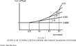
Figures 1 and 2 illustrate the logic of the investment-cash flow test in my context. In these figures, r is the risk-adjusted market interest rate (it is also the rate of return a firm could earn on money if it chooses not to use that money for investment). ICF represents the firm's internal cash flow. If ICF is greater than the firm's desired investment, the firm can self-finance all of its investment and agency problems do not arise. If ICF is less than the desired investment, the firm will seek external financing from banks.
SUPPLY OF FUNDS CURVES UNDER DIFFERENT BANKING SYSTEMS
THE EFFECT OF A CHANGE IN CASH FLOW ON INVESTMENT FOR FIRMS OF DIFFERENT SIZES
The firm will first borrow from the bank from which it faces the lowest external finance premium. This first bank, Bank1, will have the least amount of information asymmetry with the firm among all banks. Limitations in transportation and communication during the period under study imply that Bank1 will be geographically close to the firm. B1 − ICF is the amount of money Bank1 can legally lend to the firm. This amount is limited by the inability of unit banks to attract widespread deposits and regulations prohibiting banks from making loans of more than 10 percent of their capital and surplus to an individual person or corporation. If desired investment is greater than B1, the firm will borrow from another bank. B2 – B1 is the amount of money that the bank with the second most information about the firm can legally lend to the firm, and so on.
Under the assumptions of Modigliani-Miller, the cost of funds is the same regardless of whether it comes from internal or external sources, and the relevant supply curve for the firm is S(MM). More realistically, external financing is not a perfect substitute for internal financing. Banks will charge lenders a premium on the money they borrow, raising the cost of external funding. This premium results from costs of financial distress and information asymmetries between the firm and the lending bank(s). The supply of funds curve becomes upward sloping because rising expected costs of financial distress (as a firm becomes more leveraged) result in an increasing marginal premium charged on funds.
As mentioned previously, when a firm seeks bank financing it will first borrow from a local bank that can gather information about the firm relatively easily. The slope of the supply of funds curve segment associated with the first bank is H, representing the premium for financial distress and asymmetric information. If a firm is not too large, this one bank will be sufficient to meet the firm's financing needs. If branch banking were allowed, the complete supply of funds curve the firm faces would be S(BB). If a firm's demand for funds is greater than the first bank can supply, the firm must seek additional funding from a second bank. The segment of the supply curve between B1 and B2 shows the funding that can be supplied by the second bank. The slope of this segment is steeper (by H′) than the previous segment because information asymmetries are greater between the firm and the second bank than they were between the firm and the first bank. If the firm must borrow from yet a third bank, the slope of the supply curve will increase again (by H″) as the firm and third bank suffer from even larger information asymmetries. The complete supply of funds curve under a unit banking system is given by S(U).
A firm's optimal level of investment (calculated from the firm's expected future profit function) is determined by the intersection of the supply curve with the firm's investment demand curve. Investment demand is likely proportional to firm size so that large firms will have a higher demand for financing than smaller firms. Figure 2 shows three demand curves corresponding to a small firm (D − S), a medium firm (D − M), and a large firm (D − L).
With an internal cash flow of ICFa, the optimal levels of investment chosen by the three firms are I – Sa, I − Ma, and I − La, respectively. If cash flow increases, the supply curve will shift outward by the amount of the increase in cash flow. Suppose that cash flow increases to ICFb in Figure 2. As the curve shifts out, the optimal quantity of investment will increase for each of the firms (to I − Sb, I − Mb, and I − Lb, respectively). It can be seen that investment is sensitive to cash flow and, more importantly, this sensitivity increases with firm size.
The positive relationship between firm size and investment sensitivity to cash flow is a direct result of the unit banking system. Under a nationwide branch banking system, even the largest firms would need to go only to a single bank for financing, no matter how much they wanted to borrow. Accordingly, the supply-of-funds curve facing firms of all sizes under branch banking would be similar to S(BB) from Figure 1. The resulting investment sensitivities to cash flow would generally no longer be increasing in firm size.31
There is some disagreement in the literature as to whether or not having a relationship with a single bank will cause a firm to be less finance constrained than if the firm has relationships with multiple banks or obtained financing from financial markets. As noted previously, Fohlin, “Relationship Banking,” does not find evidence that German firms with a relationship with large German universal banks were less finance constrained than firms without such a relationship. Houston and James, “Do Relationships,” find that firms that have relationships with multiple banks are less finance constrained than firms that have a relationship with only a single bank. They go on to say, however, that their “results suggest that a close banking relationship lowers the cost of external financing for projects in which exclusive reliance on bank financing is feasible” (p. 372). To the extent that the elimination of branch banking restrictions would have increased the ability of individual banks to provide enough funds to entirely finance large projects, their results are consistent with the assumption that large branching banks will lower the cost of funds to large borrowers.
Steven Kaplan and Luigi Zingales present a simple algebraic model of firm investment that further illustrates the relationship between cash flow and firm investment in the presence of information asymmetries.
32 Kaplan and Zingales, “Do Investment-Cash Flow Sensitivities.”
Suppose a firm's return to an investment (
I) is given by the production function
F(
I), where
F′(
I) > 0 and
F″(
I) < 0. Investment can be financed using either internal cash flow (
ICF) or with external funds (
E). The opportunity cost of the internal funds is
r, which can be normalized to one. Because of information asymmetries the cost of external funds includes a premium (
H); the cost function for external funds can thus be written
C(
E, H), where
C(·) is convex in
E. Each firm chooses
I to maximize
The first order condition of equation 1 is
where F1() is the first derivative of F with respect to I and C1 is the partial derivative of C with respect to its first argument. Implicit differentiation of equation 2 gives the effect of internal cash flow on investment
If capital markets are perfect, dI/dICF = 0, because C(·) = 0 and thus C11 = 0. In the presence of asymmetric information, dI/dICF > 0; i.e., investment is sensitive to internal cash flow. Important for the analysis of this article, as C11 increases, holding all else constant, dI/dICF increases. The steeper the supply of funds curve, the larger is C11, and the more sensitive investment is to changes in cash flow. Because branch banking restrictions cause the supply curve to become steeper as loan size increases, investment sensitivity to cash flow should increase with firm size.
33 It is possible that although branching restrictions may have limited the ability of banks to provide large-scale financing, large firms could still have easily raised funds from nonbank sources (such as through the issuance of bonds or equity). If this were the case, then firm investment would not have been constrained by branching restrictions and would therefore not exhibit sensitivity to cash flow. If firm investment is found to be sensitive to cash flow, it provides evidence that these possible alternative sources of funds were unable to overcome financial market imperfections caused, at least in part, by restrictions on branch banking.
The predictions concerning sensitivity of investment to cash flow from Figure 2 and the algebraic model provide a framework with which to test for capital market imperfections resulting from restrictions on branch banking. The basic econometric specification of these tests is given by the following equation
where I is the firm's investment. I is normalized by the firm's beginning of period capital stock to reduce potential problems of heteroskedasticity. x is a set of explanatory variables; αi is a firm specific indicator variable; and γt is a year specific indicator variable. The subscript i denotes the individual firm and t denotes the year. Explicitly, this article uses a fixed effects model of the form used by Fazzari, Hubbard and Petersen
where Q is Tobin's Q and CF is the cash flow of the firm normalized by the firm's beginning of period capital stock. Q is included to control for changes in the investment demand schedule. A cash flow coefficient significantly greater than zero indicates the presence of finance constraints. The more severe the constraints the larger the coefficient.
34 Although there is a large literature that examines investment sensitivity to cash flow as evidence of finance constraints, this methodology is not without controversy. Kaplan and Zingales, “Investment-Cash Flow Sensitivities,” in particular, argue that investment sensitivity to cash flow may result from factors other than firms being finance constrained. For example, managers of large, established firms may have been more conservative and risk-averse than managers of smaller firms and therefore more likely to finance investment using funds obtained from retained earnings than from external sources. It is also possible that investment sensitivity to cash flow may have arisen because managers of larger firms practiced nonoptimizing behavior.
DATA AND SUMMARY STATISTICS
The firm-level data used to estimate the models in this article come from Moody's Analyses of Investments and consist of annual observations for the years 1911–1922. For a firm to be included in the sample it is required that Moody's reported its income statement, balance sheet, and stock prices for at least five consecutive years during the period under study. (In essence, the sample includes every industrial firm for which the data are sufficient to perform the econometric tests).35
Peculiarities and inconsistencies in the data for a small number of firms caused them to be excluded from the data set even if they seemed to meet the requirements for inclusion. For example, it was often the case that firms changed the way they reported information on their income and balance sheets causing the same statistic for a firm in a given year to be listed differently in separate volumes of Moody's. Considerable effort was expended to determine the source of each of these inconsistencies and then correct the problem. Unfortunately for a few firms this was not possible, prohibiting their inclusion in the sample. There are not any identifiable characteristics that caused firms to have these reporting problems; hence their exclusion should not bias the remaining sample. Following a standard practice in the modern finance constraint literature, the 1-percent tails of each variable have also been removed to reduce the possible effects of outliers in the data.
The result is an unbalanced panel of 266 firms with 2,641 observations. The use of an unbalanced dataset serves to lessen potential selection and survivorship biases.
Because Moody's does not directly report the variables used in the regressions it was necessary to determine them from the available data. Cash flow is defined as the sum of net profits plus depreciation normalized by the beginning of period capital stock for the investment analysis or beginning of period total assets for the growth analysis. The capital stock is the sum of property, equipment, machines, and so on. Investment is the firm's net investment determined by the change in capital stock normalized by the beginning of period capital stock. Growth is the percentage change in total assets. Tobin's Q was somewhat harder to measure. The Q-ratio is the market value of a firm divided by the replacement cost of its capital. To calculate a firm's market value, I replaced the book value of the firm's equity outstanding with the market value of the firm's equity (determined by multiplying the number of shares outstanding by the average of the yearly high and low stock price). Then I divided this figure by the book value of the firm's total assets to obtain a measure of average Q for the firm. Stock price change is the percentage change in the average yearly common stock price. All variables are converted to real terms.36
The variables are converted to real terms by deflating them by the Index of the General Price Level as given in NBER series 04051.
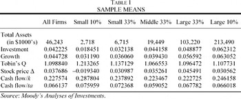
Table 1 presents the sample means of the key variables. The statistics are presented for the entire sample and then for subsets of the observations based upon firm size.37
Firm size was determined using total assets. Individual observations from the same firm were not necessarily placed into the same subset. If a firm experienced growth (or decline) the observations from that firm may have fallen into different categories.
The relationship between net investment and growth is very sensible, and the means for growth are approximately equal to other estimates of manufacturing growth for this period.
38 See NBER series 01007, for example.
Despite the difficulties in measuring Tobin's Q, its sample means also seem to be reasonable. The Q-ratios are slightly greater than unity, fitting well with the positive sample means for net investment and growth.
No distinctive relationship exists for Tobin's Q, changes in stock price, or cash flow across size groups. However, a positive relationship does exist between firm size and both investment and growth. The growth rate for the larger firms was substantially higher than the growth rate of the smaller firms. At first blush, this finding might seem to imply that finance constraints posed less severe problems for large firms than for small firms, but this implication is not justified. It is alternatively possible that large firm growth rates were high because the expected marginal profits from expansion were higher for large firms than for small firms even if large firms faced greater finance constraints than smaller firms. The regression results presented in the next sections provide a clearer insight into whether large firms were facing financing constraints.
INVESTMENT SENSITIVITY REGRESSION RESULTS
Table 2 presents the results of the tests for finance constraints using two separate specifications of equation 4. For each specification the sample was broken into subsets to test for differences in finance constraints based upon firm size.39
Given that there were differences in state branching laws during this period, it would seem obvious to test for differences in firm finance constraints across states. Unfortunately, meaningful tests of this type could not be performed because very few of the firms in the sample were located in states where widespread branching was permitted. A second factor confounding this type of test was that many of the firms in the sample had offices in more than one state, making it difficult to objectively determine the appropriate state classifications. (For example, it was not uncommon for firms to be headquartered in one state, have a financial office in one or more other states, and be incorporated in yet another state).
The estimates of equation 5 are given by the top set of rows of
Table 2; White's heteroskedasticity-consistent standard errors are reported in parentheses. Investment sensitivity to cash flow monotonically increases with firm size, indicating that larger firms faced greater external finance constraints than smaller firms.
40 To confirm that the cash flow coefficients were significantly greater for larger firms than for smaller firms, I pooled the data and estimated a model containing variables for cash flow interacted with dummy variables for firm size. Specifically, I estimated the model Iit = αi + γt + β1Qit + β2CFit × S + β3CFit × M + β4CFit × L + εit, where S, M, and L are indicator variables for firm size (small, medium, and large). An F-test rejected at the 1-percent level the null hypothesis that β2 = β4, indicating that the effect of cash flow on firm investment was significantly greater for larger firms than for smaller firms. Similar results were found when pooled regressions were estimated for the additional investment and growth models presented later in this article.
Three things should be noted concerning these results and the firms used in the sample. First, these results are quite different from what one would expect to find in a study of modern firms. Researchers using recent data would most likely expect smaller firms to be more constrained than larger firms. This is because larger firms are typically better-known than smaller firms; therefore larger firms generally suffer less from information asymmetries than do smaller firms. This is likely also the case for firms in this study, which makes the finding that large firms have larger cash flow coefficients than smaller firms even more striking. The hindrances imposed by branch banking restrictions were potentially so severe as to overwhelm the benefits of information dissemination firms obtained from being large. The second thing to note is that all of the firms in this study were relatively large compared with all other firms existing at the time.41
It is to be expected, however unfortunate, that the sample of firms listed in Moody's is comprised mostly of the largest firms existing at the time. Similar limitations still exist in modern firm-level data.
If data were available for much smaller firms, it would likely be found that they suffered from finance constraints similar to those experience by their small counterparts today. Finally, readers familiar with the finance constraint literature studying modern firms may find the cash-flow coefficients lower than expected. This is likely the result of using net investment rather than gross investment as the dependent variable.
For the first specification of the regression model, Tobin's Q is not a significant determinant of investment.42
A possible explanation for the poor performance of Tobin's Q is that fluctuations in the price of capital goods over the period caused it to be measured incorrectly. Due to limitations of the data it was not possible to construct a series of the real capital stock for each firm that could then have been used to derive a potentially more correct measure of Tobin's Q.
To better control for changes in investment not resulting from changes in the supply of funds, a second specification of the model uses changes in common stock prices instead of Q to capture shifts in the investment demand curve. The stock price changes seem to be a better determinant of investment than Q, and the correlation between firm size and the cash flow coefficients remains positive, so the results again indicate that large firms faced greater external finance constraints than smaller firms.
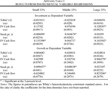
43 It is possible that shocks to investment are not independent of shocks to contemporaneous cash flow, resulting in spurious correlations between the two. This might occur if investment in one period is able to affect cash flow in the same period. For example, if an investment project is undertaken in January it may cause increased cash flow in December. Specifications of the model that used lagged cash flow as an instrument for current cash flow to remove the possibility of such feedback were also estimated. The results of these specifications (presented in the Appendix) show that, although no longer monotonically increasing with firm size, investment sensitivity to cash flow was still higher for larger firms compared to smaller firms.
TESTING FOR FINANCE CONSTRAINED GROWTH
The investment-cash flow sensitivity results presented provide interesting evidence that large firms' investment in capital was more finance constrained than the investment of smaller firms. This section presents a separate test that firm growth was finance constrained. Growth is measured by the percentage change in total assets and is likely to be more accurately measured than investment for these data.44
Investment is determined solely from the capital stock whereas growth is determined by the capital stock plus all other firm assets. These assets include items such as cash and inventories which are easier for firms to report accurately.
The basis of this test, developed by Robert Carpenter and Bruce Petersen, is illustrated by
Figure 3.
45 Carpenter and Petersen, “Is the Growth.”
Although there are a few key differences, it is similar to the model presented in
Figure 2. Cash flow is again measured along the horizontal axis and the supply of funds curve is the same as in
Figure 2. The downward sloping curve now represents the firm's marginal revenue of expansion schedule (
MRex) rather than investment demand. This measures the marginal return of expanding all of the firm's assets, not just fixed investment. Change in total assets (in other words, growth) is also measured on the horizontal axis.
THE EFFECT OF A CHANGE IN CASH FLOW ON GROWTH FOR FIRMS OF DIFFERENT SIZES
The MRex curve measures the marginal returns to expanding a firm's assets, where the composition of all assets (and other inputs) has been optimally selected. Firms will expand until the MRex equals the marginal cost of expanding. This occurs where the MRex curve intersects the supply of funds curve. Analogous to the investment model presented previously, if a firm faces an upward sloping supply of funds curve, an increase in cash flow will cause an increase in its expansion. Or put another way, costs of external finance cause the growth of the firm's total assets to depend upon internal cash flow. The sensitivity of growth to cash flow again depends upon the slope of the supply-of-funds curve.
Because the supply-of-funds curve is the same as in the investment analysis, larger firms will again face steeper supply curves than smaller firms. The implication is that larger firms' growth will be more dependent upon internal cash flow than the growth of smaller firms. This is illustrated in Figure 3 by the change in internal cash flow's effect on the optimal level of growth for three firms of different sizes. MRex − S, MRex − M, and MRex − L are the marginal revenue of expansion curves for a small, medium, and large firm, respectively. As internal cash flow increases from ICFa to ICFb, firm growth increases from G − ia to G − ib for each firm. The change in firm growth with respect to a change in cash flow increases with firm size. Carpenter and Petersen note that growth sensitivity to cash flow is also a function of the slope of the marginal revenue of expansion curve. Under perfect competition, a firm's MRex curve is flat, whereas firms with market power have steeper MRex schedules. Holding all else constant, growth sensitivity to cash flow should be greater for firms in competitive markets than for firms with market power. Carpenter and Petersen also demonstrate that the presence of finance constraints for a perfectly competitive firm will result in a growth sensitivity to cash flow coefficient of unity.
To test the prediction that growth sensitivity to cash flow increases with firm size, fixed effects models of the basic form:
are estimated. Growth is the change in firm's total assets normalized by beginning of period total assets; the other variables are as defined for equation 5.
GROWTH SENSITIVITY REGRESSION RESULTS
Table 3 presents the results from the tests of finance-constrained growth. Corresponding to the investment tests, two sets of model specifications are estimated. The results from estimating equation 6 are given in the first set of rows in Table 3. The cash flow coefficients for the smaller firms are significantly less than the coefficients of larger firms. This result indicates that larger firms' growth was more finance constrained than smaller firms' growth. This finding is especially striking under the assumption that larger firms have more market power than smaller firms, which would bias the coefficients for larger firms downward. The results of the first set of regressions is somewhat tainted by the presence of significantly negative coefficients for Tobin's Q. To better control for changes in the marginal revenue of expansion schedule, the model is reestimated using percentage change in common stock price in place of Tobin's Q. The direct relationship between firm size and growth sensitivity is again evident in the estimates.46
As with the investment models, additional sets of regressions were estimated that used lagged cash flow as an instrumental variable to eliminate possible reverse causation between growth and cash flow. The results of these regressions, presented in the Appendix, also indicate that growth sensitivity to cash flow increased with firm size.
CONCLUSION
The results of this article present evidence that restrictions on branch banking hindered the development of large-scale American enterprises in the early twentieth century. Lacking the capability to branch and faced with regulations affecting the maximum size of loans, banks were unable to provide loans to cover the massive amount of financing required by large firms. As a result, the firms were forced to obtain external funding from alternative sources such as bonds, commercial paper, or equity. This article in a sense examines how effectively these other sources provided financing. If these other sources of funding were imperfect and costly, large firms would have preferred to self-finance their investment and growth more so than relatively smaller firms. Tests using firm-level panel data support this hypothesis. Regression results demonstrate that investment and growth sensitivity to changes in cash flow increased with firm size, suggesting an inability of the financial system to provide adequate external financing to very large firms.47
These findings echo Calomiris, who writes, “The claim is not that America failed to grow and prosper, but that large-scale industrial investment was stunted relative to its potential by a faulty financial system.” “Costs,” p. 256.
The evidence that branching restrictions may have caused large firms to face finance constraints may help to explain several changes that began to occur in the American banking system during the 1920s. One such change already mentioned was a merger movement in the banking industry. A second change that may have been fostered by the banking system's attempts to overcome the lending limitations caused by branching restrictions was the rise of banks' securities affiliates.48
Although there were several ways to organize a securities affiliate, they were all basically incorporated under general laws of incorporation instead of under banking and trust laws, giving them the freedom to engage in many activities prohibited to the commercial banks themselves. (White, “Before Glass-Steagall,” p. 35).
These affiliates allowed banks to provide financing to firms by underwriting stock and bond issues. Securities affiliates proved effective at distributing securities, and the number of banks operating securities affiliates grew rapidly from 18 in 1922 to 180 in 1930.
49 Peach, “Securities Affiliates,” p. 83.
A key benefit of securities affiliates is that they were able to gather funds from much larger geographic areas than commercial banks. As White relates, securities affiliates “allowed banks to circumvent geographical restrictions on their activities. Unlike national banks, an investment company could establish branches without limit; and some affiliates had offices across the country.”
50 White, “Before Glass-Steagall,” p. 37. White also provides a brief sample showing the number of branches operated by several notable securities affiliates: “In 1930, National City Company had 60 branches; Chase Securities Corporation, 26; First National Old Colony Corporation, 17; and Continental Illinois Company, 12” (p. 37). It should be added, though, that there were securities affiliates that did not operate any branches. Peach, “Securities Affiliates,” (p. 104).
An interesting possible extension of the research of this present article would be to study the effects of these securities affiliates to see if they reduced firm finance constraints during the 1920s.
51 The finding by Ramirez, “Did Glass-Steagall,” that the Glass-Steagall Act's separation of commercial from investment banking increased investment sensitivity to cash flow for firms with bank affiliations supports the idea that securities affiliates were able to reduce firm finance constraints.
This article is a revised version of a chapter from my unpublished Ph.D. dissertation. I am deeply grateful to Steven Fazzari, Sukkoo Kim, Douglass North, and John Nye for their guidance and supervision as I conducted this research. I also wish to thank seminar participants at Washington University in St. Louis and Grand Valley State University as well as two anonymous referees for their helpful comments and suggestions. Any remaining errors are solely attributable to the author.