a. Modeling a two-part wine marketFootnote ²

Those differences in demand elasticities suggest that the demand curve for fine wine would move out faster than that for non-premium wine in the course of growth in global income and population. That difference would be greater the more existing wine consumers “premiumize” by transitioning away from non-premium and toward fine wine, and the more young people begin their consumption of wine at higher price points than did previous generations.

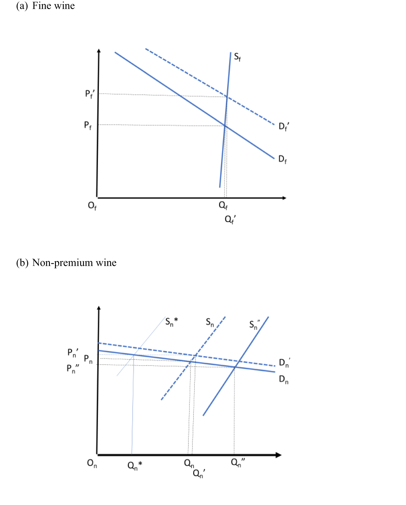
That situation is depicted in Figure 1, assuming the demand for both wine types expands (as happened in the first three decades following World War II, for example). Assuming no shifts in the supply curves and the demand curves shift out from D_f and D_n to D_f′ and D_n′, the price and quantity of both wines would rise as incomes and the population rise globally, but the proportional price (quantity) rise for fine wine would be greater (smaller) than that for non-premium wine.

Figure 1.

The changing global markets for non-premium and fine wines. (a) Fine wine, (b) non-premium wine.

Figure 1 Long description

The market for fine wine. The vertical axis represents price and the horizontal axis represents quantity. Initially, the equilibrium is at P subscript f and Q subscript f, where the demand curve D subscript f intersects the supply curve S subscript f. After the demand curve shifts to D subscript f prime, the new equilibrium is at P subscript f prime and Q subscript f prime, indicating an increase in price and quantity. Panel B shows the market for non-premium wine. The vertical axis represents price and the horizontal axis represents quantity. Initially, the equilibrium is at P subscript n and Q subscript n, where the demand curve D subscript n intersects the supply curve S subscript n. After the demand curve shifts to D subscript n prime, the new equilibrium is at P subscript n prime and Q subscript n prime, indicating a smaller increase in price and a larger increase in quantity compared to fine wine. The graphs illustrate that the proportional price rise for fine wine is greater than that for non-premium wine, while the quantity increase is smaller for fine wine.

If, however, preferences were to alter such that the demand for non-premium wine shrank (as happened in the final two decades of last century), then its price and quantity would fall. In Figure 1(b), think of a shift from D_n′ to D_n. In that case, the supply curve for non-premium wine would need to shift to S* for the price of that wine to return to what it was before its demand shrank. Its output would then be Q_n*.

If the global supply curve for non-premium wine were instead to shift out (as happened with the rapid expansion of branded commodity wine production in several New World countries from the 1990s), that would add to the fall in the relative price of non-premium wine. Production of non-premium wine would increase to Q_n” and its price would drop to P_n”, reducing the profitability of traditional producers of non-premium wine.

Figure 1 could also represent the markets for an individual country, by assuming the demand curves are for the sum of domestically produced and exported local wines. Even for a small country, those demand curves would not be horizontal insofar as that country's wines are differentiated to some extent from those of other countries. The supply curves for that country would include that available for importing and so would be much more elastic than those shown in Figure 1 for the world as a whole. But again, that individual country's supply curve for the world's finest/rarest wines would be more inelastic than that for non-premium wine. Indeed, the latter would be close to horizontal because of the closer substitutability between this and other countries’ non-premium wines (and also beers, spirits, and other stimulants).

Differing changes across countries and over time in the costs of producing, marketing, and transporting non-premium and fine wines, and in both most-favored-nation and preferential tariffs on other countries’ imports of exporting-countries’ wines, can alter the international competitiveness of each country's vignerons in their domestic and export markets. An important shifter for wine producers, particularly in non-U.S. countries outside the Euro zone, is their country's real exchange rate: if it were to appreciate (for example, because of a mining export boom), that would lower the competitiveness of that country's vignerons because (a) the local-currency prices of their exported wines, and of foreign wines imported into their country, would fall and (b) some mobile resources such as labor would be attracted to the expanding mining sector or to the sector producing nontradable products (Corden, Reference Corden1984) —and conversely for a real depreciation.

b. Broadening to all alcoholic beverages

For historical reasons, individual countries—even ones with the same per capita income—have differed in their mixes of wine, beer, and spirits consumption and production. One contributor to the latter has been differences in climate. Wine grapes grow well only in temperate regions between the 30° and 50° latitudes; and, in the coolest climates, spirits typically were preferred to and cheaper to produce with local crop products than beer. As a result, in the early 1960s the world's countries could be clearly separated according to whether their alcohol consumption was wine-, beer-, or spirits-focused (Holmes and Anderson, Reference Holmes and Anderson2017).Footnote ³ Since then, however, with the drop in the costs of internationally transporting goods, fashions and information, one should expect similar-income countries to have become more similar in their mix of alcohols consumed, according to Stigler and Becker (Reference Stigler and Becker1977).

a. The 1970s’ pivot in global wine consumption

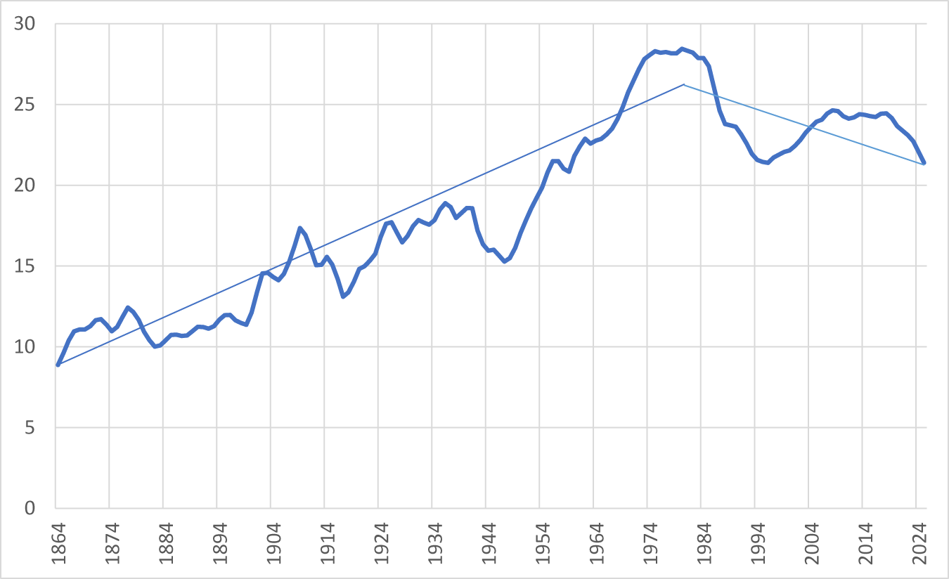
For more than a century up to the 1970s, the volume of global wine consumption cycled around a rising long-run trend, dropping well below trend just in the economic depression of the 1890s and during World Wars I and II. Since then, however, it has arguably cycled around a downward trend (Figure 2). It fell steeply from the early 1980s to the mid-1990s thanks to numerous national campaigns aimed at curbing alcohol consumption. The upturn during the next 15 years was due to the income growth associated with an acceleration of globalization plus the broadcasting in 1991 on the CBS national U.S. television program 60 Minutes of a story that has become known as the French Paradox.Footnote ⁴ But that then flatlined when the global financial (GFC) crisis hit in 2008. It would have gone into decline had the China market not grown over the next dozen years. Its growth spurt was short-lived, though: China's market began shrinking from the late 2010s and is now expected to grow only slowly from a much-reduced base (Anderson Reference Anderson2025b).

Figure 2.

Global beverage wine consumption, 1862–2025 (billion liters, 3-year average to year shown).

Source: Anderson and Pinilla (2026).

Certainly, there have been some recent short-term shocks. The first half of the 2020s decade saw COVID-19 and some geopolitical surprises, but hopefully they will prove to be no more than medium-term dampeners. Earlier than that, the GFC of the late 2000s lowered consumer confidence and led to globalization plateauing through the 2010s. That, too, temporarily lowered the growth in global demand for many goods, including wine.

However, much more worrying for the wine industry is the long-run trend in global alcohol consumption and wine's share of that, plus changes in consumption within the wine category.

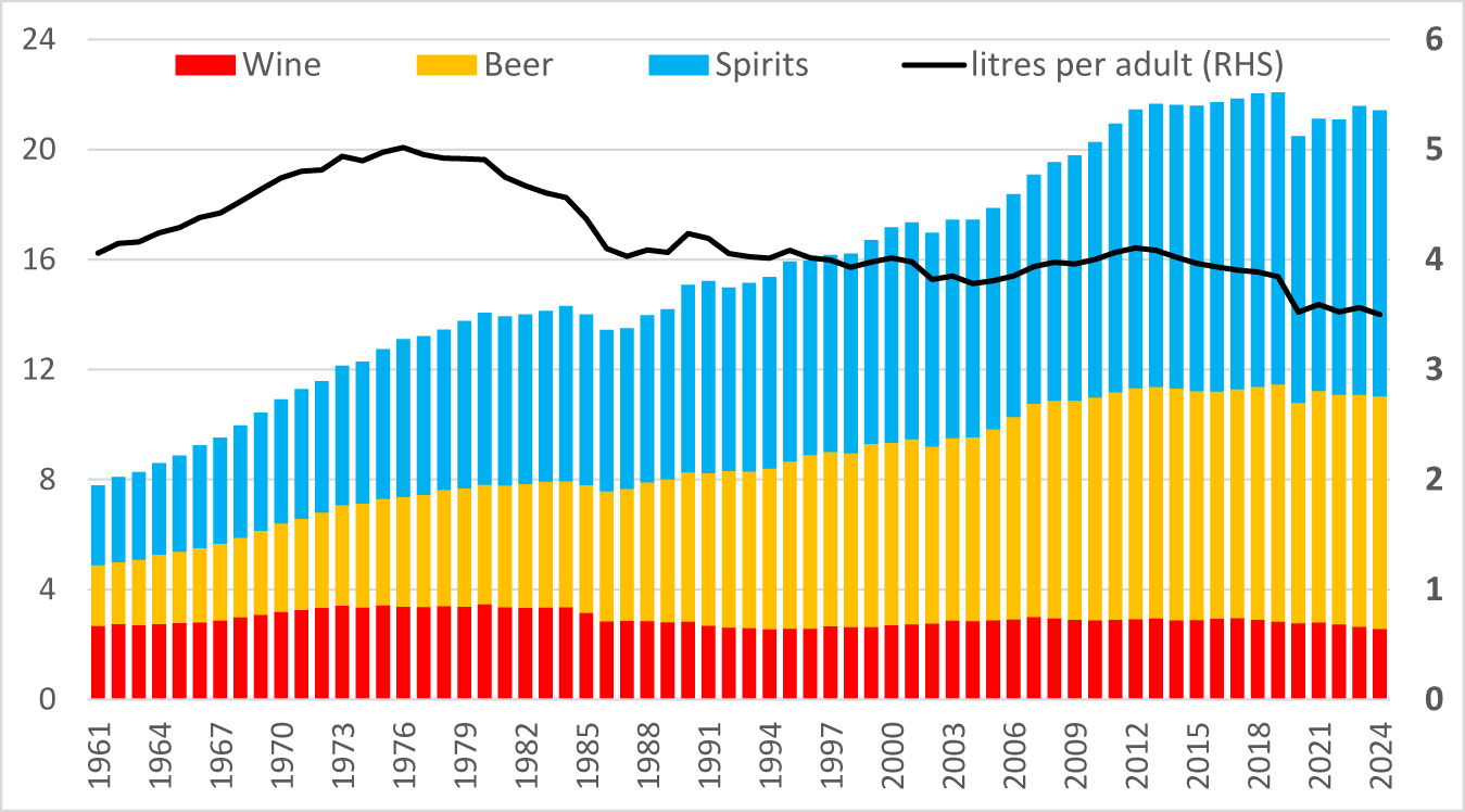
The world's total consumption of alcohol has plateaued since the GFC, and alcohol consumption per adult peaked five decades ago and has fallen 30% since then. Yet the volumes of global beer and spirits consumption have each doubled since the early 1960s while wine consumption has fallen by one-quarter (Figure 4). That has brought wine's share of global alcohol consumption down from above one-third in the early 1960s to below one-eighth since 2023.

Figure 3.

Global consumption of alcohol, total and per adult, 1961–2025 (billion liters and liters).

Figure 3 Long description

Legend text: Wine, Beer, Spirits, litres per adult left parenthesis RHS right parenthesis. Horizontal axis: years, with labeled ticks 1961, 1964, 1967, 1970, 1973, 1976, 1979, 1982, 1985, 1988, 1991, 1994, 1997, 2000, 2003, 2006, 2009, 2012, 2015, 2018, 2021, 2024. Left vertical axis: numeric scale from 0 to 24. Right vertical axis: numeric scale from 0 to 6. Stacked bars: one stacked bar per year from 1961 to 2024. Each bar is segmented into Wine at the bottom, Beer in the middle and Spirits at the top. The total stacked height increases from the early years to the later years, with the tallest totals occurring in the mid to late 2010s and early 2020s, then a small drop and partial recovery by 2024. Category patterns in the stacked bars: Wine forms a smaller bottom segment that rises in the earlier decades and then becomes flatter and slightly lower in later decades. Beer forms a middle segment that grows across the timeline and becomes one of the largest segments in the later years. Spirits forms the top segment and increases notably from the earlier years to the later years, contributing to the higher totals in the 2010s and early 2020s. Line series: a single line labeled litres per adult left parenthesis RHS right parenthesis, read against the right vertical axis scale 0 to 6. The line rises from the 1960s into the 1970s, then trends downward through the 1980s and 1990s, shows smaller rises and falls around the 2000s and 2010s and declines again into the early 2020s, ending lower by 2024 than its earlier peak.

Source: Anderson and Pinilla (2026).

Figure 4.

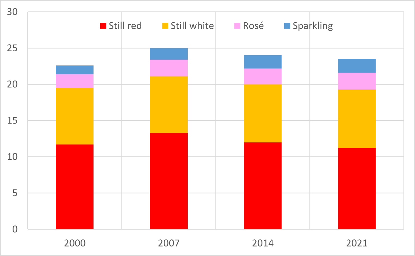
Volumes of still red, still white, rosé, and sparkling wines in global wine consumption, 2000–2021^a (billion liters).

aThe start and end years for volumes of sparkling wine are 2002 and 2018.Source: OIV (2020, 2023).

b. The move away from reds and to lower-alcohol wines this century

Within the wine category, the share of still reds in global wine consumption has fallen over the past two decades as the shares of lower-alcohol wines have risen, notably still whites, rosé, and sparkling wines (Figure 4).

While this decline in red demand began two decades ago, it has yet to be reflected in a fall in the global area of red wine grapes. According to Anderson, Nelgen, Puga, et al. (Reference Anderson, Nelgen and Puga2026), the red-bearing area rose from 2.22 million hectares in 2000 to 2.34 million in 2016 and 2.35 million in 2023 (which was also the year in which California's bearing area of red varieties peaked). This is but an example of the slow response of vine plantings to changes in wine market demand.

c. The move away from non-premium wines and the accumulation of surpluses

Over the period 2013–2022, according to International Wine and Spirits Research (IWSR), the value of global premium wine sales grew at 3.1% (and volume at 1.7%) per year, while the value of global non-premium wine sales shrank at 2.2% per year (where IWSR's division between the two categories is a retail price of US$10 per 75cl bottle or equivalent).Footnote ⁵

An unfortunate feature of the mid-2020s, and a key symptom of the current crisis, is a huge surplus of non-premium red wine in numerous countries in both the northern and southern hemispheres. In Australia, for example, the surplus over and above normal stocks has amounted to more than a year's production, some of it three or more years old; and attempts in 2026 to dispose of it as bulk wine exports have returned less than 60 U.S. cents a liter to stockholders. In California, some bulk Pinot Noir has even been given away by a winery needing an extra empty tank for the 2026 harvest.

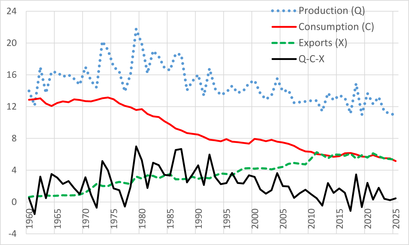
The global decline in demand for non-premium wine began much earlier than the present decade. In fact, most of the decline in the wine consumed within France, Italy, and Spain since the mid-1970s (see Figure 5) has been non-premium. Production there declined only slowly and with a long delay, so surpluses began accumulating in the European Union (EU). The surpluses were reduced periodically with the help of EU subsidies for their distillation into industrial alcohol, plus wine export subsidies. But those subsidies created a moral hazard: winegrowers were inclined to reduce wine production less than if there had been no such subsidization.Footnote ⁶ The extent of this excess production over and above those three countries’ beverage consumption in the past half century is non-trivial (Figure 5). But past subsidies are not the only contributor to the current surplus and to the crisis more broadly. We turn now to consider other contributors.

Figure 5.

Volumes of wine produced, consumed and exported by France, Italy, and Spain, 1960–2025 (billion liters)^a.

Figure 5 Long description

Legend: Production (Q) shown with dotted markers. Consumption (C) shown as a solid line. Exports (X) shown as a dashed line. Q minus C minus X shown as a solid line. Horizontal axis: years, labeled 1960 to 2025. Horizontal axis range: 1960 to 2025. Vertical axis: unlabeled. Vertical axis range: negative 4 to 24. Production (Q) values read from the plotted markers at labeled years: (1960, 13), (1965, 16), (1970, 15), (1975, 18), (1980, 21), (1985, 17), (1990, 15), (1995, 14), (2000, 15), (2005, 14), (2010, 13), (2015, 13), (2020, 12), (2025, 11). Consumption (C) values read from the line at labeled years: (1960, 13), (1965, 12), (1970, 13), (1975, 13), (1980, 12), (1985, 10), (1990, 8), (1995, 8), (2000, 8), (2005, 7), (2010, 6), (2015, 6), (2020, 6), (2025, 5). Exports (X) values read from the dashed line at labeled years: (1960, 1), (1965, 1), (1970, 1), (1975, 2), (1980, 3), (1985, 3), (1990, 3), (1995, 4), (2000, 4), (2005, 4), (2010, 5), (2015, 6), (2020, 6), (2025, 5). Q minus C minus X values read from the line at labeled years: (1960, 0), (1965, 3), (1970, 2), (1975, 2), (1980, 6), (1985, 4), (1990, 4), (1995, 3), (2000, 3), (2005, 2), (2010, 1), (2015, 1), (2020, 0), (2025, 0). Production (Q) shows higher values than consumption (C) across the full year range, with a high point around 1980 at 21 and lower values near 2025 at 11. Consumption (C) declines from about 13 in 1960 to about 5 in 2025. Exports (X) rise from about 1 in 1960 to about 6 around 2015 to 2020, then about 5 in 2025. Q minus C minus X fluctuates around 0 to 6, with a higher point around 1980 at 6 and values near 0 around 2020 to 2025.

aThe black solid line represents the volume of local wine produced each year, net of the volume sold at home or abroad.Source: Anderson and Pinilla (2026).

d. Wine's globalization and new world export take-offs

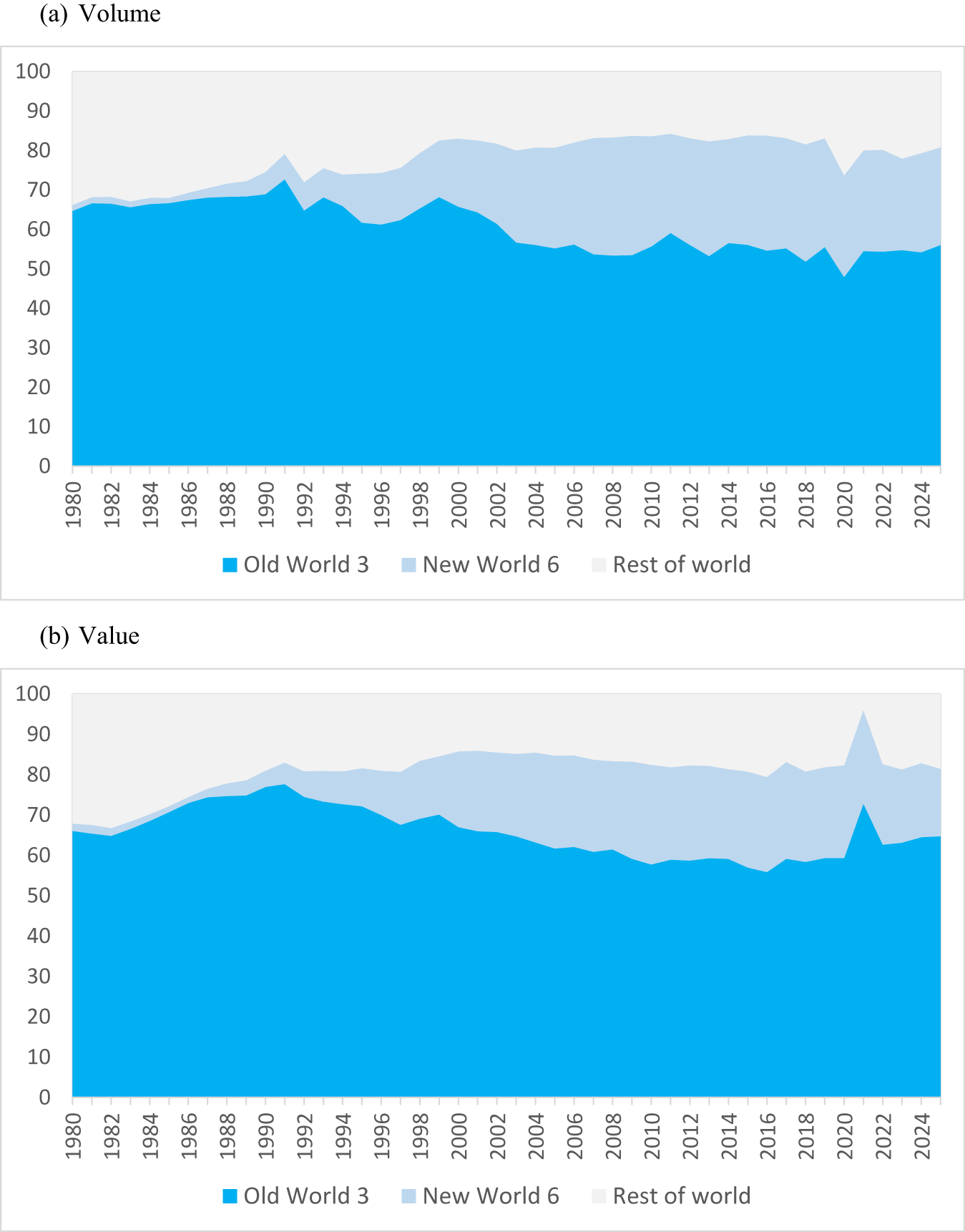
From 1970, when less than 10% of the world's wine production was exported, three forces gradually contributed to a rise in that export share. One was in response to wine consumption peaking in the key producing countries of France, Italy, and Spain. During the 1950s and 1960s, they together accounted for almost 60% of global wine consumption. But after their per capita consumption peaked in the mid-1970s, it fell steadily thereafter—and much faster than did their wine production. Exporting became one of the ways to reduce the accumulating surpluses. But despite EU export and distillation subsidies, those exports were unable to grow rapidly enough to avoid the bloc's surplus accumulating (Figure 6).

Figure 6.

Shares of world wine export volume and value, Old World, New World and Rest of World^a 1980–2025 (%). (a) Volume, (b) value.

Figure 6 Long description

The stacked area graph A has the horizontal axis labeled 1980 to 2024. The vertical axis shows 0 to 100. Legend labels: Old World 3, New World 6, Rest of world. The stacked areas start near 1980 at about 65 for Old World 3, about 2 for New World 6 and about 1 for Rest of world. Around 1990 the Old World 3 area is about 70, with New World 6 about 2 and Rest of world about 1. Around 2000 the Old World 3 area is about 65, New World 6 about 15 and Rest of world about 2. Around 2010 the Old World 3 area is about 55, New World 6 about 25 and Rest of world about 3. Around 2020 the Old World 3 area is about 50, New World 6 about 30 and Rest of world about 5. At 2024 the Old World 3 area is about 55, New World 6 about 25 and Rest of world about 2. The stacked area graph B has the horizontal axis labeled 1980 to 2024. The vertical axis shows 0 to 100. Legend labels: Old World 3, New World 6, Rest of world. The stacked areas start near 1980 at about 65 for Old World 3, about 2 for New World 6 and about 1 for Rest of world. Around 1990 the Old World 3 area is about 78, New World 6 about 3 and Rest of world about 1. Around 2000 the Old World 3 area is about 67, New World 6 about 18 and Rest of world about 2. Around 2010 the Old World 3 area is about 60, New World 6 about 23 and Rest of world about 2. Around 2020 the Old World 3 area is about 58, New World 6 about 25 and Rest of world about 2. Around 2021 the Old World 3 area rises to about 72, with New World 6 about 10 and Rest of world about 2. At 2024 the Old World 3 area is about 65, New World 6 about 17 and Rest of world about 2.

a“Old World 3” is France, Italy, and Spain; “New World 6” is Argentina, Australia, Chile, New Zealand, South Africa, and the United States.Source: Anderson and Pinilla (2026).

A second force contributing to the rise in the share of wine's production that is exported was the gradual fall in ocean transport costs and governmental trade-related policies restricting wine imports. Those developments contributed to globalization generally.

A third force was the emergence and then rapid expansion of wine production in and wine exports from several New World countries from the 1990s. Argentina, Australia, Chile, New Zealand, South Africa, and the United States together accounted for just 1% of the volume and value of global wine exports in 1985. But by the time of the GFC in the late 2000s, their shares peaked at 25% by value and 30% by volume. By then, the combined shares of France, Italy, and Spain had fallen to 58% by value and 53% by volume (Figure 6). The volume of global wine exports had more than doubled over those four decades, but even so these changed shares represent an erosion of Old World competitiveness.

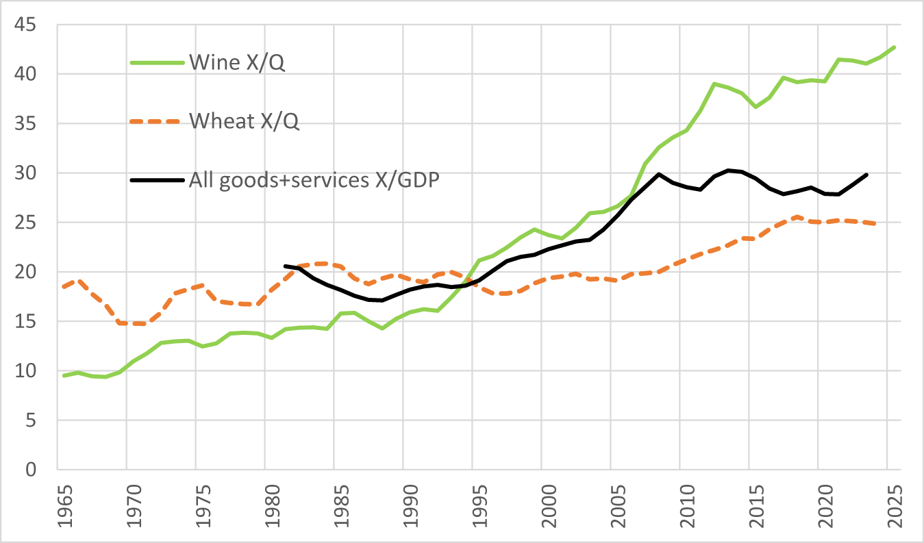
These three forces contributed to a rapid rise in the share of global wine production that is exported. For wine in aggregate, that share rose from 10% to 43% between 1965 and 2025. By contrast, over that same period the share for wheat rose from 19% to just 25%, and for all products from less than 20% to just 30% (Figure 7).

Figure 7.

Exports as a % of production (X/Q) for wine, wheat, and all products, 1965–2025 (3-year average to year shown).

Source: Anderson and Pinilla (2026), World Bank (2026a) and, for wheat, FAOSTAT.

Even though each country's wines are differentiated to some extent from those of other countries, they all now compete in the more or less open markets of all countries. Of course, excise and import taxes differ across countries, but if they do not change, then the domestic prices of fine and non-premium wines can be expected to move in the same directions as in the global market. Wine grapes are too perishable to be traded internationally, of course, but their prices now tend to closely follow the prices of the wines into which they are destined. This has become increasingly so as the flow of wine across national borders has increased with globalization, ensuring that the current crisis is adversely affecting vignerons in virtually all trading countries, and especially those producing less-differentiated non-premium (particularly high-alcohol red) winegrapes and wine. The latter are treated by some consumers as little more than the cheapest form of alcohol available to them, in which case their demand is heavily dependent on the local retail prices of the cheapest beers and spirits.

e. Winegrape price trends

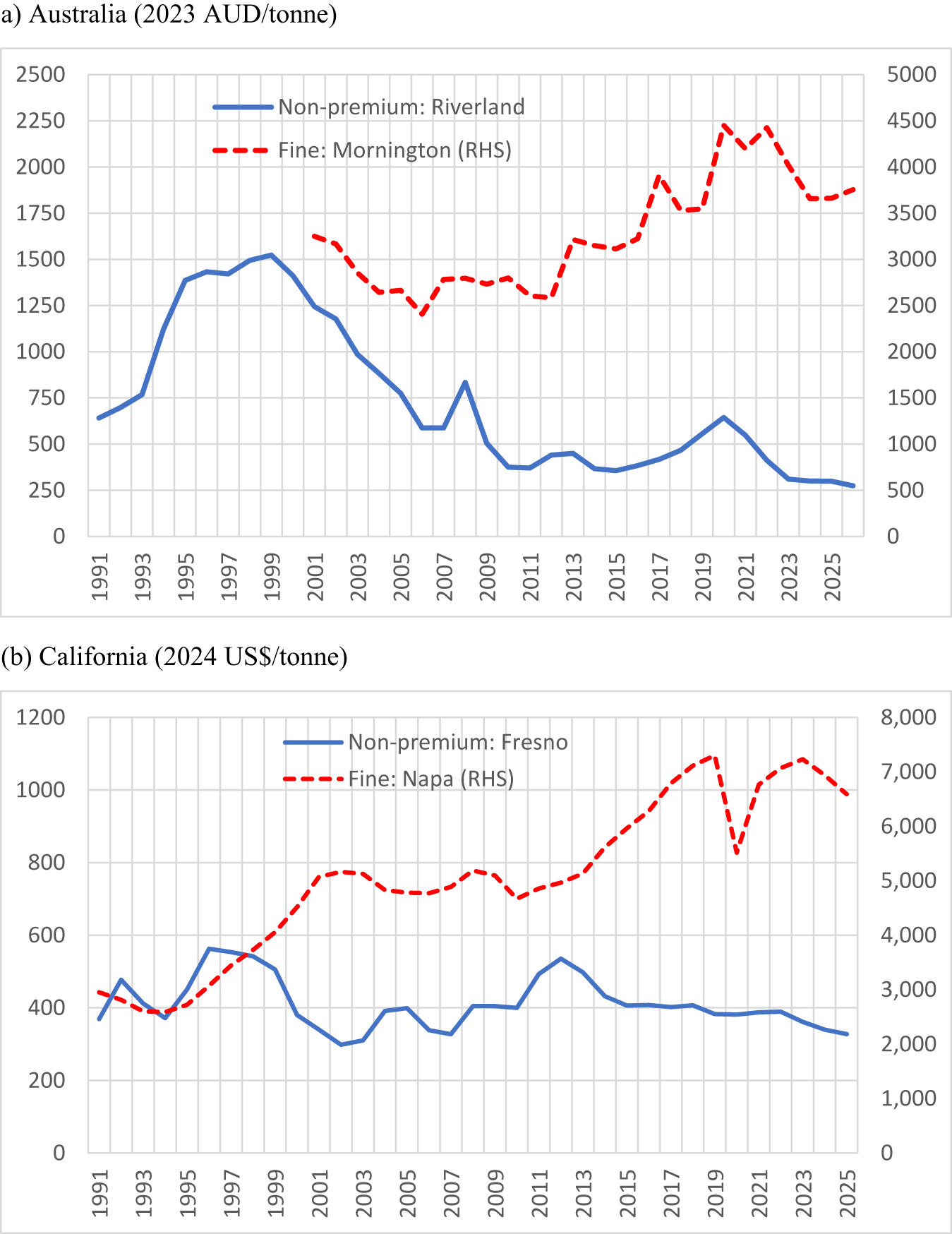
As suggested in Section II, the shifts in demand and supply for non-premium versus fine wine described in this section should show up as price declines for non-premium wine both in real terms and relative to the price of fine wine. That in turn should be reflected in the prices of winegrapes. While it is difficult to capture broad indicators of such price changes, one set of specific prices is presented here by way of illustration: average prices of winegrapes from well-known wine regions in Australia and California. They are shown in Figure 8 for one hot inland irrigated non-premium region and one cooler fine-wine region for each of Australia and California. In each case, the two prices have diverged considerably this century. In Australia's hot Riverland, prices rose rapidly in the 1990s, stimulating the export-focused output growth mentioned above, before they fell substantially in the 2000s. In California's hot Fresno region, the price decline since the latter 1990s has been more gradual, but downwards nonetheless in real terms.

Figure 8.

Real price of representative non-premium and fine wine grapes, Australia and California, 1991– 2026. (a) Australia (2023 AUD/tonne), (b) California (2024 US$/tonne).

Figure 8 Long description

A multi line graph titled, a) Australia (2023 AUD slash tonne). Legend labels, Non premium: Riverland and Fine: Mornington (RHS). Riverland is drawn as a solid line. Mornington is drawn as a dashed line. The horizontal axis shows years from 1991 to 2025. The left vertical axis ranges from 0 to 2500 and represents price in 2023 Australian dollars per tonne. The right vertical axis ranges from 0 to 5000 and represents price in 2023 Australian dollars per tonne. Non premium: Riverland coordinate pairs: (1991, 650), (1992, 700), (1993, 750), (1994, 1100), (1995, 1400), (1996, 1450), (1997, 1450), (1998, 1500), (1999, 1500), (2000, 1350), (2001, 1200), (2002, 1000), (2003, 900), (2004, 750), (2005, 600), (2006, 600), (2007, 800), (2008, 500), (2009, 400), (2010, 400), (2011, 450), (2012, 450), (2013, 400), (2014, 400), (2015, 420), (2016, 450), (2017, 500), (2018, 550), (2019, 650), (2020, 550), (2021, 400), (2022, 300), (2023, 300), (2024, 300), (2025, 280). Fine: Mornington (RHS) coordinate pairs: (2001, 3200), (2002, 3000), (2003, 2700), (2004, 2700), (2005, 2400), (2006, 2800), (2007, 2800), (2008, 2800), (2009, 2700), (2010, 2700), (2011, 2600), (2012, 3200), (2013, 3100), (2014, 3100), (2015, 3200), (2016, 3800), (2017, 3500), (2018, 3500), (2019, 4500), (2020, 4200), (2021, 4500), (2022, 4000), (2023, 3600), (2024, 3600), (2025, 3800). Key values from the plotted points: Riverland reaches 1500 in 1998 and 1999, then declines to 280 by 2025. Mornington reaches 4500 in 2019 and 2021 and is 3800 in 2025. The image B showing a multi line graph titled, (b) California (2024 US dollar slash tonne). Legend labels, Non premium: Fresno and Fine: Napa (RHS). Fresno is drawn as a solid line. Napa is drawn as a dashed line. The horizontal axis shows years from 1991 to 2025. The left vertical axis ranges from 0 to 1200 and represents price in 2024 dollars per tonne. The right vertical axis ranges from 0 to 8000 and represents price in 2024 dollars per tonne. Non premium: Fresno coordinate pairs: (1991, 380), (1992, 470), (1993, 400), (1994, 380), (1995, 450), (1996, 560), (1997, 550), (1998, 520), (1999, 380), (2000, 320), (2001, 300), (2002, 320), (2003, 400), (2004, 400), (2005, 350), (2006, 330), (2007, 400), (2008, 400), (2009, 400), (2010, 500), (2011, 530), (2012, 500), (2013, 430), (2014, 410), (2015, 410), (2016, 400), (2017, 400), (2018, 390), (2019, 390), (2020, 390), (2021, 390), (2022, 380), (2023, 360), (2024, 340), (2025, 330). Fine: Napa (RHS) coordinate pairs: (1991, 3000), (1992, 2800), (1993, 2700), (1994, 2800), (1995, 3000), (1996, 3300), (1997, 3600), (1998, 4000), (1999, 4500), (2000, 5000), (2001, 5200), (2002, 5200), (2003, 5000), (2004, 4800), (2005, 4800), (2006, 4900), (2007, 5200), (2008, 5200), (2009, 4800), (2010, 5000), (2011, 5100), (2012, 5200), (2013, 5600), (2014, 6000), (2015, 6200), (2016, 6600), (2017, 7000), (2018, 7200), (2019, 5000), (2020, 6500), (2021, 7000), (2022, 7200), (2023, 7000), (2024, 6800), (2025, 6500). Key values from the plotted points: Fresno reaches 560 in 1996 and 530 in 2011 and is 330 in 2025. Napa reaches 7200 in 2018 and 2022, drops to 5000 in 2019 and is 6500 in 2025.

Source: Anderson and Puga (2023, 2024).

a. Why the decline in alcohol consumption, especially wine (particularly non-premium)

The decline in global alcohol consumption per adult since the 1970s had been more than offset by population growth until the early 2010s but, for more than a dozen years now, total alcohol consumption has plateaued (Figure 3). Numerous reasons have been suggested including a greater focus on health and well-being spurred on by anti-alcohol lobbying, a decline in consumer confidence and slower income growth due to a retreat from globalization since the GFC of the late 2000s, the arrival of new alternative stimulants such as GLP-1 and other weight-loss drugs and legalized marijuana in some jurisdictions (consumers typically prefer a wider variety of goods as their incomes rise), and a decline in face-to-face social interactions particularly among younger generations because of high screen use eroding their recreational time (and perhaps also in their interest in the time-consuming challenge of understanding the complexities of wine).

All that is consistent with standard economic theory. It is also consistent with the empirical data summarized in Figure 9(a): the volume of alcohol consumption per adult has risen with per capita income only up to a point before it starts to decline—and even more so, and at a lower per capita income, if unrecorded alcohol consumption is included, because that phases down with urbanization. Figure 9(b) suggests expenditure on alcohol continues to grow with disposable income beyond the volume-maximizing point. That is consistent with consumers “premiumizing” their consumption as they become richer. Note, though, that the data in Figure 9 extend only to 2014. The plateauing of global alcohol consumption since then (Figure 3), even though income growth has continued to be positive, suggests other factors such as those mentioned in the previous paragraph have played a more-than-offsetting role.

Figure 9.

Consumption of and expenditure on alcohol per capita as incomes (real GDP per capita in 1990 International Geary–Khamis dollars) and total household expenditure (in 2015 U.S. dollars) rise, 53 countries, 1961–2014. (a) Volume of alcohol per capita (liters), (b) expenditure on alcohol per capita.

Figure 9 Long description

A scatter plot with the horizontal axis labeled, GDPPC, ranging from 0 to 30000. The vertical axis is labeled, Alcohol consumption per capita, left parenthesis all right parenthesis, ranging from 0 to 20. A legend lists, Total alcohol consumption, Recorded alcohol consumption, Fitted values left parenthesis total consumption right parenthesis and Fitted values left parenthesis recorded consumption right parenthesis. The plotted points span from near 0 to about 20 on the vertical axis across the full horizontal range. One fitted curve rises from about 5 at 0, reaches about 9 to 10 near 20000, then is about 8 to 9 near 30000. A second fitted curve rises from about 3 at 0, reaches about 8 near 20000, then is about 7 to 8 near 30000. The image B showing a scatter plot with the horizontal axis labeled, Consumption expenditure per capita, ranging from 0 to 50000. The vertical axis is labeled, Wine expenditure per capita, ranging from 0 to 800. The plotted points include many values near 0 on the vertical axis across low horizontal values and points extending upward to around 700 as the horizontal values increase. A single fitted line starts near 0 at the left, passes near 200 at about 20000 on the horizontal axis, near 350 at about 30000 and reaches about 500 near 45000.

Source: Holmes and Anderson (2017), based on WHO recorded and unrecorded consumption data, World Bank GDP and total expenditure data, and Euromonitor International wine expenditure data.

What about the huge drop in wine's share of global alcohol consumption that began in the mid-1970s? That was when southern Europeans began to steadily reduce their extremely high per capita consumption of non-premium wine because of changes in lifestyles and jobs that accompanied post-World War II urbanization there. It was only partly offset by consumers in many previously beer-focused (though not spirits-focused) countries gradually embracing wine.

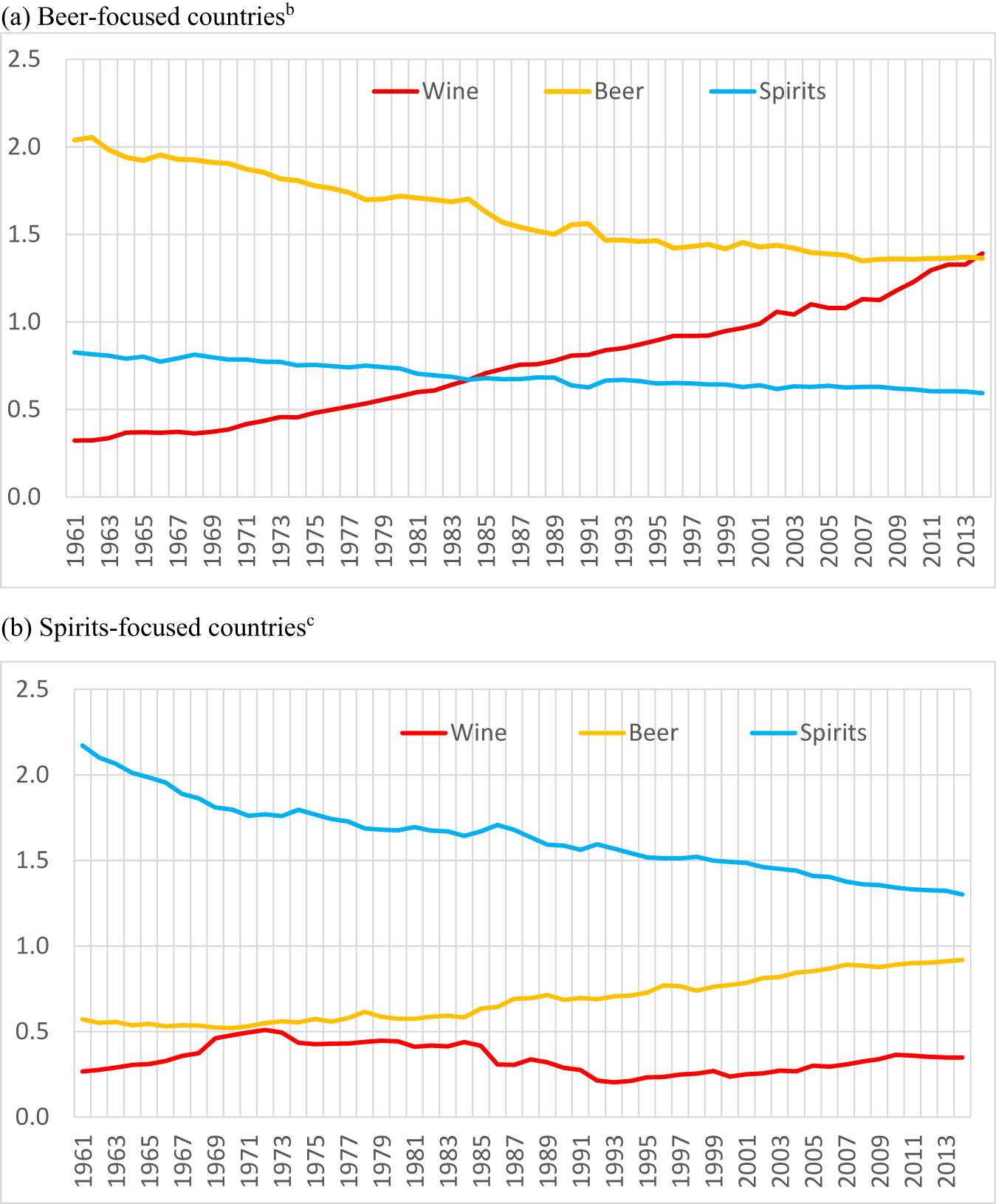
One way to capture that compositional change is with a consumption intensity index, defined as the fraction of wine, beer, or spirits consumption in total national alcohol consumption volume in country group i divided by the fraction for that same beverage in world total alcohol consumption. Figure 10(a) shows that the index dropped in beer-focused countries from more than 2 to less than 1.5 for beer, and rose from less than 0.4 to the same as beer (1.4) by 2014 (while their index for spirits fell slightly). Spirits-focused countries also converged somewhat toward the global mix by moving from spirits and toward beer, but without embracing wine (Figure 10(b)).

Figure 10.

Wine, beer, and spirits intensity of consumption indexes^a for beer-focused and spirits-focused countries, 1961–2014. (a) Beer-focused countries^b, (b) spirits-focused countries^c.

Figure 10 Long description

A showing a line graph with a legend listing Wine, Beer, Spirits. The horizontal axis shows years from 1961 to 2013. The vertical axis shows values from 0.0 to 2.5. Wine series coordinate pairs: (1961, 0.3), (1971, 0.4), (1981, 0.6), (1991, 0.8), (2001, 1.0), (2011, 1.3), (2013, 1.4). Beer series coordinate pairs: (1961, 2.0), (1971, 1.9), (1981, 1.7), (1991, 1.5), (2001, 1.4), (2011, 1.4), (2013, 1.4). Spirits series coordinate pairs: (1961, 0.8), (1971, 0.8), (1981, 0.7), (1991, 0.6), (2001, 0.6), (2011, 0.6), (2013, 0.6). B showing a line graph with a legend listing Wine, Beer, Spirits. The horizontal axis shows years from 1961 to 2013. The vertical axis shows values from 0.0 to 2.5. Wine series coordinate pairs: (1961, 0.3), (1971, 0.5), (1981, 0.4), (1991, 0.3), (2001, 0.3), (2011, 0.4), (2013, 0.4). Beer series coordinate pairs: (1961, 0.6), (1971, 0.5), (1981, 0.6), (1991, 0.7), (2001, 0.8), (2011, 0.9), (2013, 0.9). Spirits series coordinate pairs: (1961, 2.2), (1971, 1.8), (1981, 1.7), (1991, 1.6), (2001, 1.5), (2011, 1.3), (2013, 1.3).

aThe intensity index is defined as the fraction of wine, beer, or spirits consumption in total national alcohol consumption volume in country group i divided by the fraction for that same beverage in world total alcohol consumption. (The wine-focused countries as of 1961–64 are Algeria, Argentina, Bulgaria, Chile, Croatia, France, Georgia, Greece, Hungary, Italy, Moldova, Morocco, Portugal, Romania, Spain, Switzerland, Tunisia, Türkiye, Uruguay.)b The beer-focused countries as of 1961–64 are Australia, Austria, Belgium-Luxembourg, Canada, Denmark, Germany, Ireland, Malaysia, Mexico, Netherlands, New Zealand, Singapore, United Kingdom, United States, Other Eastern Europe, Other Latin America, Other African and Middle East.c The spirits-focused countries as of 1961–64 are Brazil, China, Finland, Hong Kong, India, Japan, Korea, Norway, Philippines, Russia, South Africa, Sweden, Taiwan, Thailand, Ukraine, Other Western Europe, Other Asia.Source: Updated from Holmes and Anderson (2017).

These trends and partial convergence toward the global average mix of alcohol consumption provide only partial support for the Stigler and Becker (Reference Stigler and Becker1977) theory that consumption bundles would become similar as per capita incomes converge. Furthermore, the data in Figure 9 only go up to 2014. The embracing of wine in beer-focused countries, most notably in Australasia, North America and north-western Europe, had not only come to an end before then but has since reversed considerably following the trend seen in the key wine-producing countries, thereby adding to wine's demise in volume terms (Figure 11).

Figure 11.

Wine consumption per capita in Australasia, North America and northwest Europe, 1960 to 2025 (liters). (a) Australasia and North America, (b) Northwest Europe.

Figure 11 Long description

A multi line time series graph with legend entries Australia, New Zealand, Canada, United States. Line styles: Australia shown as a solid line, New Zealand shown as a dotted line, Canada shown as a dashed line, United States shown as a dashed line. Horizontal axis label, 1960 to 2023. Vertical axis label, litres, with tick values from 0 to 25. Australia series coordinate pairs: (1960, 5), (1963, 5), (1966, 6), (1969, 8), (1972, 9), (1975, 12), (1978, 14), (1981, 18), (1984, 20), (1987, 21), (1990, 18), (1993, 19), (1996, 18), (1999, 20), (2002, 21), (2005, 22), (2008, 24), (2011, 24), (2014, 23), (2017, 22), (2020, 23), (2023, 19). New Zealand series coordinate pairs: (1960, 2), (1963, 2), (1966, 3), (1969, 4), (1972, 7), (1975, 9), (1978, 11), (1981, 14), (1984, 12), (1987, 15), (1990, 13), (1993, 15), (1996, 15), (1999, 16), (2002, 16), (2005, 20), (2008, 22), (2011, 21), (2014, 21), (2017, 20), (2020, 18), (2023, 15). Canada series coordinate pairs: (1960, 2), (1963, 2), (1966, 3), (1969, 4), (1972, 5), (1975, 6), (1978, 7), (1981, 9), (1984, 10), (1987, 10), (1990, 9), (1993, 8), (1996, 8), (1999, 8), (2002, 9), (2005, 12), (2008, 13), (2011, 14), (2014, 13), (2017, 14), (2020, 11), (2023, 7). United States series coordinate pairs: (1960, 3), (1963, 3), (1966, 3), (1969, 4), (1972, 5), (1975, 6), (1978, 7), (1981, 8), (1984, 9), (1987, 9), (1990, 7), (1993, 7), (1996, 7), (1999, 8), (2002, 8), (2005, 9), (2008, 9), (2011, 10), (2014, 10), (2017, 11), (2020, 10), (2023, 10). Key visible highs and lows from the listed points: Australia highest listed value 24 at 2008 and 2011, lowest listed value 5 at 1960 and 1963. New Zealand highest listed value 22 at 2008, lowest listed value 2 at 1960 and 1963. Canada highest listed value 14 at 2011 and 2017, lowest listed value 2 at 1960 and 1963. United States highest listed value 11 at 2017, lowest listed value 3 at 1960, 1963, 1966. The image B showing a multi line time series graph with legend entries Belgium Lux, Denmark, Netherlands, Sweden, United Kingdom. Line styles: Belgium Lux shown as a dashed line, Denmark shown as a dotted line, Netherlands shown as a solid line, Sweden shown as a dashed line, United Kingdom shown as a solid line. Horizontal axis label, 1960 to 2025. Vertical axis label, with tick values from 0 to 35. Belgium Lux series coordinate pairs: (1960, 8), (1965, 12), (1970, 15), (1975, 17), (1980, 20), (1985, 22), (1990, 23), (1995, 24), (2000, 23), (2005, 26), (2010, 25), (2015, 24), (2020, 22), (2025, 13). Denmark series coordinate pairs: (1960, 3), (1965, 4), (1970, 5), (1975, 10), (1980, 12), (1985, 18), (1990, 20), (1995, 25), (2000, 28), (2005, 32), (2010, 30), (2015, 28), (2020, 26), (2025, 23). Netherlands series coordinate pairs: (1960, 2), (1965, 3), (1970, 4), (1975, 9), (1980, 11), (1985, 17), (1990, 16), (1995, 18), (2000, 20), (2005, 22), (2010, 21), (2015, 20), (2020, 21), (2025, 16). Sweden series coordinate pairs: (1960, 3), (1965, 4), (1970, 5), (1975, 7), (1980, 9), (1985, 10), (1990, 11), (1995, 12), (2000, 13), (2005, 16), (2010, 24), (2015, 22), (2020, 20), (2025, 18). United Kingdom series coordinate pairs: (1960, 2), (1965, 2), (1970, 3), (1975, 5), (1980, 6), (1985, 9), (1990, 11), (1995, 12), (2000, 15), (2005, 22), (2010, 20), (2015, 19), (2020, 20), (2025, 18). Key visible highs and lows from the listed points: Belgium Lux highest listed value 26 at 2005, lowest listed value 8 at 1960. Denmark highest listed value 32 at 2005, lowest listed value 3 at 1960. Netherlands highest listed value 22 at 2005, lowest listed value 2 at 1960. Sweden highest listed value 24 at 2010, lowest listed value 3 at 1960. United Kingdom highest listed value 22 at 2005, lowest listed value 2 at 1960 and 1965. Purpose stated by the content of the two graphs: comparison of wine consumption per capita over time across the listed countries in the two regions.

Source: Anderson and Pinilla (2026).

One bright spot for wine in the 2010s was a rapid embracing of wine by spirits-focused China. However, that turned out to be short-lived and quickly reversed at the end of that decade, for reasons explained in Anderson (Reference Anderson2025b).Footnote ⁷

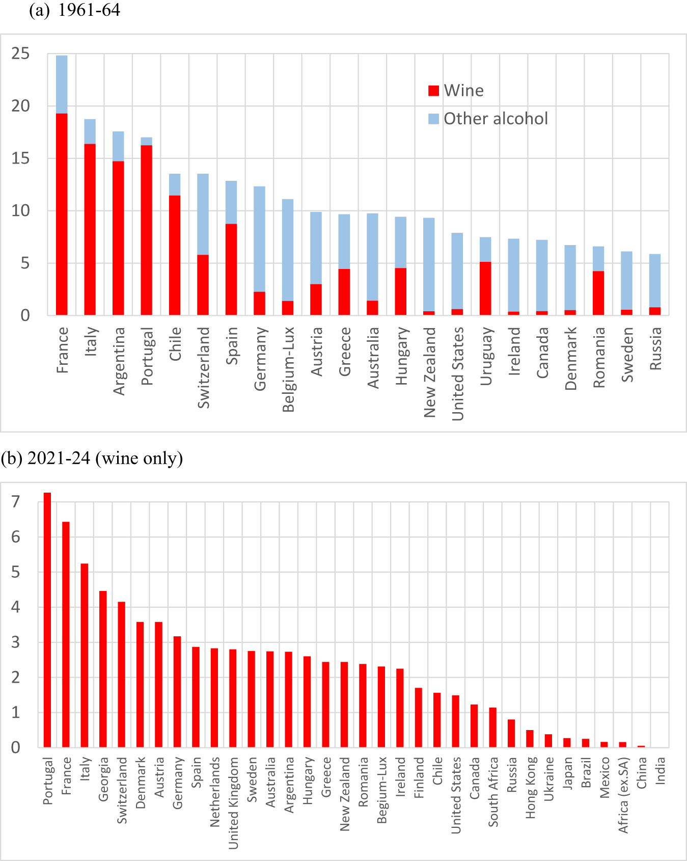
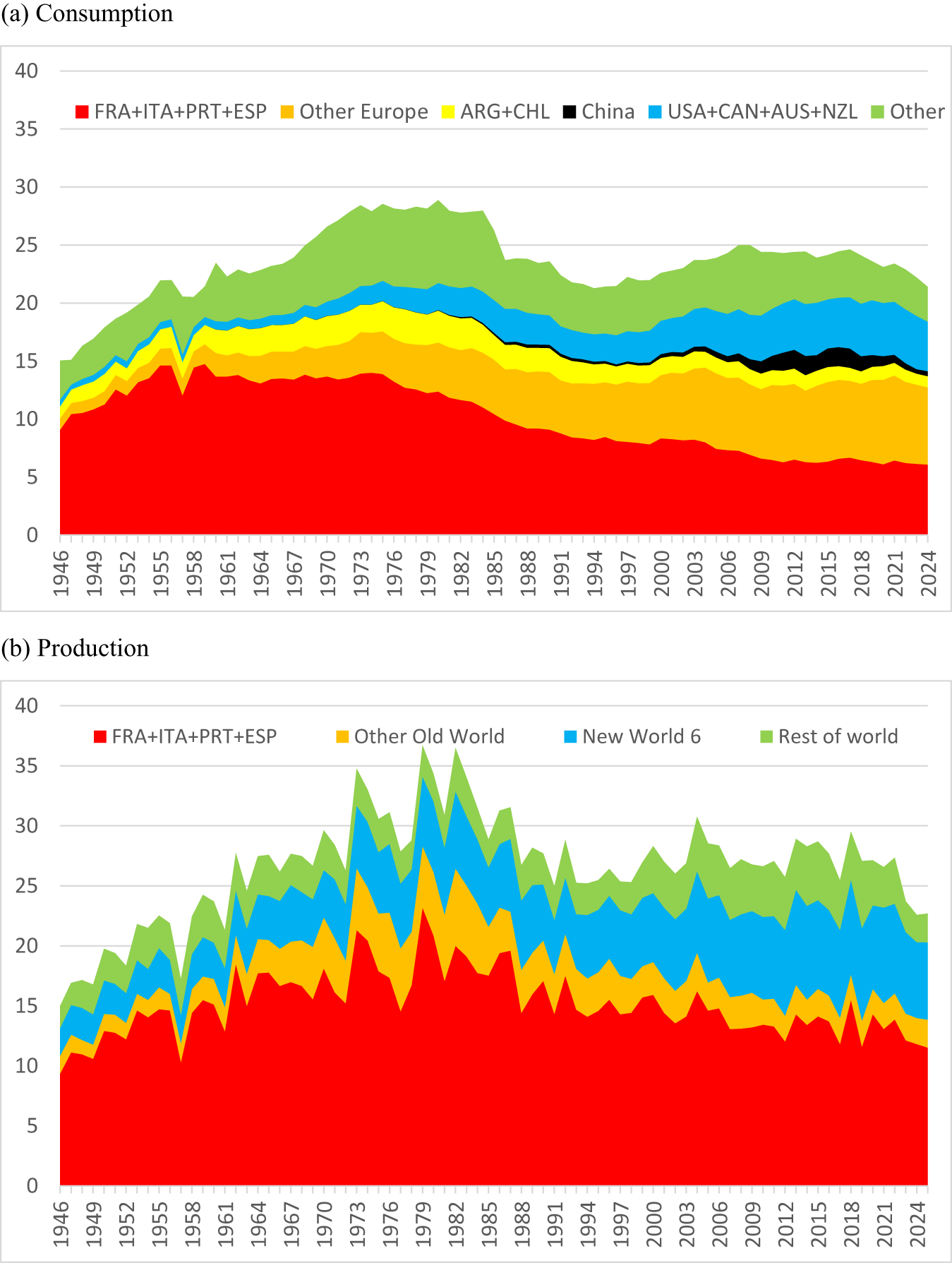
The enormity of European wine-based alcohol consumption in the first half of the 1960s is clear from Figure 12(a). The enormity also of that region's reduction in wine consumption by the first half of the 2020s can be seen by comparing Figures 12(a) and 12(b). Much of that reduction is in non-premium wine that was traditionally produced by large co-operative wineries. Even so, the top dozen wine-consuming countries remain European. Figure 13(a) provides a continuous picture since World War II of the changing importance of various regions in global wine consumption. Note that China's short-lived burst in the 2010s was barely enough to offset the continuing decline in wine consumption in Argentina and Chile.

Figure 12.

Volumes of wine and other alcohol consumption per adult, 1961–1964 and 2021–2024 (liters of alcohol). (a) 1961–1964, (b) 2021–2024 (wine only).

Figure 12 Long description

1961 dash 64. Legend labels, Wine and Other alcohol. The horizontal axis lists countries: France, Italy, Argentina, Portugal, Chile, Switzerland, Spain, Germany, Belgium dash Lux, Austria, Greece, Australia, Hungary, New Zealand, United States, Uruguay, Ireland, Canada, Denmark, Romania, Sweden, Russia. The vertical axis shows values from 0 to 25. Bars are stacked by category, with Wine as the lower segment and Other alcohol as the upper segment. The tallest total bar is France, reaching close to 25. Italy, Argentina and Portugal are the next highest totals, each below 20. Totals then step down across the remaining countries, with the smallest totals near 6 for Sweden and Russia. 2021 dash 24, wine only. The horizontal axis lists countries: Portugal, France, Italy, Germany, Switzerland, Denmark, Austria, Germany, Spain, Netherlands, United Kingdom, Sweden, Australia, Argentina, Hungary, Greece, New Zealand, Belgium dash Lux, Finland, Chile, United States, Canada, South Africa, Russia, Hong Kong, Ukraine, Israel, Brazil, Mexico, Africa dash USA, China, India. The vertical axis shows values from 0 to 7. A single bar series is shown. The highest bar is Portugal, slightly above 7. France is next, a little above 6. Italy is near 5 and Germany is between 4 and 5. Many countries in the middle are between 2 and 3. The smallest bars are near 0 for China and India. Both charts present country by country comparisons. The first chart separates Wine and Other alcohol within each country total and the second chart shows Wine only for a later period.

Source: Anderson and Pinilla (2026).

Figure 13.

Global volume of wine consumption by country/region, 1946–2025 (billion liters). (a) Consumption, (b) production.

Figure 13 Long description

The stacked area graph labeled, Consumption. The horizontal axis shows years from 1946 to 2024. The vertical axis shows values from 0 to 40. A legend lists, FRA plus ITA plus PRT plus ESP, Other Europe, ARG plus CHL, China, USA plus CAN plus AUS plus NZL, Other. The stacked areas form a combined total that rises from the mid teens near 1946 to the high twenties in the mid 1970s, then falls to the low twenties by the early 1990s, then rises to the mid twenties around the late 2000s to early 2010s and ends in the low twenties by 2024. The FRA plus ITA plus PRT plus ESP band is the largest early in the series, reaching the mid teens around the 1950s to 1960s, then declining to single digits by the 2000s and remaining near that level through 2024. Other Europe increases from a small band in the 1940s to a thicker band by the 1970s and remains a major portion through 2024. USA plus CAN plus AUS plus NZL grows gradually from a thin band early to a thicker band by the 2000s to 2020s. China appears as a thin band mainly in the 2000s to 2020s. ARG plus CHL remains a thin band throughout. Other forms a substantial upper band that increases into the 1970s, drops around the late 1980s to early 1990s, then varies through 2024. The stacked area graph labeled, Production. The horizontal axis shows years from 1946 to 2024. The vertical axis shows values from 0 to 40. A legend lists, FRA plus ITA plus PRT plus ESP, Other Old World, New World 6, Rest of world. The stacked areas form a combined total that rises from the mid teens near 1946 to the mid to high twenties by the 1960s, reaches peaks in the mid to high thirties around the late 1970s to early 1980s, then declines to the mid twenties by the early 1990s and varies around the mid to high twenties through the 2000s to 2024. The FRA plus ITA plus PRT plus ESP band is the largest throughout, rising from around 10 near 1946 to around 20 in the 1970s to early 1980s, then declining to the mid teens by the 2000s to 2020s. Other Old World forms a mid level band that is thicker around the 1970s to 1980s and thinner after the 1990s. New World 6 increases from a thin band early to a thicker band after the 1990s and remains substantial through 2024. Rest of world forms the top band and varies in thickness across the timeline.

a“New World 6” is Argentina, Australia, Chile, New Zealand, South Africa, and the United States.Source: Anderson and Pinilla (2026), based on OIV statistics.

b. Why the move away from reds

The declining interest in red wines may be partly just a fashion change that could reverse in future decades. It may also be partly because global warming has had the undesirable effect of raising alcohol levels more in red wines than in white wines, rosé and sparkling wines. Two further factors may be the gradually declining influence this century of wine critic Robert Parker, who had a strong preference for high-alcohol reds, and more recently the shrinkage of (what was 90% red) wine consumption in China. A further contributor is a change in the general perception about red wine's influence on human health: it was widely accepted up until a decade or so ago that moderate consumption of red wine contributed to healthy aging, but that has been thrown into doubt by anti-alcohol lobbies pointing to studies disputing that view.

c. Why the growth in new world wine production and exports

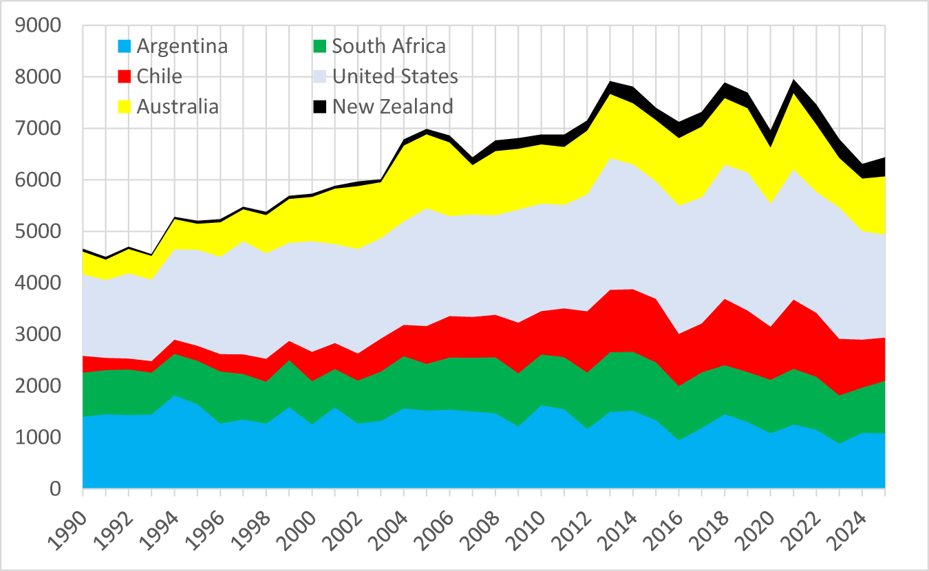
While European producers were still struggling to reduce their non-premium wine production at the pace their consumption of it was declining, in the two decades to 2012 the New World nearly doubled its wine production (Figure 14). In fact, its output rose 2.4 times if one excludes Argentina and South Africa, whose combined output has trended slightly downward since 1990.

Figure 14.

Volume of wine production in New World countries, 1990–2025 (million liters).

Figure 14 Long description

The vertical axis shows 0 to 9000. The horizontal axis shows 1990 to 2025. Legend: Argentina, Chile, Australia, South Africa, United States, New Zealand. Stacked layers represent each country and the top edge represents the total. Total is about 4500 in 1990, rises to about 7000 by 2005, peaks near 8000 around 2013 to 2014 and again around 2021 to 2022, then declines to about 6300 to 6500 by 2025. The United States layer is the largest for most years, rising from about 1500 in 1990 to about 2500 to 2700 around 2013 to 2014, then about 2000 to 2300 by 2025. Argentina is about 1400 in 1990, about 1600 around 2005 and about 1000 to 1100 by 2025. South Africa is about 800 in 1990, about 900 to 1000 around 2005 to 2015 and about 1000 by 2025. Chile rises from about 300 in 1990 to about 1200 to 1300 around 2013 to 2014, then about 900 to 1000 by 2025. Australia rises from about 300 to 400 in 1990 to about 1200 to 1300 around 2005 to 2007, then about 800 to 900 by 2025. New Zealand remains the smallest layer, about 100 in 1990 and about 300 to 400 by 2025.

Source: Anderson and Pinilla (2026), based on OIV statistics.

The majority of that increase in New World production was exported, since those countries’ domestic consumption has increased by only one-quarter since 1990. In the 1980s, exports accounted for less than 2% of their output but, by the 2010s, that share averaged 40%. The dramatic increase in their international competitiveness is revealed in the rapid rise in their shares of global wine exports, shown in Figure 6.

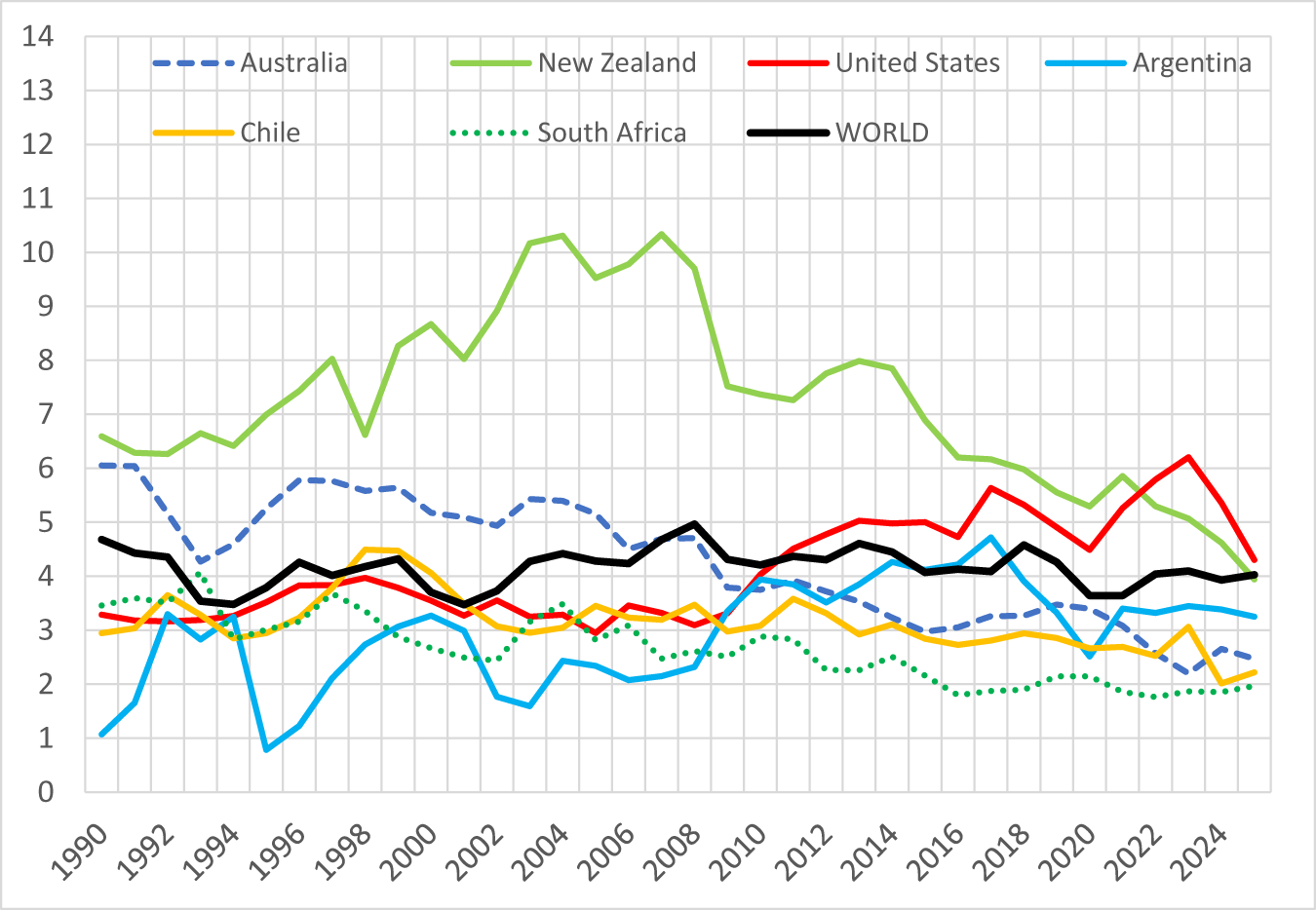
Most of that expanded production in New World countries is what IWSR would define as non-premium (retailing at less than US$10 per 75cl bottle or equivalent), judging by the average price of those countries’ exports. Apart from the small volumes from New Zealand, the only countries whose average export price exceeded the world average were Australia up to 2006 and the United States from 2011 (Figure 15). True, the average share of those exports transported in bulk has risen very considerably this century while that share has changed little for the world as a whole (Table 1). But even if a more appropriate indicator of wine quality were to be available, it is likely to show that most New World production falls into the non-premium (particularly branded commodity) wine category.

Figure 15.

Real price of wine exports of New World countries and the world, 1990–2025 (US$ per liter, inflated to 2025 dollars using the U.S. CPI).

Figure 15 Long description

Real price of wine exports per litre, inflated to 2025 dollars using the US CPI. The horizontal axis represents years from 1990 to 2024. The vertical axis represents price in dollars per litre, ranging from 0 to 14. Lines represent Australia, New Zealand, United States, Argentina, Chile, South Africa and WORLD. Australia shows a decline from 6 dollars in 1990 to 2.6 dollars in 2024. New Zealand peaks at 10.3 dollars in 2004, declining to 4.2 dollars in 2024. The United States rises from 3.3 dollars in 1990 to a peak of 6.2 dollars in 2023, ending at 4.3 dollars in 2024. Argentina fluctuates, peaking at 4.7 dollars in 2017, ending at 3.2 dollars in 2024. Chile shows a steady decline from 3 dollars in 1990 to 2.2 dollars in 2024. South Africa decreases from 3.5 dollars in 1990 to 1.9 dollars in 2024. WORLD average fluctuates around 4 dollars. New Zealand′s line is solid green, Australia is dashed blue, United States is solid red, Argentina is solid light blue, Chile is solid yellow, South Africa is dotted green and WORLD is solid black. The graph highlights New Zealand′s early 2000s highs and Australia′s long decline. It shows relative pricing trends across exporters compared to the world average.

Source: Anderson and Pinilla (2026), based on UN COMTRADE data.

Table 1.

Shares of wine exports transported in bulk containers, New World countries, 2000, 2012, and 2024 (%)

Table 1 Long description

Percent shares are given for wine exports transported in bulk containers, split into volume and value, for 2000, 2012, and 2024. Argentina volume is 24, 45, and 21; value is 10, 16, and 6. Australia volume is 12, 53, and 66; value is 4, 22, and 21. Chile volume is 29, 39, and 39; value is 13, 19, and 16. New Zealand volume is 2, 30, and 54; value is 1, 15, and 29. South Africa volume is 33, 64, and 54; value is 12, 36, and 26. United States volume is 13, 43, and 63; value is 7, 17, and 24. World volume is 35, 37, and 37; value is 9, 11, and 9.

Source: OIV (2026 and earlier).

Such an expansion of New World production in the face of declining global consumption of non-premium wine necessarily puts downward pressure on the average price of the world's non-premium wine and hence winegrapes (Figure 1(b)).

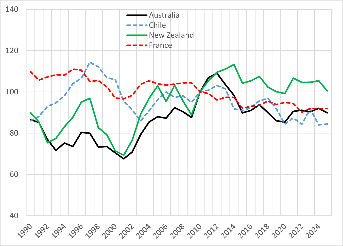
There are several key reasons why the New World was able to expand its production for export despite it depressing the world prices of non-premium wine in terms of U.S. dollars. First, southern hemisphere commodity exporting countries saw their real exchange rates depreciate very considerably from the mid-1990s to the early 2000s (or at the end of 2001 in the case of Argentina, when its currency was moved away from parity with the U.S. dollar), as shown in Figure 16. Those depreciations raised their wine export prices and thus their domestic winegrape prices in local currency terms in the 1990s, as evidenced in Figure 8.

Figure 16.

Real exchange rate indexes,^a New World countries, 1990–2025 (2010 = 100).

aA fall in the index in this figure represents a real depreciation.Source: World Bank (2026a).

Second, four technology revolutions overlapped: the ICT one that lowered the cost of information and communication flows across national borders, the ocean transport revolution (containerization) that reduced the disadvantage of being further from the UK, United States, and other key markets than Old World vignerons, the supermarket revolution and associated deregulation of liquor retailing in the UK, and the revolution in tertiary education of viticulturalists and enologists and the flow-on that had to higher-quality grape and wine R&D, particularly in the United States and Australia before it spread elsewhere.

Third, large wineries in those New World countries consolidated through acquisitions and mergers to form what eventually became huge multinational corporations capable of negotiating effectively with the huge supermarkets in the UK and elsewhere. Their large size enabled them to draw promptly on new technologies and develop brands of fault-free commercial wines that readily attracted newcomer consumers because of their consistency from year to year, drinkability when still young, and perceived good value for money. Those corporations were able to expand production rapidly because they had the cash to plant new vineyards as well as to offer initially attractive long-term contracts to independent growers. In Australia, that was made all the more affordable because of lucrative government tax incentives for investors, and was encouraged by a 30-year strategic plan the industry launched in 1996 (Anderson, Reference Anderson2018, Reference Anderson2024).

And fourth, competition from the Old World was reduced by several food-safety scares, notably scandals involving additives to Austrian wines (diethylene glycol) in 1985 and to Italian wines (methanol) in 1986, and then the Chernobyl nuclear plant disaster in April 1986.

Despite the New World's vineyard expansion, the global winegrape-bearing area has been declining, falling between 1990 and 2023 from 5.4 to 4.5 million hectares (Anderson, Nelgen, Puga, et al., Reference Anderson, Nelgen and Puga2026). Numerous informed commentators have suggested a similar-sized reduction is needed now (e.g., Joseph, Reference Joseph2026). It is thus sobering to note the earlier one-sixth reduction took one-third of a century.

d. Why the global surplus

Those real exchange rate depreciations of the 1990s reversed in the 2000s but—as happens for perennial crops—producers were slow to begin reducing their output. Adjustment to bearing areas was delayed further as those currencies depreciated again in the 2010s (Figure 14) and as China unexpectedly became a significant wine importer, mostly of still reds. The equally unexpected fall in China's demand from the late 2010s then further added to the necessity to reduce the global surplus, particularly of red wine.

Then the COVID-19 pandemic hit in the early 2020s. It raised the cost of ocean transport enormously, such that the fob export price of southern hemisphere bulk wine, which normally would have been destined for Europe and North America, was driven down to almost zero. That transport crisis eased in the years that followed, but meanwhile more vintages of wine had accumulated in tanks. Distillers too were overwhelmed by the excess supply of unwanted wine, to the point where they could not pay enough even to cover the cost of trucking surplus wine to their distilling plants (except in those parts of the EU where government subsidies were again being offered recently to encourage such disposal). At the time of writing this article (the beginning of the northern hemisphere's 2026 vintage), the surplus still hanging over the market continues to depress winegrape price expectations.