









1 Introduction
Differential heating applied at the horizontal surface of a basin of water results in a convective circulation, termed ‘horizontal convection’ (Rossby Reference Rossby1965, Reference Rossby1998; Hughes & Griffiths Reference Hughes and Griffiths2008). The motion involves a stratified diffusive boundary layer at the surface and an overturning circulation extending the length of the basin between the coldest and hottest parts of the surface. At large geophysical scales Coriolis accelerations resulting from planetary rotation are expected to have a strong influence, and several flow regimes have been identified in the case of a rotating annulus with a radial temperature gradient applied to the base (Hignett, Ibbetson & Killworth Reference Hignett, Ibbetson and Killworth1981). In particular, under strong rotation the transport is controlled by geostrophic balance in the thermal boundary layer. In the case of a rotating rectangular box, side wall boundary layers tend to break the geostrophic constraint and allow greater transport. However, experimental results with heating and cooling applied to regions of the base at opposite ends of a box are again somewhat consistent with the geostrophic boundary layer scaling (Park & Whitehead Reference Park and Whitehead1999). Work on the rotating annulus or re-entrant channel models has considered stability of the flow and the mechanical energy budget (Quon Reference Quon1987; Colin de Verdière Reference Colin de Verdière1988; Winton Reference Winton1996; Barkan, Winters & Llewellyn Smith Reference Barkan, Winters and Llewellyn Smith2013; Sheard, Hussam & Tsai Reference Sheard, Hussam and Tsai2016) and potential vorticity dynamics (Zhang et al. Reference Zhang, Chen, Zhang and Wang2016).
Existing analyses, laboratory experiments and simulations of rotating horizontal convection have considered only conditions at which the thermal boundary layer is laminar, excepting recent direct numerical simulations for a rectangular basin (Vreugdenhil, Gayen & Griffiths Reference Vreugdenhil, Gayen and Griffiths2016). Those simulations, with a temperature difference applied over two halves of the base, showed flow controlled by a turbulent thermal boundary layer at large Rayleigh numbers,
 $Ra>10^{11}$
, in line with results for the non-rotating case (Mullarney, Griffiths & Hughes Reference Mullarney, Griffiths and Hughes2004; Hughes et al.
Reference Hughes, Griffiths, Mullarney and Peterson2007; Gayen, Griffiths & Hughes Reference Gayen, Griffiths and Hughes2014). They also showed that the vertical heat transport into the interior takes place in columnar vortices over some of the area of destabilising boundary flux. The turbulence has implications for the mechanisms for dissipation, and the columnar vortices potentially imply additional dynamical regimes in which the heat transport is not controlled by the boundary layer. Here we report laboratory experiments at similarly large Rayleigh numbers.
Early conceptual formulations of ocean circulation described the subtropical thermocline and meridional overturning in simple form, for a basin such as the North Atlantic, in terms of a geostrophic balance within the quasi-horizontal and strongly stratified upper boundary layer. This was coupled to upwelling of cold water through the thermocline and matching downward turbulent diffusion of heat (Robinson & Stommel Reference Robinson and Stommel1959; Robinson Reference Robinson1960; Bryan Reference Bryan1987; Winton Reference Winton1996; Park & Bryan Reference Park and Bryan2000) in order to find a simple scaling for the transport as a function of the surface temperature difference and vertical diffusivity. The scaling is similar to that predicted in the geostrophic boundary layer regime of horizontal convection in a rotating annulus. The closure of the circulation through sinking of cold water into the abyssal ocean at high latitudes was not included, and this part of the flow has been treated somewhat separately in other simple theories.
The sinking leg of the ocean overturning occurs at high latitudes, where the sea surface buoyancy flux is destabilising and produces areas of deep convection, which cools the water to depths of 1000–2000 m. These areas of convection, termed ‘chimneys’, have been analysed in terms of regional inflow near the surface and outflow at depths constrained by geostrophic balance, but with the heat transport enhanced by baroclinic instability. The chimneys are hundreds of kilometres across, within which vertical convection in the form of cyclonic plumes at the scale of 1–2 km is predicted to be three-dimensional, inertially controlled and free of geostrophic constraints (Jones & Marshall Reference Jones and Marshall1993; Maxworthy & Narimousa Reference Maxworthy and Narimousa1994; Send & Marshall Reference Send and Marshall1995; Marshall & Schott Reference Marshall and Schott1999). Assuming an inviscid flow forced by a sustained buoyancy flux
 $B$
out of the sea surface it was argued that the convection depends on the convective Rossby number
 $Ro^{\ast }=B^{1/2}/f^{3/2}H^{\ast }$
, where
 $f$
is the Coriolis parameter and
 $H^{\ast }$
is the depth of convection. For
 $Ro^{\ast }>0.078$
experiments suggest that rotation is unimportant,
 $H^{\ast }$
constrains the length scale of convective eddies, and the convection velocity scales as
 $(BH^{\ast })^{1/3}$
(Deardorff Reference Deardorff and Weil1985; Jones & Marshall Reference Jones and Marshall1993). For
 $Ro^{\ast }<0.078$
rotation strongly affects the convective plumes, setting their length scale
 $L^{\ast }\sim (B/f^{3})^{1/2}$
and velocity scale
 $U^{\ast }\sim (B/f)^{1/2}$
, independent of the depth. The conditions for ocean convection were placed in the non-rotating convection regime at
 $Ro^{\ast }>0.078$
(Klinger & Marshall Reference Klinger and Marshall1995). The deep convection relates to the sinking leg of the overturning in that it cools a large fraction of the water column and produces dense water, which then sinks to larger depths as dense currents on the sloping bottom. However, these studies do not show how deep convection is coupled to a large-scale overturning circulation and whether it controls transport. Although the circulation involves many other factors, including wind stress, Sverdrup flow, potential vorticity dynamics and the bathymetry, the buoyancy forcing is an important component (Saenz et al.
Reference Saenz, Hogg, Hughes and Griffiths2012). In this paper we examine the dynamics of a buoyancy-driven circulation in a simple rectangular basin.
Boundary layer analysis of non-rotating horizontal convection leads to scaling that is robust to the strength of the buoyancy forcing. A horizontal momentum balance between buoyancy and viscous stress, coupled to an advection–diffusion balance in the vertical (Rossby Reference Rossby1965) gives the non-dimensionalised heat transport, or Nusselt number,
 $Nu\sim Ra^{1/5}$
(where
 $Ra$
is the Rayleigh number based on the applied temperature difference and the horizontal scale over which the temperature difference is applied). This result has been supported by experimental results and numerical simulations at
 $Ra\leqslant 10^{9}$
, a range of Prandtl numbers and various imposed temperature distributions along the base (Rossby Reference Rossby1998; Wang & Huang Reference Wang and Huang2005; Gayen et al.
Reference Gayen, Griffiths and Hughes2014). At much larger Rayleigh numbers (
 $Ra>10^{11}$
), using piecewise uniform boundary conditions of imposed heat flux on the base of a long box, experiments show that much of the heated part of the boundary layer is turbulent as a result of small-scale convection (Mullarney et al.
Reference Mullarney, Griffiths and Hughes2004; Stewart, Hughes & Griffiths Reference Stewart, Hughes and Griffiths2011). Direct numerical simulations (DNS) of the same arrangement but with imposed temperature difference show that the flow is governed by a turbulent Reynolds stress (Gayen et al.
Reference Gayen, Griffiths and Hughes2014). The results again give
 $Nu\sim Ra^{1/5}$
, as predicted by scaling theory based on an inertial–buoyancy balance in the boundary layer. At the intermediate Rayleigh numbers there is a stronger dependence of
 $Ra$
due to a sequence of stability transitions, and therefore no dynamical similarity regime can be applied.
Analysis of horizontal convection in a rotating annulus also has assumed boundary layer control and laminar flow. The effects of rotation were delineated in terms of the ratio
 $Q$
of the thermal boundary layer thickness to Ekman layer thickness (Hignett et al.
Reference Hignett, Ibbetson and Killworth1981). When rotation is strong the Ekman layer is thin, leaving the bulk of the thermal boundary layer decoupled from boundary stress and governed by a geostrophic balance, with velocities
 $U\sim (\unicode[STIX]{x1D705}/L)(RaE)^{2/3}$
and boundary layer thickness
 $\unicode[STIX]{x1D6FF}\sim L(RaE)^{-1/3}$
, where
 $L$
is the basin length scale,
 $E$
is the Ekman number and
 $\unicode[STIX]{x1D705}$
is the molecular diffusivity. Although an alternative theory includes a frictional term that results in scaling more strongly dependent on Coriolis parameter (Stern Reference Stern1975), the laboratory experiments with a rectangular basin (adjusted for an imposed heat flux boundary condition and corrected for Ekman transport) gave results consistent with the frictionless case (Park & Whitehead Reference Park and Whitehead1999). The experiments also showed large-scale horizontal gyre circulation that extended throughout the depth. Physically, the flow in the direction of the temperature gradient is inhibited by geostrophic balance, leading to smaller velocities, thicker boundary layer and smaller heat transport for larger rotation rate or smaller buoyancy forcing. Numerical modelling of horizontal convection in a rotating re-entrant channel with imposed flux showed that heat transport is primarily by baroclinic eddies (Barkan et al.
Reference Barkan, Winters and Llewellyn Smith2013), which was also found for the axisymmetric case with side wall forcing (Read Reference Read1986, Reference Read2003). For very large Rayleigh numbers, scaling analysis indicates that it is appropriate to use an inviscid parameter
 $QPr$
(where
 $Pr$
is the Prandtl number) in place of
 $Q$
(Vreugdenhil et al.
Reference Vreugdenhil, Gayen and Griffiths2016), and DNS for turbulent conditions has provided the condition (
 $QPr\approx 10$
) for the transition between non-rotating and geostrophic boundary layer regimes. The DNS also showed that strong rotation does not affect the total dissipation of kinetic energy in the flow until the conditions are so extreme that Coriolis accelerations change the turbulent dissipation at scales smaller than the boundary layer thickness. Consistent with previous work (Sheard et al.
Reference Sheard, Hussam and Tsai2016) a transition to a conduction-dominated regime was identified at extremely rapid rotation.
Here we report laboratory experiments with rotation, using a closed rectangular basin and Rayleigh numbers large enough to ensure turbulent inertial–buoyancy regimes in both the non-rotating and geostrophic regimes. A heat flux boundary condition is used, rather than an imposed temperature difference, as the imposed uniform flux case avoids complicated in situ measurements of heat flux and its distribution over the heated area, and hence allows more accurate measurements of the Nusselt number. Perhaps more significantly, the case of imposed temperature difference with large Rayleigh number can be studied by direct numerical simulation, whereas the imposed heat flux case (for which the thermal equilibration times are longer than for the case with an imposed temperature difference by a factor of four) has proved too demanding for current supercomputer capacities (Gayen et al. Reference Gayen, Griffiths, Hughes and Saenz2013a , Reference Gayen, Griffiths and Hughes2014; Griffiths, Hughes & Gayen Reference Griffiths, Hughes and Gayen2013; Vreugdenhil et al. Reference Vreugdenhil, Gayen and Griffiths2016). As insights from both boundary conditions are likely to be relevant to the oceans, the absence of computer simulations with imposed flux motivate these experiments. In § 2 scaling analyses are presented for non-rotating, geostrophic boundary layer and ‘chimney convection’ regimes, and it is argued that the convective Rossby number based on the imposed buoyancy flux is the most appropriate parameter to use in describing the changes in flow dynamics from weak rotation to geostrophic regimes. The apparatus and methods are outlined in § 3, and tests of the approach to thermal equilibrium and the equilibration time scale are shown in § 4. Observations from flow visualisation are given in § 5, while § 6 reports measurements of the boundary layer flow with comparison to the scaling theories, § 7 presents data for the velocity and overturning transport in the bulk of the fluid, and § 8 gives information on the frequency spectra of temperature fluctuations. The results are discussed in § 9 with conclusions in § 10.
2 Theoretical analysis
We consider the flow in a rotating rectangular basin having length
 $L$
, width
 $W$
and height
 $H$
, with all boundaries no slip. All boundaries excepting the base are insulating. The base has a uniform heat flux per unit area
 $F$
, corresponding to a uniform buoyancy flux per unit area
 $B$
, applied over half its length (figure 1). The other half of the base is held at a uniform temperature
 $T_{c}$
. The temperatures in the flow besides those at the cooled boundary are free to adjust until a thermal equilibrium state is reached, at which time the (time-averaged) heat withdrawn by the cooled section of the base must be equal to the (constant) heat input.
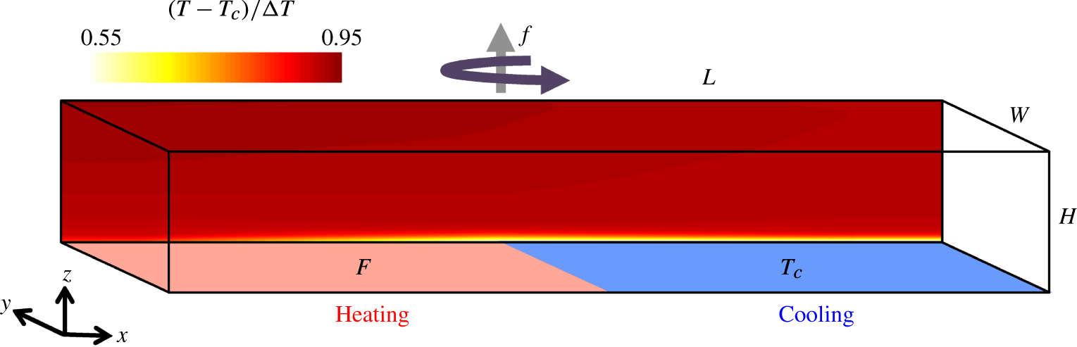
The laboratory arrangement with heating as a uniform flux imposed through half of the base and cooling imposed as a uniform temperature over the other half. The back-drop shows the measured time-averaged (over 12 h) temperature in the flow at
 $y/W=0.67$
for
 $Ra_{F}=6.5\times 10^{14}$
and
 $f=0.4~\text{s}^{-1}$
(
 $Ro=5.6\times 10^{-3}$
).
The governing parameters are the flux Rayleigh number, the Prandtl number, the Ekman number and the vertical and horizontal aspect ratios, respectively
 $$\begin{eqnarray}Ra_{F}=\frac{BL^{4}}{\unicode[STIX]{x1D708}\unicode[STIX]{x1D705}^{2}},\quad Pr=\frac{\unicode[STIX]{x1D708}}{\unicode[STIX]{x1D705}},\quad E=\frac{\unicode[STIX]{x1D708}}{fL^{2}},\quad A=\frac{H}{L},\quad A_{y}=\frac{W}{L},\end{eqnarray}$$
where
 $\unicode[STIX]{x1D708}$
is molecular viscosity,
 $\unicode[STIX]{x1D705}$
the thermal diffusion coefficient of the fluid,
 $f$
is the Coriolis parameter (assumed uniform here) and where all parameters involving length scale are defined in terms of the forcing length scale
 $L$
. Assuming a linear equation of state
 $B=g\unicode[STIX]{x1D6FC}F/\unicode[STIX]{x1D70C}_{0}c_{p}$
where
 $g$
is the gravitational acceleration,
 $\unicode[STIX]{x1D6FC}$
is the thermal expansion coefficient,
 $\unicode[STIX]{x1D70C}_{0}$
is a reference density and
 $c_{p}$
is the specific heat capacity. This assumption is a simplifying convenience that ensures that conservation of heat implies conservation of buoyancy and that there is zero net buoyancy flux in a thermally equilibrated state.
The Nusselt number, measuring the convective heat transport relative to purely conductive transfer, is defined as
 $$\begin{eqnarray}Nu=\frac{BL}{\unicode[STIX]{x1D705}g\unicode[STIX]{x1D6FC}\unicode[STIX]{x0394}T},\end{eqnarray}$$
where
 $\unicode[STIX]{x0394}T=T_{h}-T_{c}$
is the temperature difference between the measured highest temperatures in the heated base and the imposed temperature of the cooling boundary. An alternative estimate based on the highest temperature measured at mid-depth and the cooling boundary temperature gave Nusselt number values that were not significantly different. Thus the Nusselt number serves as a dimensionless expression of the temperature difference maintained by the flow in providing the buoyancy forces necessary to achieve the imposed heat transport. The flux Rayleigh number is related to the Rayleigh number (
 $Ra=g\unicode[STIX]{x1D6FC}\unicode[STIX]{x0394}TL^{3}/\unicode[STIX]{x1D708}\unicode[STIX]{x1D705}$
) based on the temperature difference, by the expression
 $Ra_{F}=NuRa$
.
In this paper we consider only very large Rayleigh numbers (by which we mean
 $Ra>10^{11}$
or
 $Ra_{F}>10^{13}$
, for the particular distribution of heating and cooling considered here) and
 $Pr\approx 4{-}5$
, rather than the moderate Rayleigh numbers (
 $Ra<10^{10}$
or
 $Ra_{F}<10^{12}$
) examined in most studies and for which the flow is viscous (Rossby Reference Rossby1965, Reference Rossby1998; Paparella & Young Reference Paparella and Young2002; Wang & Huang Reference Wang and Huang2005). Non-rotating experiments in a box like that described above and with
 $Ra_{F}=O(10^{12}{-}10^{14})$
(Mullarney et al.
Reference Mullarney, Griffiths and Hughes2004; Stewart et al.
Reference Stewart, Hughes and Griffiths2011) showed that a stably stratified, cold boundary layer is maintained adjacent to the cooled boundary. The cold water flows horizontally in a boundary layer having thickness
 $0.05{-}0.1H$
, to the heated region, where it warms from the bottom and spatial instability leads to streamwise rolls near the leading edge of the heated region of the base, developing into small-scale turbulent convection in the boundary layer after a short distance. The small-scale convection forms a spatially developing convectively mixed layer, capped over most of the length of the heated area by the stable density gradient in the remaining upper region of the cold boundary layer. The thermal boundary layer feeds into an end wall plume that penetrates the depth of the box and forms a lateral outflow along the top of the box. Elsewhere in the interior (the bulk of the fluid) the average flow is a slow downward motion back into the cold boundary layer. When the box is rotating, the flow involves more complicated horizontal circulations. The Coriolis accelerations will tend to inhibit flow and heat transport along the box, while the side boundaries will break that constraint and allow a greater transport than expected in an annulus.
Predictions for the flow dynamics can be obtained by scaling analysis, working from the Navier–Stokes momentum equation in a rotating coordinate frame in the incompressible and Boussinesq approximation, along with conservation of mass and heat:
 $$\begin{eqnarray}Pr^{-1}\left(\frac{\text{D}\hat{\boldsymbol{u}}}{\text{D}\hat{t}}+\unicode[STIX]{x1D735}\hat{p}\right)=\unicode[STIX]{x1D6FB}^{2}\hat{\boldsymbol{u}}+Ra_{F}\hat{T}\boldsymbol{k}-E^{-1}\boldsymbol{k}\times \hat{\boldsymbol{u}},\end{eqnarray}$$
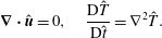 $$\begin{eqnarray}\unicode[STIX]{x1D735}\boldsymbol{\cdot }\hat{\boldsymbol{u}}=0,\quad \frac{\text{D}\hat{T}}{\text{D}\hat{t}}=\unicode[STIX]{x1D6FB}^{2}\hat{T}.\end{eqnarray}$$
The bold font signifies vectors, the hats indicate dimensionless variables,
 $\hat{\boldsymbol{u}}=(\hat{u} ,\hat{v},{\hat{w}})$
is the velocity,
 $\hat{t}$
is time,
 $\hat{p}$
is the pressure deviation from the hydrostatic,
 $\hat{T}=T(\unicode[STIX]{x1D705}g\unicode[STIX]{x1D6FC}/BL)$
is the temperature deviation and
 $\boldsymbol{k}$
is the unit upward vector. The variables have been non-dimensionalised by length
 $L$
, time
 $L^{2}/\unicode[STIX]{x1D705}$
, mass
 $\unicode[STIX]{x1D70C}_{0}L^{3}$
and a scale
 $BL/\unicode[STIX]{x1D705}g\unicode[STIX]{x1D6FC}$
for the temperature difference.
2.1 Non-rotating scaling
The non-rotating scaling for very large Rayleigh numbers is briefly reviewed here for the purpose of comparison with rotating cases. After neglecting rotation and eliminating the pressure in
 $x$
and
 $z$
components of the momentum equation (2.3) an inertial–buoyancy balance gives
 $$\begin{eqnarray}\frac{\unicode[STIX]{x2202}}{\unicode[STIX]{x2202}z}(u\boldsymbol{\cdot }\unicode[STIX]{x1D735}u)\sim \frac{\unicode[STIX]{x2202}}{\unicode[STIX]{x2202}x}g\unicode[STIX]{x1D6FC}T.\end{eqnarray}$$
Taking vertical gradients in the boundary layer much larger than horizontal gradients and scaling terms in (2.5) with
 $U$
for horizontal velocity,
 $\unicode[STIX]{x1D6FF}_{m}$
for the turbulent momentum boundary layer thickness,
 $L$
for horizontal length and
 $\unicode[STIX]{x0394}T$
for temperature, this becomes
 $$\begin{eqnarray}U^{2}/\unicode[STIX]{x1D6FF}_{m}L\sim g\unicode[STIX]{x1D6FC}\unicode[STIX]{x0394}T/L.\end{eqnarray}$$
The viscous scaling of Rossby (Reference Rossby1965, Reference Rossby1998) was based on momentum and thermal boundary layers of similar thickness, and we argue that the same result holds for the turbulent scaling. The stable thermal boundary layer is sustained by diffusion over the cooled region, which sets up a horizontal temperature gradient and leads to advection in the boundary layer towards the heated region of the boundary. In the turbulent case the drag is dominated by Reynolds stress produced by the small-scale convective turbulence (Gayen et al.
Reference Gayen, Griffiths, Hughes and Saenz2013a
, Reference Gayen, Griffiths and Hughes2014), and this is confined to a layer within, or beneath, the stably stratified thermal boundary layer, growing to the full thermal boundary layer thickness toward the end of the box. Hence the momentum boundary layer is within the thermal boundary layer and follows the same scaling,
 $\unicode[STIX]{x1D6FF}\sim \unicode[STIX]{x1D6FF}_{m}$
. This is strongly supported for the inertial-buoyancy regime by DNS and large eddy simulations (LES) in the ranges [
 $Ra\approx 10^{12}$
,
 $0.05\leqslant Pr\leqslant 5$
] and [
 $10^{12}<Ra<10^{15}$
,
 $Pr=5$
] respectively (Gayen et al.
Reference Gayen, Griffiths and Hughes2014). Matching thermal diffusion in the vertical within the thermal boundary layer against vertical advection of heat (again as in the previous viscous scaling), and matching the vertical mass transport to the horizontal transport by continuity, the heat equation (2.4) gives
 $$\begin{eqnarray}U/L\sim \overline{w}/\unicode[STIX]{x1D6FF}\sim \unicode[STIX]{x1D705}/\unicode[STIX]{x1D6FF}^{2},\end{eqnarray}$$
where
 $\overline{w}$
is the mean vertical velocity into the stable regions of the boundary layer. The flux boundary condition implies
 $$\begin{eqnarray}\unicode[STIX]{x0394}T/\unicode[STIX]{x1D6FF}\sim B/g\unicode[STIX]{x1D6FC}\unicode[STIX]{x1D705}.\end{eqnarray}$$
Solving (2.6), (2.7) and (2.8) gives
 $$\begin{eqnarray}U_{0}\sim (BL)^{1/3},\quad \unicode[STIX]{x1D6FF}_{0}/L\sim (\unicode[STIX]{x1D705}/L)^{1/2}(BL)^{-1/6},\quad Nu_{0}\sim (L/\unicode[STIX]{x1D705})^{1/2}(BL)^{1/6},\end{eqnarray}$$
where the zero subscript is added to denote the non-rotating case. The Nusselt number can also be written as
 $Nu_{0}\sim L/\unicode[STIX]{x1D6FF}_{0}$
. As
 $L/\unicode[STIX]{x1D6FF}_{0}\gg L/H$
, the Nusselt number is assured to be large when
 $L/H>1$
. The scaling (2.9) can alternatively be expressed in terms of the external parameters defined in (2.1):
 $$\begin{eqnarray}U_{0}L/\unicode[STIX]{x1D705}=c_{1}(Ra_{F}Pr)^{1/3},\quad \unicode[STIX]{x1D6FF}_{0}/L=c_{2}(Ra_{F}Pr)^{-1/6},\quad Nu_{0}=c_{3}(Ra_{F}Pr)^{1/6},\end{eqnarray}$$
where
 $c_{i}$
are constant prefactors of
 $O(1)$
. There is no dependence on viscosity. The volume transport in the boundary layer,
 $\unicode[STIX]{x1D6F9}_{0}\sim U_{0}\unicode[STIX]{x1D6FF}_{0}W$
, becomes
 $\unicode[STIX]{x1D6F9}_{0}\sim (\unicode[STIX]{x1D705}L)^{1/2}W(BL)^{1/6}$
, or
 $$\begin{eqnarray}\unicode[STIX]{x1D6F9}_{0}\sim \unicode[STIX]{x1D705}W(Ra_{F}Pr)^{1/6}.\end{eqnarray}$$
Previous non-rotating laboratory experiments with imposed flux for
 $10^{12}<Ra_{F}<10^{14}$
and
 $Pr\approx 4$
(Mullarney et al.
Reference Mullarney, Griffiths and Hughes2004) are consistent with the inertial scaling (2.10) and give
 $c_{1}=0.29$
,
 $c_{2}=3.3$
and
 $c_{3}=0.65$
. The solution (2.10), including a successful theoretical prediction of the prefactors, was alternatively derived from a heuristic inviscid model coupling a turbulent plume to the interior through turbulent entrainment, and assuming a vertical advection–diffusion balance in the interior throughout the depth (Hughes et al.
Reference Hughes, Griffiths, Mullarney and Peterson2007). Entrainment into the plume increases the overturning transport by adding to that passing through the boundary layer (2.11). The inertial–buoyancy scaling (when extended to the case of an applied temperature difference) is also supported by DNS (Gayen et al.
Reference Gayen, Griffiths and Hughes2014).
2.2 Geostrophic boundary layer scaling
With background rotation the Coriolis term in (2.3) can be large, causing the boundary stress to be confined to an Ekman layer of thickness
 $\unicode[STIX]{x1D6FF}_{E}$
. For strong rotation the Ekman thickness is much less than the thickness of the thermal boundary layer, leaving the bulk of the thermal boundary layer free of boundary stress and in geostrophic balance (Hignett et al.
Reference Hignett, Ibbetson and Killworth1981). Following derivations by Robinson & Stommel (Reference Robinson and Stommel1959), Robinson (Reference Robinson1960), Bryan (Reference Bryan1987) and Winton (Reference Winton1996) we assume a regime in which the mean horizontal flow (having length scales comparable to the basin length
 $L$
) within the thin boundary layer is characterised by a geostrophic, thermal wind balance:
 $$\begin{eqnarray}f\frac{\unicode[STIX]{x2202}u}{\unicode[STIX]{x2202}z}\sim -\unicode[STIX]{x1D6FC}g\frac{\unicode[STIX]{x2202}T}{\unicode[STIX]{x2202}y},\quad f\frac{\unicode[STIX]{x2202}v}{\unicode[STIX]{x2202}z}\sim \unicode[STIX]{x1D6FC}g\frac{\unicode[STIX]{x2202}T}{\unicode[STIX]{x2202}x},\end{eqnarray}$$
where
 $u$
and
 $v$
are velocity components in
 $x$
and
 $y$
, respectively. In the boundary layer the strongly stratified flow is then quasi-geostrophic. In the interior the net mass transport through any vertical plane at a fixed
 $x$
must be equal and opposite to that in the thin thermal boundary layer and the interior flow is therefore characterised by relatively small velocities, for at least the large length scales. We therefore follow the early geostrophic ocean modelling and assume that the dynamics of the faster boundary layer flow governs the overall transport. The presence of side walls may play a significant role in the circulation and heat transport through formation of boundary currents that allow geostrophic flow along the box (in the
 $x$
-direction) that would otherwise be prevented by geostrophy, and temperature gradients to be established in the
 $y$
-direction (these would be, respectively, the ‘meridional’ and ‘zonal’ directions in a planetary context). From (2.12)
 $V_{g}/U_{g}\sim W/L$
and
 $$\begin{eqnarray}fU_{g}/\unicode[STIX]{x1D6FF}\sim \unicode[STIX]{x1D6FC}g\unicode[STIX]{x0394}T/W,\end{eqnarray}$$
where
 $U_{g}$
,
 $V_{g}$
characterise the geostrophic velocities in the thermal boundary layer in the
 $x$
and
 $y$
directions, respectively. Previous derivations have proceeded assuming
 $V_{g}\sim U_{g}$
, but the effect of the horizontal aspect ratio
 $A_{y}=W/L$
is retained in the following derivation.
Assuming the scalings (2.7) and (2.8) for the vertical advection–diffusion balance in the stable region of the boundary layer and the boundary flux condition are unchanged by rotation effects, they are solved with (2.13) to give
 $$\begin{eqnarray}U_{g}\sim (BL/fW)^{1/2},\quad \unicode[STIX]{x1D6FF}_{g}\sim (\unicode[STIX]{x1D705}L)^{1/2}(BL/fW)^{-1/4},\quad Nu\sim (\unicode[STIX]{x1D705}L)^{-1/2}(BL/fW)^{1/4}.\end{eqnarray}$$
Rewriting (2.14) in terms of the dimensionless parameters defined in (2.1) yields a familiar form (Park & Whitehead Reference Park and Whitehead1999):
 $$\begin{eqnarray}U_{g}L/\unicode[STIX]{x1D705}\sim (Ra_{F}E/A_{y})^{1/2},\quad \unicode[STIX]{x1D6FF}_{g}/L=c_{4}(Ra_{F}E/A_{y})^{-1/4},\quad Nu\sim (Ra_{F}E/A_{y})^{1/4},\end{eqnarray}$$
where a dependence on horizontal aspect ratio is retained and the prefactor
 $c_{4}$
will be evaluated from experiments.
Previous work identified dynamical regimes in terms of
 $Q=(\unicode[STIX]{x1D6FF}_{0}/\unicode[STIX]{x1D6FF}_{E})^{2}$
. Transition from the viscous non-rotating regime to the (laminar) geostrophic boundary layer regime was predicted at
 $Q\gg 1$
(Hignett et al.
Reference Hignett, Ibbetson and Killworth1981). A similar boundary layer control dependent on
 $Q$
has been shown for rotating Rayleigh–Bénard convection (King et al.
Reference King, Stellmach, Noir, Hansen and Aurnou2009; King, Stellmach & Aurnou Reference King, Stellmach and Aurnou2012). DNS of horizontal convection in a rectangular basin with very large Rayleigh number and turbulent thermal boundary layer (under an applied temperature difference, Vreugdenhil et al.
Reference Vreugdenhil, Gayen and Griffiths2016) showed the transition at
 $QPr\approx 10$
, where inclusion of the Prandtl number removes dependence on viscosity. For the imposed flux case considered here
 $QPr\sim (Ra_{F}Pr)^{-1/3}(PrE^{-1})$
. However, the decoupling of the thermal boundary layer from boundary friction when the Ekman layer thickness is very much smaller than the thermal boundary layer thickness implies that the dynamics in the geostrophic flow is more appropriately considered in terms of a comparison of the local horizontal advection accelerations in (2.3) to the Coriolis acceleration, hence in terms of a convective Rossby number
 $Ro=U/fL$
, where
 $U$
is a characteristic convection velocity produced by the buoyancy forcing. By dimensional analysis the Rossby number can be defined in terms of the velocity scale
 $(B/f)^{1/2}$
(Maxworthy & Narimousa Reference Maxworthy and Narimousa1994; Klinger & Marshall Reference Klinger and Marshall1995). This was also shown to be the case for rotating Rayleigh–Bénard convection in the geostrophic regime (Boubnov Reference Boubnov1984; Boubnov & Golitsyn Reference Boubnov and Golitsyn1986, Reference Boubnov and Golitsyn1990), where the characteristic velocity can be expressed in terms of the rate of dissipation of kinetic energy,
 $\unicode[STIX]{x1D716}=\unicode[STIX]{x1D6FC}gF/\unicode[STIX]{x1D70C}c_{p}$
, with
 $U\approx 2(\unicode[STIX]{x1D716}/f)^{1/2}$
. Thus
 $$\begin{eqnarray}Ro=B^{1/2}/f^{3/2}L.\end{eqnarray}$$
In the geostrophic boundary layer regime of horizontal convection this is equivalent to
 $Ro=(Ra_{F}E^{3})^{1/2}/Pr$
or
 $Ro=(QPr)^{-3/2}$
. As the motion is driven by buoyancy, the Rossby number (2.16) is a measure of the relative importance of buoyancy forcing and rotation.
The geostrophic boundary layer scaling (2.14) can be rewritten in the form
 $$\begin{eqnarray}\left.\begin{array}{@{}c@{}}U_{g}L/\unicode[STIX]{x1D705}\sim A_{y}^{-1/2}(Ra_{F}PrRo)^{1/3},\quad \unicode[STIX]{x1D6FF}_{g}/L\sim A_{y}^{1/4}(Ra_{F}PrRo)^{-1/6},\\ Nu\sim A_{y}^{-1/4}(Ra_{F}PrRo)^{1/6}.\end{array}\right\}\end{eqnarray}$$
Focusing on the effect of rotation relative to buoyancy in (2.17), it is useful to normalise by the corresponding non-rotating solution (2.10):
 $$\begin{eqnarray}U_{g}/U_{0}=c_{5}A_{y}^{-1/2}Ro^{1/3},\quad \unicode[STIX]{x1D6FF}_{g}/\unicode[STIX]{x1D6FF}_{0}=c_{6}A_{y}^{1/4}Ro^{-1/6},\quad Nu/Nu_{0}=c_{7}A_{y}^{-1/4}Ro^{1/6}.\end{eqnarray}$$
The boundary layer transport
 $\unicode[STIX]{x1D6F9}_{g}\sim U_{g}\unicode[STIX]{x1D6FF}_{g}W$
becomes,
 $$\begin{eqnarray}\unicode[STIX]{x1D6F9}_{g}/\unicode[STIX]{x1D6F9}_{0}=c_{8}A_{y}^{-1/4}Ro^{1/6},\end{eqnarray}$$
where
 $c_{i}$
are constants that will be evaluated from experimental results.
The transition to the geostrophic boundary layer regime is predicted at
 $$\begin{eqnarray}Ro=Ro_{crit}=c_{7}^{-6}A_{y}^{3/2},\end{eqnarray}$$
or equivalently, at
 $Ra_{F}=c_{7}^{-12}A_{y}^{3}Pr^{2}E^{-3}$
.
At
 $Ro\ll Ro_{crit}$
and
 $\unicode[STIX]{x1D6FF}\ll H$
the Ekman layer is much thinner than the thermal boundary layer and the thermal boundary layer is thin compared to the depth of the basin. Geostrophic balance then begins to govern the largest scale
 $L$
(the mean flow) and for smaller
 $Ro$
geostrophic balance extends to smaller scales. However, for extremely strong rotation the boundary layer is thick (
 $\unicode[STIX]{x1D6FF}_{g}>H$
at
 $Ro\leqslant (c_{2}c_{6}/A)^{6}A_{y}^{3/2}(Ra_{F}Pr)^{-1}$
) and the boundary layer analysis does not apply. For these extreme conditions, DNS for an applied temperature difference has shown that advection is greatly reduced and heat transport is primarily by conduction (Sheard et al.
Reference Sheard, Hussam and Tsai2016; Vreugdenhil et al.
Reference Vreugdenhil, Gayen and Griffiths2016). In the following we discuss the potential for additional regimes, in which transport is controlled by vertical convection rather than the boundary layer.
2.3 Chimney regimes
The laboratory observations reported in § 5 will show that at sufficiently rapid rotation rates vertical convection in the area of destabilising boundary buoyancy flux forms cyclonic vortical plumes that penetrate through any remaining stratification of the thermal boundary layer. The vortical plumes become more numerous with increasing
 $f$
and become columnar structures extending through the full depth of the laboratory box. We adopt the ocean modelling term ‘chimney’ for this region of plumes (Marshall & Schott Reference Marshall and Schott1999) and aim to describe the way in which the chimney convection is maintained within, and coupled to, a larger basin-scale circulation.
2.3.1 Inertial chimney regime
The buoyant plumes within the chimney region are assumed to involve small-scale motions and rapid, large-amplitude fluctuations on time scales comparable to or shorter than the inertial period, and it is assumed that the momentum equation (2.3) admits a solution in which a mean flow is dominated by the geostrophic balance but with the transport governed by fluctuations (or eddy transport). For fluctuations having a large eddy Rossby number, the dominant balance is taken to be that between buoyancy and local vertical accelerations associated with vertical convection, which scales as
 $$\begin{eqnarray}w_{e}^{2}/\unicode[STIX]{x1D6FF}\sim g\unicode[STIX]{x1D6FC}\unicode[STIX]{x0394}T,\end{eqnarray}$$
where
 $w_{e}$
represents the local vertical plume velocities and
 $\unicode[STIX]{x0394}T$
represents the temperature difference driving the plumes as they ascend from the heated boundary through the cooler boundary layer and into the interior. This amounts to assuming the chimney is a homogeneous patch of Rayleigh–Bénard convection with the familiar inertial scaling
 $Nu\sim (Ra_{F}Pr)^{1/4}$
for imposed flux (or
 $(RaPr)^{1/3}$
for the case of applied temperature difference) and in which the vertical velocity is
 $w_{e}\sim (\unicode[STIX]{x1D705}B)^{1/4}$
independent of the depth of the convection. Thus the chimney region is seen as dynamically equivalent to rotating Rayleigh–Bénard convection at Rayleigh numbers large enough and rotation weak enough to place Rayleigh–Bénard convection in the inertial, effectively non-rotating, regime (Julien et al.
Reference Julien, Aurnou, Calkins, Knobloch, Marti, Stellmach and Vasil2016; Plumley et al.
Reference Plumley, Julien, Marti and Stellmach2016), while recalling that in the present problem the vertical motion in the columnar vortices must penetrate through both the stably stratified thermal boundary layer stratification and the mean stable stratification of the interior.
In the stable regions of the boundary layer the vertical advection–diffusion balance is unchanged, as is the balance of the vertical advection and (large-scale) horizontal advection of heat in the boundary layer (at velocity
 $U$
), leaving (2.7) unchanged. Similarly, the scaling for the integral flux boundary condition over the stabilising region (2.8) remains unchanged. Matching the boundary layer heat transport to vertical transport in the chimney, under the assumption that the horizontal area of the chimney scales as
 $LW$
, gives
 $$\begin{eqnarray}w_{e}L\unicode[STIX]{x0394}T\sim U\unicode[STIX]{x1D6FF}\unicode[STIX]{x0394}T.\end{eqnarray}$$
Solving (2.7), (2.8), (2.21) and (2.22) gives the scaling for the horizontal boundary layer velocity, boundary layer thickness (in the area of stabilising boundary flux) and the overall Nusselt number:
 $$\begin{eqnarray}U\sim L(B/\unicode[STIX]{x1D705})^{1/2},\quad \unicode[STIX]{x1D6FF}\sim (B/\unicode[STIX]{x1D705}^{3})^{-1/4},\quad Nu\sim L(B/\unicode[STIX]{x1D705}^{3})^{1/4}.\end{eqnarray}$$
This will be referred to as the ‘inertial chimney’ regime. The solution gives the three-dimensional velocity
 $w_{e}\sim (B\unicode[STIX]{x1D705})^{1/4}$
in the chimney. Note that the large-scale boundary layer velocity
 $U$
is influenced by both
 $w_{e}$
and the diffusion velocity scale
 $\unicode[STIX]{x1D705}/L$
stemming from the basin-scale circulation. Expressed in terms of the Rayleigh number (2.23) becomes
 $$\begin{eqnarray}UL/\unicode[STIX]{x1D705}\sim (Ra_{F}Pr)^{1/2},\quad \unicode[STIX]{x1D6FF}/L\sim (Ra_{F}Pr)^{-1/4},\quad Nu=c_{9}(Ra_{F}Pr)^{1/4},\end{eqnarray}$$
and normalising (2.24) by the non-rotating scaling (2.10) gives
 $$\begin{eqnarray}U/U_{0}\sim (Ra_{F}Pr)^{1/6},\quad \unicode[STIX]{x1D6FF}/\unicode[STIX]{x1D6FF}_{0}\sim (Ra_{F}Pr)^{-1/12},\quad Nu/Nu_{0}\sim (Ra_{F}Pr)^{1/12}.\end{eqnarray}$$
An alternative to (2.21) is to assume the inertial–buoyancy balance scales as
 $w_{e}^{2}/H\sim g\unicode[STIX]{x1D6FC}\unicode[STIX]{x0394}T$
, which is equivalent to assuming the ‘ultimate’ state of non-rotating Rayleigh–Bénard convection within the chimney, in which transport is independent of diffusivity. The solution for the Rayleigh–Bénard problem gives the plume velocity
 $w_{e}\sim (g\unicode[STIX]{x1D6FC}\unicode[STIX]{x0394}TH)^{1/2}\sim (BH)^{1/3}$
, as assumed in Maxworthy & Narimousa (Reference Maxworthy and Narimousa1994). The coupled horizontal convection solution based on this full-depth scaling becomes
 $U\sim (L/\unicode[STIX]{x1D705})(BH)^{2/3}$
,
 $\unicode[STIX]{x1D6FF}\sim \unicode[STIX]{x1D705}(BH)^{-1/3}$
and
 $Nu\sim (ARa_{F}Pr)^{1/3}$
. Although this non-diffusive scaling of three-dimensional convection was assumed in the previous modelling of chimney convection, and might prove relevant to large-scale geophysical conditions, it remains unknown whether such a regime can be realised. In any case, we consider that it is unlikely to be appropriate for comparison with the laboratory experiments because the ultimate regime is not achieved at laboratory conditions in experiments with Rayleigh–Bénard convection. The coupled inertial chimney solution (2.24) is thus a modification of the inertial geostrophic scaling for deep convection (Maxworthy & Narimousa Reference Maxworthy and Narimousa1994; Marshall & Schott Reference Marshall and Schott1999), with diffusivity entering indirectly through boundary layer length scale in (2.21). Dependence on diffusivity and the basin length scale
 $L$
also arises from the additional coupling of the vertical convection to the large-scale, horizontal thermal forcing and the diffusive boundary layer in the region of stabilising boundary flux.
Transition between the inertial chimney regime (2.24) and the geostrophic boundary layer regime (2.15) is predicted at
 $$\begin{eqnarray}E=(c_{9}/c_{3}c_{7})^{4}A_{y}Pr.\end{eqnarray}$$
This lies at a fixed rotation rate, given that the dependence of the flow on buoyancy flux in the inertial chimney regime is the same as in the geostrophic boundary layer regime. However, the flow becomes independent of further increases in rotation rate in the chimney regime. Increased vertical convection in vortical plumes represents a short-circuit of the large-scale mean transport, which is increasingly constrained by geostrophic balance at larger rotation rates. The plumes and eddies break the mean flow geostrophic balance. Additionally, the gyre circulations of the mean flow tend to trap stably stratified boundary layer water in the area of destabilising boundary flux, keeping it closer to the centre of the basin until the water is hot enough to ascend in plumes. This represents a ‘preconditioning’ of the water column that enhances vertical convection and the role of vertical accelerations.
It follows from (2.20) and (2.26) that the geostrophic boundary layer regime does not occur for values of the flux Rayleigh number greater than
 $Ra_{F}\approx (c_{3}/c_{9})^{12}Pr^{-1}$
(which will be found in § 9 to be larger than the values of
 $Ra_{F}$
achieved in the laboratory). At greater
 $Ra_{F}$
a transition directly from the non-rotating regime to the chimney regime is predicted. As the chimney regime cannot develop at
 $Ro\gg 1$
, we hypothesise that this transition occurs at a critical
 $Ro$
of order one, but the condition remains uncertain.
2.3.2 Geostrophic chimney regime
Under very strong rotation conditions the Coriolis accelerations are expected to control motion at the relatively small scale of individual vortical plumes and thereby potentially influence the large-scale transport. Under these conditions the flow dynamics within the chimney region has similarities to the geostrophic boundary layer regime of Rayleigh–Bénard convection under rapid rotation conditions (Julien et al.
Reference Julien, Aurnou, Calkins, Knobloch, Marti, Stellmach and Vasil2016; Plumley et al.
Reference Plumley, Julien, Marti and Stellmach2016), in which there is a leading-order geostrophic balance at the plume scale. This is also the dominant balance assumed in the geostrophic chimney regime for ocean deep convection (Maxworthy & Narimousa Reference Maxworthy and Narimousa1994). However, it is important to again recall that the mean flow and stable mean density stratification of the boundary layer and interior in horizontal convection differ from the zero mean flow and unstable density gradient of Rayleigh–Bénard convection. The Coriolis accelerations
 $fu_{e}$
produced by horizontal eddy velocities
 $u_{e}$
are expected to be comparable to that experienced by the box-scale flow,
 $fU$
. However, as in the inertial chimney regime, we assume that instability of the mean geostrophic flow (to both vertical convection and baroclinic instability) leads to a dominant eddy transport. If the eddies are assumed to be columnar vortices extending throughout the depth
 $H$
with geostrophic balance at the eddy length scale
 $L_{e}$
, the thermal wind equation (2.12) scales as
 $$\begin{eqnarray}fu_{e}/H\sim g\unicode[STIX]{x1D6FC}\unicode[STIX]{x0394}T/L_{e}.\end{eqnarray}$$
Matching the rate of heat supply from diffusion into the stable regions of the boundary layer to the lateral eddy transport of heat in the chimney (using an eddy diffusivity
 $u_{e}L_{e}$
) gives
 $$\begin{eqnarray}\unicode[STIX]{x1D705}\unicode[STIX]{x0394}T/\unicode[STIX]{x1D6FF}^{2}\sim u_{e}L_{e}\unicode[STIX]{x0394}T/L^{2}\end{eqnarray}$$
and matching the heat transport also to the large-scale horizontal advection in the boundary layer, as in (2.7), yields
 $$\begin{eqnarray}\unicode[STIX]{x1D705}\unicode[STIX]{x0394}T/\unicode[STIX]{x1D6FF}^{2}\sim U\unicode[STIX]{x0394}T/L.\end{eqnarray}$$
Solving (2.27)–(2.29) along with the boundary condition (2.8) leads to
 $$\begin{eqnarray}U\sim (\unicode[STIX]{x1D705}/L)^{-1/3}(BH/fL)^{2/3},\quad \unicode[STIX]{x1D6FF}\sim (\unicode[STIX]{x1D705}L)^{2/3}(BH/f)^{-1/3},\quad Nu\sim (BHL/\unicode[STIX]{x1D705}^{2}f)^{1/3},\end{eqnarray}$$
or in terms of Rayleigh and Ekman numbers
 $$\begin{eqnarray}UL/\unicode[STIX]{x1D705}\sim (ARa_{F}E)^{2/3},\quad \unicode[STIX]{x1D6FF}/L\sim (ARa_{F}E)^{-1/3},\quad Nu\sim (ARa_{F}E)^{1/3}.\end{eqnarray}$$
When expressed in terms of the Rossby number and normalised by the non-rotating scaling (2.10), (2.31) becomes
 $$\begin{eqnarray}\left.\begin{array}{@{}c@{}}U/U_{0}\sim A^{2/3}(Ra_{F}Pr)^{1/9}Ro^{4/9},\quad \unicode[STIX]{x1D6FF}/\unicode[STIX]{x1D6FF}_{0}\sim A^{-1/3}(Ra_{F}Pr)^{-1/18}Ro^{-2/9},\\ Nu/Nu_{0}\sim A^{1/3}(Ra_{F}Pr)^{1/18}Ro^{2/9}.\end{array}\right\}\end{eqnarray}$$
This scaling will be referred to as the ‘geostrophic chimney’ regime. When compared to the geostrophic boundary layer regime (
 $Nu\sim E^{1/4}\sim Ro^{1/6}$
; (2.15), (2.17)), it has a stronger dependence on rotation rate (with
 $Nu\sim E^{1/3}\sim Ro^{2/9}$
), as well as a stronger dependence on buoyancy flux.
Transition from the inertial chimney regime to the geostrophic chimney regime is predicted at
 $Ra_{F}\sim c_{9}^{12}Pr^{3}(AE)^{-4}$
. Alternatively, transition into the geostrophic chimney regime may, in principle, take place from the geostrophic boundary layer regime at the boundary
 $Ra_{F}\sim (c_{3}c_{7})^{12}A^{-4}A_{y}^{-3}E^{-1}$
. However, for the present experimental arrangement the latter transition would occur only at very small values of
 $Ra_{F}$
, where effects of viscosity become dominant, and is not relevant to the inertial flows considered here.
The regime boundaries will be discussed further in § 9 in the light of the experimental results. However, the proposed regimes are most likely to be distinguished in the laboratory at the largest possible Rayleigh number (and large aspect ratio
 $A$
). The thickness of the thermal boundary layer with strong rotation (
 $Ro\ll 1$
) increases throughout the geostrophic boundary layer regime. Hence the boundary layer is thin relative to the depth of the basin when
 $Ro\gg A^{-6}A_{y}^{3/2}(Ra_{F}Pr)^{-1}$
. Contrasting this to the onset of geostrophic flow at
 $Ro\ll A_{y}^{3/2}$
gives the range of conditions that may support the three rotating regimes: in terms of rotation rates
 $Ra_{F}^{-1/3}A_{y}Pr^{2/3}\gg E\gg Ra_{F}^{-1}A^{-4}A_{y}$
. This range becomes much wider for increasing buoyancy flux (or larger aspect ratio
 $A=H/L$
).
3 Experiments
3.1 Apparatus
The laboratory experiments were carried out with a rectangular acrylic box of dimensions
 $L\times W\times H=1.25\times 0.3\times 0.2$
m (figure 1) with a rigid lid. The same box was used in previous studies (Stewart et al.
Reference Stewart, Hughes and Griffiths2011; Griffiths et al.
Reference Griffiths, Hughes and Gayen2013). Except for the base, all sides were triple-glazed with argon gas in the gaps minimising heat loss to the room. When temperatures alone were to be measured,
 $0.1$
m of expanded polystyrene foam was placed around the box. The base was a 10 mm thick copper plate, the upper surface of which was levelled, in both the
 $x$
and
 $y$
directions, to within
 $0.5~\text{mm}~\text{m}^{-1}$
. One half of the base was heated by an electrical resistance heater (
 $0.600\times 0.305~\text{m}^{2}$
), which was supplied with an electrical power held constant by a controller to within
 $\pm 0.1~\text{W}$
. The heater was designed to give a uniform heat flux. Experiments used three values of the power input (530, 155, and 27 W) giving the heat fluxes and three Rayleigh numbers
 $2\times 10^{13}-6\times 10^{14}$
listed in table 1. The other half of the base was cooled using a heat exchanger coupled to a water bath held at a fixed temperature
 $T_{c}$
between 9 and
 $22\,^{\circ }\text{C}$
. Insulation 50 mm wide was placed between the heat source and cooler to ensure that the heat transfer by conduction along the base was negligible. Room temperature was held at
 $26\,^{\circ }\text{C}$
(
 $\pm 2\,^{\circ }\text{C}$
). Heat loss from the tank, estimated from calorimetry tests (Stewart et al.
Reference Stewart, Hughes and Griffiths2011; Griffiths et al.
Reference Griffiths, Hughes and Gayen2013), was 1–4 % of total heat input depending on the bulk temperature in the box, which in turn was dependent on the applied heat flux. The convecting fluid was de-aerated water with a small amount of dissolved salt. The Prandtl number listed in table 1 was based on the molecular values for water at the bulk temperature in the thermal equilibrium states, with diffusivity
 $\unicode[STIX]{x1D705}$
weakly dependent on water temperature and viscosity assumed constant at
 $\unicode[STIX]{x1D708}=6.11\times 10^{-7}~\text{m}^{2}~\text{s}^{-1}$
.
Summary of experimental conditions. The applied heat fluxes
 $F$
give buoyancy fluxes
 $B=g\unicode[STIX]{x1D6FC}F/\unicode[STIX]{x1D70C}_{0}c_{p}$
(for
 $g=9.8~\text{ms}^{-2}$
,
 $\unicode[STIX]{x1D70C}_{0}\approx 1025~\text{kg m}^{-3}$
and
 $c_{p}=4179~\text{Jkg}^{-1}~\text{K}^{-1}$
). The properties are from Ruddick & Shirtcliffe (Reference Ruddick and Shirtcliffe1979) and derived from the polynomial interpolation of values given in appendix 1 of Batchelor (Reference Batchelor1967).

The apparatus was set on a rotating table, with the exception of the constant temperature water bath, which was connected to the experiment via rotating fluid connections. Rotation was anticlockwise and rotation rates covered the range
 $\unicode[STIX]{x1D6FA}=0{-}0.8~\text{rad}~\text{s}^{-1}$
and the Coriolis parameter
 $f=2\unicode[STIX]{x1D6FA}=0{-}1.6~\text{rad}~\text{s}^{-1}$
(table 1). This range was limited by the paraboloidal curvature of surfaces of constant potential resulting from centrifugal acceleration. Isopotential surfaces are of the form
 $\unicode[STIX]{x1D702}-\unicode[STIX]{x1D702}_{0}=f^{2}r^{2}/8g$
, where
 $\unicode[STIX]{x1D702}_{0}$
is the height of a surface at the axis of rotation and
 $r$
is the radius about the axis. For illumination purposes described below, the position of the tank was offset from the axis of rotation by 0.195 m. The across-tank height difference was in all cases negligible. The difference across the largest radius (
 $r=L/2$
) can become significant near the end walls at the largest rotation rates used and a small correction will be applied (discussed in § 6). However, rotation rates were kept within the range for which this maximum isopotential surface height difference was less than the thermal boundary layer thickness,
 $\unicode[STIX]{x1D702}(x=0,L)-\unicode[STIX]{x1D702}_{0}(x=L/2)<\unicode[STIX]{x1D6FF}$
and
 $f^{2}<(32g/L)(Ra_{F}PrRo)^{-1/6}$
using (2.17), ensuring that the planar base of the tank did not act effectively as a topographic barrier to the stably stratified, cold boundary layer.
The temperature of the hot and cold boundary regions was monitored by four thermistors set into the copper plate, two near the hot end (
 $x/L=0.08$
,
 $y/W=0.25,0.75$
; of type Thermometrics P60DB163M) and two near the cold end (
 $x/L=0.92$
,
 $y/W=0.25,0.75$
; Thermometrics P60DB472M). In some experiments the hot plate thermistor at
 $y/W=0.25$
malfunctioned.
Vertical profiles of temperature in the water were obtained from an array of 8–12 fast response thermistors (Thermometrics Fastip FP07DA103N) that were mounted on 2 mm diameter rods passing through holes in the lid. The thermistor array was traversed downward by a SmartMotor through the box at a speed
 $4~\text{mm}~\text{s}^{-1}$
(a 50 s transit time through the depth) with a sampling time interval
 $2\times 10^{-3}~\text{s}$
. Readings were averaged over 20 consecutive samples and values recorded at a time interval 0.04 s. The vertical resolution, limited by the resolution of the SmartMotor output, was 0.2 mm. In order to protect the thermistors from damage, the temperature profiles stopped 2 mm from the base, except for one case in which the closest approach to the base was set at 1.5 mm. Vertical temperature profiles were generally taken every 2 min for 24 h after the flow had reached thermal equilibrium, and time averaged to obtain the final profile.
Experiments generally began with a new fill of water at uniform temperature, spun up to the desired rotation rate and brought to thermal equilibrium. A series of additional runs (not included in table 1) were designed to examine the equilibration adjustment in more detail. The convection was first brought to thermal equilibrium with heat input
 $F=2623~\text{W}~\text{m}^{-2}$
(effectively a 10 % decrease in each
 $Ra_{F}$
for Experiments 1–6 in table 1) for a certain rotation rate. The heat input was then increased to
 $F=2896~\text{W}~\text{m}^{-2}$
(corresponding to the stated values of
 $Ra_{F}$
in table 1) and the adjustment of the interior temperature over more than 12 h was recorded at
 $x/L=0.08$
and
 $x/L=0.92$
, with
 $y/W=0.5$
and
 $z/H=0.5$
. Thus the adjustment was to a modest perturbation of the thermal forcing conditions while the choice of the largest heat flux afforded maximum temperature differences in the flow.
3.2 Dye visualisation experiments
In separate runs red and blue dyes were released slowly into the tank at selected locations using 1 mm metal tubes. The locations, shown in figure 3 below, were chosen such that the tracer advection most effectively revealed the flow patterns. The releases were generally within 1 mm of the base, in the stably stratified boundary layer, where the tracer was first carried in the boundary layer flow before entering the interior in vertical convection above the heated region of the base and subsequently advected back toward the cooled end in the interior flow. The density of the dye was carefully matched to that of the boundary layer water by adding salt to the dye. For these runs the polystyrene insulation around the tank was removed to allow illumination and visibility. Two Sony HDR-HC7E video cameras (
 $1920\times 1080$
pixels) mounted in the rotating reference frame 2 m above the convection box recorded the tracer motions in planform. Another two video cameras mounted 1 m from the side wall recorded the flow from the side. Each camera recorded one half the length of the domain. Given the complex three-dimensional flow the dyes provided qualitative but invaluable insight into the structure of the convection.
3.3 Particle tracking velocimetry
Horizontal flow velocities relative to the rotating frame were measured in three horizontal planes using particle tracking velocimetry (PTV). A light emitting diode (LED) source (1 m long by 0.1 m wide) was placed 1 m away from the side wall and the light passed through horizontal slits to create a horizontal sheet of light (10 mm thick in the vertical). The light sheet was adjusted to three different heights,
 $z/H=0.15,0.5$
and 0.85. The cameras mounted above the tank were focused on the height of the light sheet. PTV could not be utilised in the bottom thermal boundary layer due to uncertainty in the vertical position of illuminated particles, resulting from the large vertical temperature gradient near the base and strong refraction of light as rays crossed the relatively large width of the box, as well as from the thickness of the light sheet. PTV was not possible in the region closest to the walls (5 mm at
 $y/W=0$
,
 $1$
and 12.5 mm at
 $x/L=0$
,
 $1$
) due to refraction of light near the edges of the triple-glazed lid. Visibility constraints also prohibited simultaneous use of temperature profiling and PTV.
The PTV used Pliolite resin particles suspended in the water. In order to make the particles neutrally buoyant, NaCl was added to achieve a density
 $\unicode[STIX]{x1D70C}\approx 1025~\text{kg}~\text{m}^{3}$
at
 $21\,^{\circ }\text{C}$
. Once thermal equilibrium was reached 10 ml of water containing the particles was slowly added to the tank at several locations. The system was then left for 2 h while the convection stirred the particles throughout the box, after which the flow was recorded for 3 h at one image per second. The population of particles in suspension decreased over time, limiting the useful measurement period to 3 h. The particles settled on the top and bottom surfaces decreasing the visibility of suspended particles and meaning that a fresh fill of water was required for each of the three light sheet heights. As it took a significant amount of time to refill the tank and bring the system to a thermally equilibrated state, PTV was reserved for the largest
 $Ra_{F}$
cases only (Experiments 1–6 in table 1).
The video was processed (using Streams 2.01 software; Nokes (Reference Nokes2014)) to obtain horizontal fields of the horizontal velocity. Instantaneous horizontal velocity fields at each level were obtained as averages over 10 frames (10 s) with a vector calculated in each of 4000 windows, each window representing
 $12.25~\text{mm}\times 7.25~\text{mm}$
of the area of the box. This combination ensured an accurate representation of the fluctuating velocity field for length scales greater than or equal to the PTV window. The 3 h measurement period proved sufficient for computation of reliable time-averaged velocity fields that converged with increasing averaging times and captured the frequencies of significant fluctuations.
4 Thermal equilibration
The discussion of dynamical scaling in § 2 considered flow in a state of thermal equilibrium, for which there is no net heat input when integrated over the whole area of the forcing boundary. In the non-rotating case the adjustment of the system to this equilibrium state provided additional information on the dynamics (Griffiths et al.
Reference Griffiths, Hughes and Gayen2013), showing that conduction in the stable cold boundary layer is the limiting process governing the flow adjustment under imposed heat flux boundary conditions, whereas advection of heat away from the heated boundary by the circulation governs the flow adjustment under an imposed temperature difference. The equilibration is also influenced by the sign of the net buoyancy change required between initial and equilibrium states. In this paper we use only a net warming to approach the equilibrium states, in which case circulation is maintained throughout the depth of the box, and we expect that an imposed heat flux boundary condition leads to an exponential adjustment on a time scale governed by conduction through the stable boundary layer. The bulk temperature
 $\overline{T}$
(the average over the whole volume outside the thermal boundary layer) changes as
 $$\begin{eqnarray}\left(\frac{\overline{T}-T_{2}}{T_{1}-T_{2}}\right)\approx \text{e}^{-t/\unicode[STIX]{x1D70F}},\end{eqnarray}$$
where
 $T_{1}$
and
 $T_{2}$
are, respectively, the bulk temperatures at time
 $t=0$
and in the large time equilibrated state (
 $T_{1}<T(t)<T_{2}$
), and
 $\unicode[STIX]{x1D70F}$
is the adjustment time scale. For the non-rotating case a simple theoretical model predicted
 $\unicode[STIX]{x1D70F}=\unicode[STIX]{x1D70F}_{0}\approx 2\unicode[STIX]{x1D6FF}H/\unicode[STIX]{x1D6FD}\unicode[STIX]{x1D705}$
, where
 $\unicode[STIX]{x1D6FD}\approx 1.4$
is a constant evaluated from direct numerical simulations (Griffiths et al.
Reference Griffiths, Hughes and Gayen2013). Using the scaling (2.10) for boundary layer thickness gives
 $$\begin{eqnarray}\unicode[STIX]{x1D70F}_{0}\approx 2c_{2}(Ra_{F}Pr)^{-1/6}LH/\unicode[STIX]{x1D6FD}\unicode[STIX]{x1D705}.\end{eqnarray}$$
Importantly, and as confirmed by experiments, the equilibration time scale depends on
 $\unicode[STIX]{x1D6FF}$
and is therefore much smaller than the time for diffusion of heat through the depth
 $H$
of the box. No further adjustment occurs on the diffusion time scale
 $H^{2}/\unicode[STIX]{x1D705}$
because the heat transport through the bulk of the domain is by convection, and interior stratification is maintained in the same manner as the classic ‘filling box’ stratification of Baines & Turner (Reference Baines and Turner1969).
Assuming that the stable conductive regions of the boundary layer in strong rotation cases exercise a similar control on the net rate at which buoyancy is extracted from the domain, and using the geostrophic boundary layer scaling (2.18) for the boundary layer thickness, the adjustment time scale in (4.1) for flows in the geostrophic boundary layer regime becomes
 $$\begin{eqnarray}\unicode[STIX]{x1D70F}_{g}/\unicode[STIX]{x1D70F}_{0}\approx c_{10}A_{y}^{1/4}Ro^{-1/6},\end{eqnarray}$$
which has been normalised by the non-rotating time scale and where
 $c_{10}$
is a constant prefactor. This prediction assumes that the initial and final states have reasonably similar conditions such that the boundary layer thickness does not change substantially during the adjustment.
The adjustment was measured in dedicated experiments, outlined in § 3.1, in which the flux Rayleigh number was increased by 10 %, from which the boundary layer thickness predicted by (2.15) would decrease by 2 %. In order to achieve the most turbulent conditions, as well as maximum dynamic range for temperature measurements, the detailed equilibration measurements were carried out for only the largest (final) Rayleigh numbers in table 1.
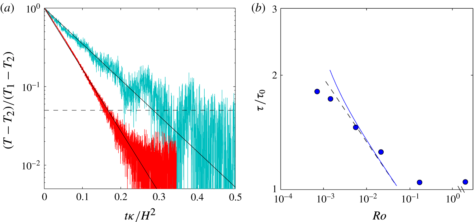
The temperature equilibration in rotating experiments took the same exponential form (4.1) as previously found for the non-rotating case (figure 2
a). Approximately 99 % of the overall temperature change is shown in figure 2(a), and the exponential describes more than 95 % of that adjustment. At larger times the difference between the time-dependent interior temperature
 $T$
and the final, time-averaged interior temperature
 $T_{2}$
was smaller than the interior temperature fluctuations. The fluctuations at a single measurement position in the interior in the equilibrium states involved a spectrum of frequencies (see § 8), with amplitudes approximately 1 %–3 % of the maximum temperature difference
 $\unicode[STIX]{x0394}T$
in the final state, and they were largest in the rotating cases owing to unsteady vortical plumes, geostrophic eddies and basin-scale gyres.
Thermal equilibration for
 $Ra_{F}\approx 6\times 10^{14}$
. (a) Time records of bulk temperature (at
 $x/L=0.92$
,
 $y/W=0.5$
and
 $z/H=0.5$
), where temperature relative to the final time-averaged interior
 $T-T_{2}$
is normalised by the total difference
 $T_{1}-T_{2}$
between final and initial states, and time is normalised by
 $H^{2}/\unicode[STIX]{x1D705}$
. Solid black lines are the exponential relation (4.1) fitted to the non-rotating (
 $f=0$
; red curve) and the most rapidly rotating (
 $f=1.6~\text{s}^{-1}$
,
 $Ro=7.1\times 10^{-4}$
; cyan curve) cases, giving time scales
 $\unicode[STIX]{x1D70F}_{0}=1.44\times 10^{4}~\text{s}$
and
 $\unicode[STIX]{x1D70F}=2.71\times 10^{4}~\text{s}$
, respectively. Broken line indicates the value corresponding to 95 % of the complete adjustment to the final temperature. (b) Rossby number dependence of measured equilibration time scales normalised by the non-rotating scaling (4.2) with
 $c_{2}=2.0$
(from fit of (2.10) to measured boundary layer results over the cooled region in equilibrium state, see figure 7). The single data point after the axis break shows the measured adjustment time scale in the non-rotating case. Broken line is the geostrophic boundary layer scaling (4.3) and solid blue line is the geostrophic boundary layer scaling with a correction for isopotential curvature (A 3 in appendix A), both with fitted prefactor
 $c_{10}=0.89$
.
Plan view image showing the positions at which dye tracer was released on the base, along with an example of the initial paths of the tracer while it was largely in the bottom boundary layer. The photograph is from Experiment 4 (table 1;
 $Ra_{F}=6.5\times 10^{14}$
,
 $f=0.4~\text{s}^{-1}$
,
 $Ro=5.6\times 10^{-3}$
). Base heating is on the left-hand side and cooling on the right-hand side. At positions 1 and 2 blue dye was released, at position 3 red dye was released, within 1 mm from the base. System is in the geostrophic boundary layer regime (as discussed in § 6). See figure 4 for side view.

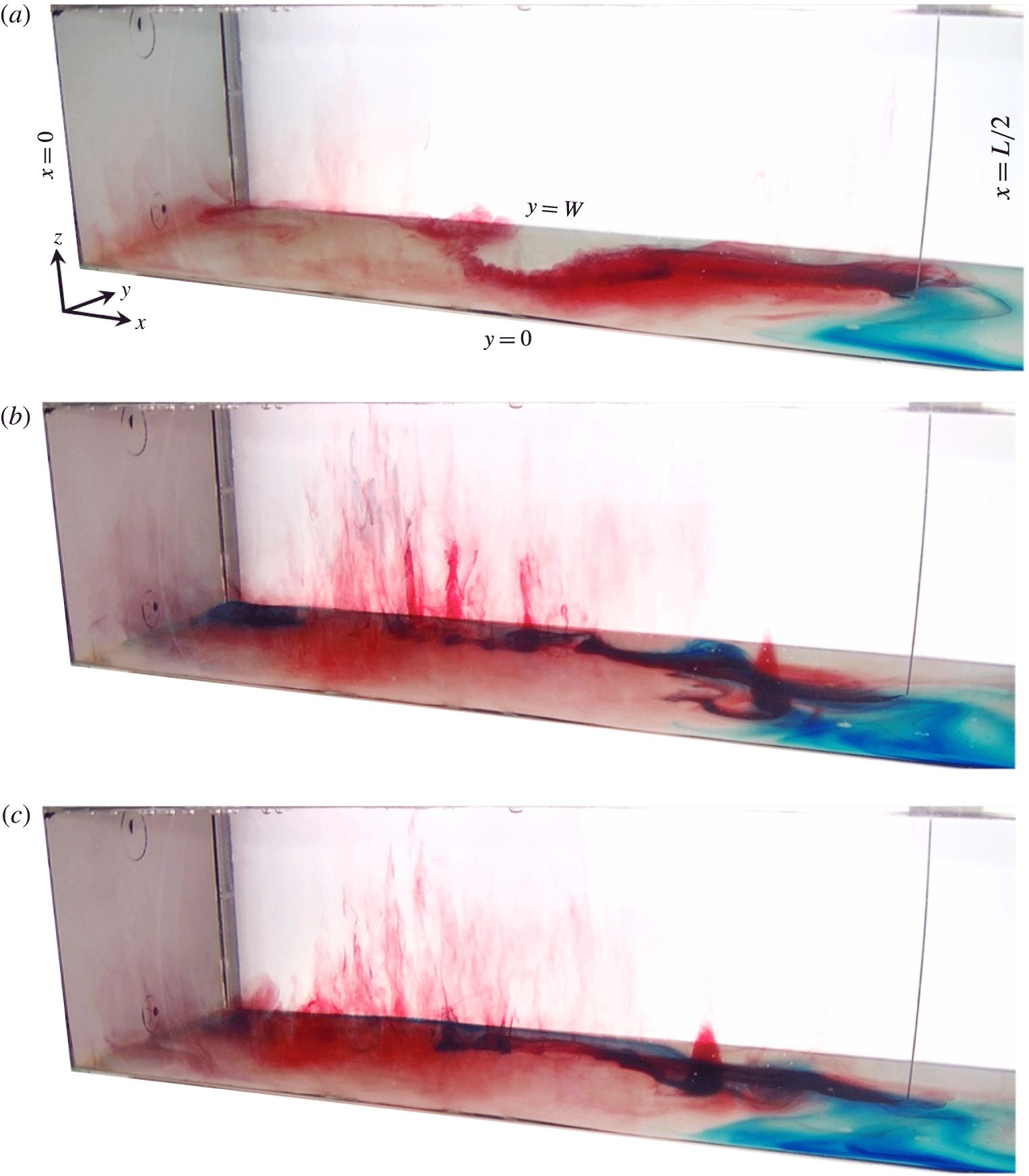
Side view images from Experiment 4 (as in figure 3) with dye tracer and showing only the heated half of the box (
 $Ra_{F}=6.5\times 10^{14}$
,
 $f=0.4~\text{s}^{-1}$
,
 $Ro=5.6\times 10^{-3}$
) at (a) 19 mins, (b) 23 mins and (c) 57 mins, respectively, after dye release began. System is in the geostrophic boundary layer regime (as discussed in § 6). See supplementary movie 1.

Side view images from Experiment 6 with dye tracer and showing only the heated half of the box (
 $Ra_{F}=6.8\times 10^{14}$
,
 $f=1.6~\text{s}^{-1}$
,
 $Ro=7.1\times 10^{-4}$
) at (a) 18 mins, (b) 22 mins and (c) 22 mins 40 s, respectively, after dye release began. System is in the inertial chimney regime (as discussed in § 6). See supplementary movie 2.
For strong rotation (
 $Ro<10^{-1}$
) the adjustment time scales were larger (figure 2
b). The Rossby number dependence was not as strong as that predicted by the geostrophic boundary layer scaling (4.3), but the difference can be attributed to the transitional behaviour of the Nusselt number (i.e. higher interior temperatures) with significant Ekman transport in the equilibrium states for
 $Ro>10^{-3}$
, and a change over to Nusselt numbers larger than predicted by the geostrophic boundary layer scaling (i.e. smaller interior temperatures) at
 $Ro<10^{-3}$
(see § 6). As an estimate of the equilibration time scales, we simply report that a best fit of the geostrophic boundary layer scaling (4.3) to the data in the range
 $10^{-3}<Ro<10^{-1}$
gives the prefactor
 $c_{10}\approx 0.9$
, and note that all of the measured time scales indicate
 $\unicode[STIX]{x1D70F}<0.1H^{2}/\unicode[STIX]{x1D705}$
.
5 Flow visualisation
An example of the flow patterns revealed by the tracer advection in the rotating cases (and which will be shown to be an example of the geostrophic boundary layer regime) is shown in figure 3. There are supplementary movies online available at https://doi.org/10.1017/jfm.2017.249 with a side view of the box for this experimental run,
 $Ra_{F}=6.5\times 10^{14}$
and
 $Ro=5.6\times 10^{-3}$
(Experiment 4; still photos shown in figure 4; movie 1), and at stronger rotation,
 $Ra_{F}=6.8\times 10^{14}$
and
 $Ro=7.1\times 10^{-4}$
(Experiment 6; stills in figure 5; movie 2). As shown in figure 3, the blue tracer released at position 1 (marked on the image), which was on the cooled base, remained close to the wall (
 $y/W=1$
), as it was carried towards the end wall (
 $x/L=1$
). It continued around the box against the end wall to the opposite ‘western’ side wall (
 $y/W=0$
) and then along the wall towards the heated region. (We use the terms ‘western’ or ‘eastern’ here for convenience, and they are based on the northward direction of the net boundary layer flow in a northern hemisphere ocean basin, with west on the left, despite there being no mechanism similar to the planetary
 $\unicode[STIX]{x1D6FD}$
-effect to provide east–west asymmetry in these experiments.) The dyed water released at position 2 near the ‘western’ side wall showed the same flow pattern, the tracer being carried directly along the side wall, with the wall on its left, to the heated region. Thus the flow in the cooled region of the boundary layer was a large-scale anticyclonic (clockwise) gyre. The boundary layer flow in this region was always laminar, and relatively slow compared to that over the heated region of the base.
Tracer released in the centre of the base at position 3 was carried toward the heated region. Both the red and blue streams were diverted to the right of their direction of motion and across to the side wall (
 $y/W=1$
) over the heated base. In particular, the streamlines of cold boundary layer water entering the heated region near the wall
 $y/W=0$
(with blue dye) crossed the box on average about half-way along the heated region (under the conditions of this experiment). The boundary layer was unstable, stream-parallel rolls appearing a short distance from the leading edge of the heated region of the base and then breaking up into three-dimensional turbulent convection within the boundary layer approximately 100 mm further along in the direction of flow. In the region
 $x/L<1/4$
the flow showed large variability. The mean flow tended to form a cyclonic (anticlockwise) gyre having approximately equal length and width, filling the width of the box. In this region the boundary layer continued to warm as it circulated, and the water then ascended into the interior in vertical convection that appeared to be dominated by cyclonic vortical plumes.
More detail of the three-dimensional flow pattern could be seen in simultaneous side (or oblique) views such as those shown in figure 4, which are from the same experiment as that in figure 3. The thin streams of tracer over the cooling region of the base are testament to the strong density gradient there. The roll instability and three-dimensional small-scale convection in the boundary layer stir and mix the tracer through a larger fraction of the boundary layer thickness. The stream of red dye reveals vertical convection at the end wall under the conditions in this experiment, particularly at the far corner (
 $x/L=0,y/W=1$
). However, strong vortical plumes formed elsewhere over the heated region and most commonly in the area where the stream of cold boundary layer water (with blue dye) crossed the box near
 $x/L\approx 1/4$
adjacent to the warming cyclonic gyre. The variability was such that at times the cold stream warmed sufficiently that the vortical plumes carried only the blue dye upward out of the boundary layer (figure 4
b) and at other times the stream carrying the red dye along near the far side wall was diverted into the middle of the heated region of the base and the vortices carried the red dye upward (figure 4
c). This fluctuation in the larger-scale circulation occurred every 20–30 min. There were generally one or two plumes at a time. Each vortical plume remained coherent for several minutes before breaking up. The vortical plumes could generally be seen all the way to the lid of the box. In the interior the tracer carried up by plumes became broadly dispersed and on average they (and the tracer) migrated toward the cooled end of the box. The tracer was stirred laterally until it eventually filled the whole of the interior. As a result of these relatively rapid motions, it was not possible to determine from the dye any further detail of larger-scale mean horizontal circulation in the interior.
At larger rotation rates some aspects of the flow pattern changed. The strongly stable boundary layer over the cooled half of the base again formed a large-scale anticyclonic gyre. As shown in figure 5, the current along the near (western) wall (
 $y/W=0$
) was diverted across the box towards the far wall at a position closer to the leading edge of the basal heating when compared to smaller rotation rates at around the same Rayleigh number. Over the heated area of the base the boundary layer was again unstable to small-scale convection. It tended to flow to the left near the far wall and there was again a tendency for a cyclonic gyre circulation filling the width of the box at the heated end. However, under the more rapid rotation there were many more vortical plumes and these occurred over a larger area. We will refer to this region of vortical plumes as a convection ‘chimney’, borrowing previous ocean modelling terminology for regions of open ocean deep convection. In this case less tracer made it all the way to the end wall (
 $x/L=0$
), and there was little evidence of tracer being carried upward by vertical convection adjacent to the end wall. Most of the tracer was instead carried upward in the vortical plumes in the chimney over the central region of the heated area. The vortical plumes extended through the full depth of the box, from the base to the lid.
The red dye also revealed the cone-like structure in the right-hand half (
 $x/L=0.4$
,
 $y/W=0.5$
) of figure 5(b,c). This cone was at the base of a vortical plume in the interior, but in this case the tracer did not flow further up through the interior, implying a persistent stable stratification within that vortical plume, above the boundary layer. The cone moved with a velocity that was decoupled from the underlying mean boundary layer flow, and migrated towards the cooled region of the base where it slowly dispersed.
While convection in the chimney region at small values of the convective Rossby number involves vortical plumes similar to flow structure seen in rotating convection above a uniformly heated plate or in rotating Rayleigh–Bénard convection between two horizontal boundaries (Chandrasekhar Reference Chandrasekhar1953; Boubnov Reference Boubnov1984; Boubnov & Golitsyn Reference Boubnov and Golitsyn1986, Reference Boubnov and Golitsyn1990; Julien et al. Reference Julien, Rubio, Grooms and Knobloch2012; Aurnou et al. Reference Aurnou, Calkins, Cheng, Julien, King, Nieves, Soderlund and Stellmach2015), it is important to recall that the two cases are crucially different. In the state of thermal equilibrium studied here, horizontal convection must involve a balance between the large-scale lateral flow and the vertical convection above the heated region that is crucial to the flow achieving zero net buoyancy flux through any level. This coupling of lateral and vertical transport leads to a stably stratified thermal boundary layer, as well as to a gravitationally stable mean stratification throughout the interior volume. Gravitationally unstable stratification is found only locally in the plumes and in a sublayer at the heated base (very much thinner than the main thermal boundary layer). In contrast, Rayleigh–Bénard convection achieves a balance of heat input through the base and heat withdrawn through the upper boundary, with thermal boundary layers and interior volume that are gravitationally unstable. Associated with these differences in buoyancy flux and stratification is a large difference in rates of viscous dissipation, as previously demonstrated for non-rotating horizontal and Rayleigh–Bénard convection at large Rayleigh numbers (Gayen et al. Reference Gayen, Griffiths, Hughes and Saenz2013a ; Gayen, Hughes & Griffiths Reference Gayen, Hughes and Griffiths2013b ; Hughes, Gayen & Griffiths Reference Hughes, Gayen and Griffiths2013) and which have been shown to be little affected by rotation until extreme rotation rates are reached (Vreugdenhil et al. Reference Vreugdenhil, Gayen and Griffiths2016).
6 Scaling comparison
Vertical profiles of temperature, shown for the region above the cooled end of the base in figure 6(a), reveal a strongly stratified region (the thermal boundary layer) at the base and a relatively weak stratification through the remainder of the depth. In the range
 $10^{-1}>Ro>10^{-3}$
the interior temperature is larger and the boundary layer is thicker for larger rotation rates. Noting that
 $T-T_{c}\approx \unicode[STIX]{x0394}T\sim Nu^{-1}$
for imposed heat flux, these changes are consistent with the geostrophic boundary layer regime (2.17). These trends are also consistent with the laboratory experiments of Park & Whitehead (Reference Park and Whitehead1999). The interior temperature remains in the range
 $T-T_{c}=(0.88{-}0.95)\unicode[STIX]{x0394}T$
. The buoyancy frequencies (figure 6
b) calculated from the temperature profiles reveal a near-base portion of the boundary layer in which rotation does not change the stratification, or slightly reduces it. In contrast, in the outer boundary layer the effects of rotation increase the buoyancy frequency. The stratification in the bulk of the fluid similarly increases with increasing rotation rate. Indeed the density gradient in the interior was almost an order of magnitude greater for weak rotation (
 $Ro=1.7\times 10^{-1}$
) than for the non-rotating case, and was a further order of magnitude greater at rapid rotation (
 $Ro\approx 10^{-3}$
). At
 $Ro<10^{-3}$
the behaviour is different: the boundary layer continued to thicken with increasing rotation rate, whereas the interior temperature trends are reversed, with the interior cooling slightly and becoming less stratified for more rapid rotation. Further details of the boundary layer behaviour, Nusselt number and mass transport are given below.
Profiles of (a) temperature and (b) squared buoyancy frequency
 $N$
with depth for
 $Ra_{F}\approx 6\times 10^{14}$
and different rotation rates. Shown are time-averaged profiles from the equilibrium state measured above the cooled region of the base (
 $x/L=0.92$
,
 $y/W=0.5$
). In (a) the profiles are linearly interpolated (broken lines) between
 $z/H=0.0075$
and the temperature
 $T_{c}$
measured in the cooled end of the base. Temperatures are relative to
 $T_{c}$
and are normalised by the overall difference
 $\unicode[STIX]{x0394}T_{0}=(T_{h}-T_{c})_{0}$
along the base in the non-rotating case;
 $N^{2}$
is normalised by the fixed value of
 $N_{0}^{2}=g\unicode[STIX]{x1D6FC}\unicode[STIX]{x0394}T_{0}/H$
based on the measured
 $\unicode[STIX]{x0394}T_{0}$
in the non-rotating case.
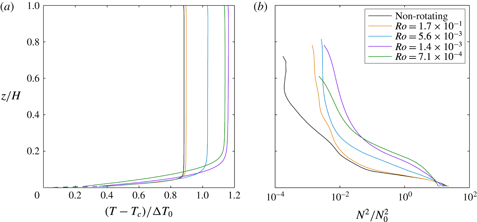
6.1 Boundary layer thickness
The boundary layer thickness is defined here as the height from the base containing 90 % of the top-to-bottom buoyancy difference. The thickness varies with location as a result of geostrophic horizontal flow, including the circulation gyres on the scale of the box and side wall boundary currents. It also varies with distance from the axis of rotation due to parabolic curvature of isopotential surfaces (appendix A). Over the cooled region the boundary layer is thinner for larger Rayleigh numbers and thicker for more rapid rotation (figure 7
a). Rotation begins to influence the boundary layer at
 $E<10^{-5}$
given the other experimental conditions. The effect of rotation is seen more clearly in figure 7(b), where all thickness measurements are normalised by the thickness given by the scaling law (2.10) for the non-rotating case. When comparing the measured thickness at this location near the ends of the box with theoretical predictions, a correction is added to the predicted thickness scaling in order to account for the parabolic curvature of isopotential surfaces (appendix A). In figure 7(b) the geostrophic boundary layer scaling (2.18) with the correction for isopotential curvature matches the measured boundary layer thicknesses in the range
 $Ro<10^{-1}$
. The data are consistent with past experimental results at smaller Rayleigh number (Park & Whitehead Reference Park and Whitehead1999). The transition to the geostrophic boundary layer regime starts at
 $Ro\approx 10^{-1}$
.
(a) Boundary layer thickness near the cooled end (at
 $x/L=0.92$
,
 $y/W=0.5$
) against Ekman number and (b) the boundary layer thickness normalised by the non-rotating scaling against Rossby number for three different
 $Ra_{F}$
. The three data points after the axis break show the measured boundary layer thicknesses in the non-rotating cases. In (a) the broken lines are the geostrophic boundary layer scaling (2.15) and the solid curves are that scaling with a correction for isopotential curvature (A 1 in appendix A), both with
 $c_{4}=1.96$
. The horizontal dotted line indicates the box height. In (b) the normalisation uses the non-rotating scaling (2.10) for
 $\unicode[STIX]{x1D6FF}_{0}$
fitted to the three non-rotating results, which give
 $c_{2}=2.0$
. The broken line is the normalised geostrophic boundary layer scaling (2.18) and the solid curves are that scaling with the isopotential curvature correction (A 2), all with prefactor
 $c_{6}=0.97$
. In (a) the non-rotating
 $Ra_{F}\approx 6\times 10^{14}$
(blue circle) case lies underneath the
 $Ra_{F}\approx 1\times 10^{14}$
(red triangle) case.
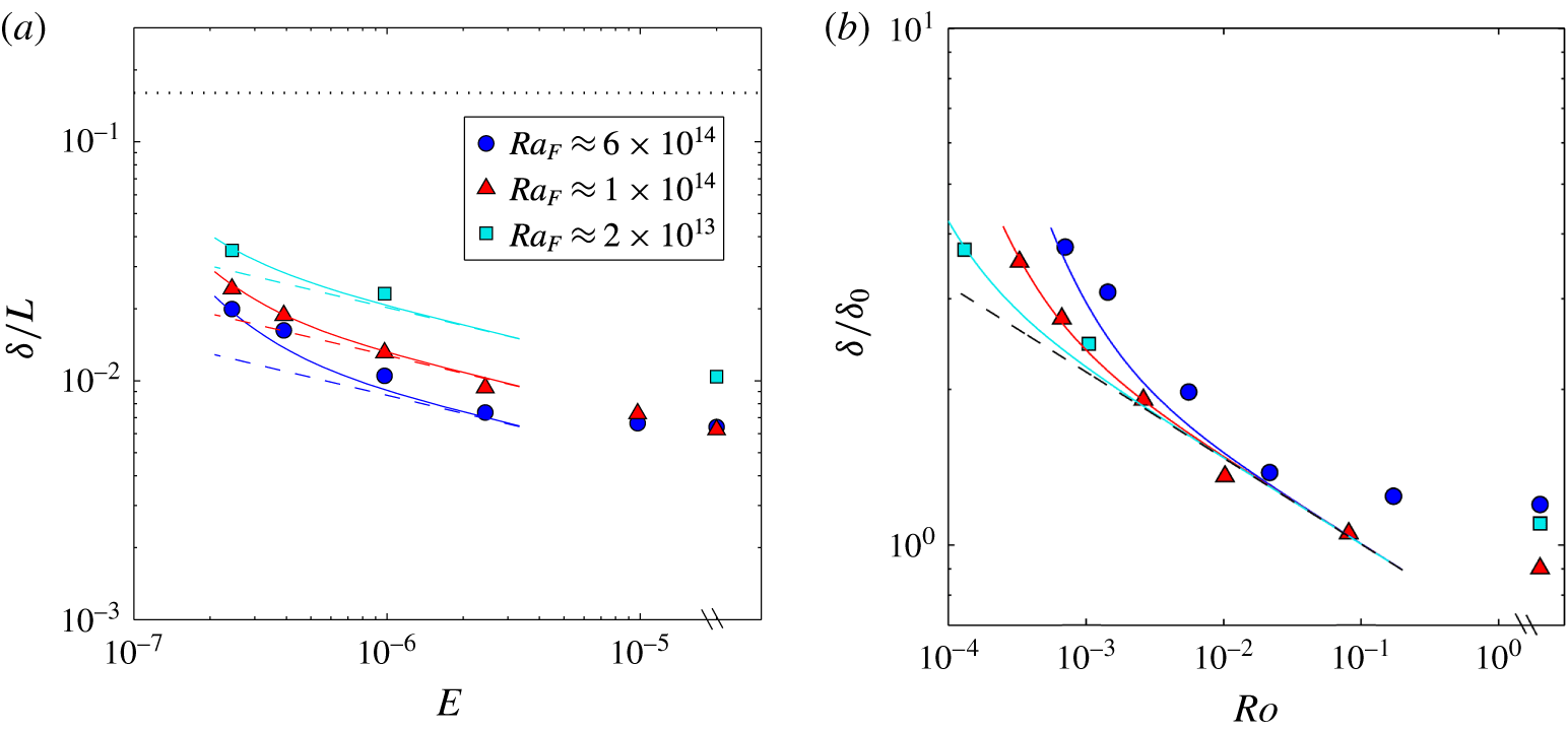
The boundary layer becomes more variable with increasing rotation rate. Figure 8 shows the normalised boundary layer thicknesses at three locations across the mid-section (
 $x/L=0.5$
) of the box. The boundary layer is asymmetric in the presence of rotation and the thickness trends depend on the cross-stream location. Near the ‘western’ wall (left-hand side when looking in the direction of net boundary layer flow;
 $y/W=0.027$
) the boundary layer thickness remains unchanged by rotation until
 $Ro<10^{-3}$
, and at stronger rotation it becomes thinner. At the centre point of the box (
 $y/W=0.5$
) the boundary layer is thicker for stronger rotation if
 $Ro>10^{-3}$
but becomes thinner at
 $Ro<10^{-3}$
. Near the ‘eastern’ wall (
 $y/W=0.973$
) the thickness monotonically increases for stronger rotation, in a manner consistent with the geostrophic boundary layer scaling (2.18). Thus the boundary layer thickness is again largely consistent with the geostrophic boundary layer scaling at
 $10^{-3}<Ro<10^{-1}$
, but there is more complex behaviour at
 $Ro<10^{-3}$
.
Boundary layer thickness on the mid-section of the domain (
 $x/L=0.5$
) at (a)
 $y/W=0.027$
, (b)
 $y/W=0.5$
and (c)
 $y/W=0.973$
. Boundary layer thickness is normalised by the non-rotating scaling (2.10) fitted to the non-rotating results (the points after the axis break), which give
 $c_{2}=1.7$
for all cases. The solid line is the geostrophic boundary layer scaling (2.18) with prefactors (b)
 $c_{6}=1.26$
and (c)
 $c_{6}=1.09$
. The averaged thickness across the width at
 $x/L=0.5$
is shown in figure 11(c).
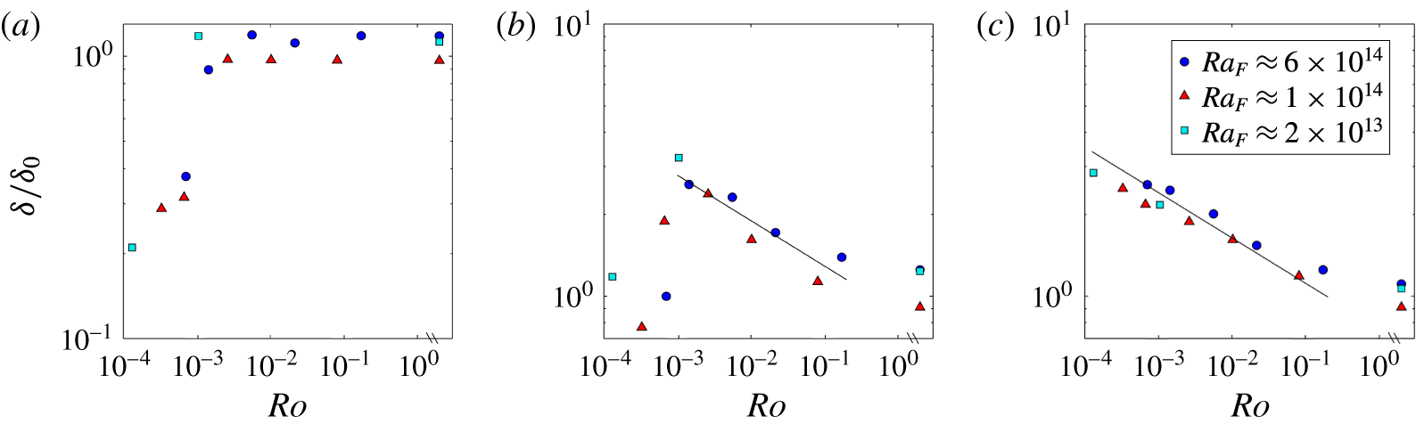
6.2 Nusselt number
In the case of imposed heat flux the (inverse) Nusselt number (2.2) serves as the dimensionless measure of temperature differences in the flow. The Nusselt number is measured as the time-averaged temperature difference
 $\unicode[STIX]{x0394}T$
between the heated (where
 $T_{h}$
was from the single functioning thermistor) and cooled (where
 $T_{c}$
was the mean of two thermistors) regions of the plate. The Nusselt number, shown normalised by non-rotating values for each Rayleigh number in figure 9, is smaller for smaller heat flux or more rapid rotation, and hence for smaller Rossby number. However, the dependence is weaker than predicted by the geostrophic boundary layer scaling (2.18). Across the full range of conditions achieved, the dimensionless temperature difference required to drive the imposed heat flux increased by only 20 %. A similar trend was found by Park & Whitehead (Reference Park and Whitehead1999), over a small range of Coriolis parameter, and it was argued that the simple geostrophic boundary layer scaling requires a correction to account for the volume and heat transport in the Ekman layer (which we extend to the present Rossby number expressions in appendix B). The Ekman transport correction is negligible at very small
 $Ro$
and becomes large when the Ekman layer approaches the thickness of the thermal boundary layer (at
 $Q\approx 1$
or
 $Ro\approx 10^{-1}$
) and there is no longer a significant geostrophic part of the boundary layer. Thus in figure 9 the Ekman corrected geostrophic boundary layer scaling (B 1) is shown up to
 $Ro\approx 5\times 10^{-2}$
beyond which its formulation is invalid. The correction provides an estimate of the expected flow in transitional conditions (the weak rotation regime of Hignett et al. (Reference Hignett, Ibbetson and Killworth1981)) between the non-rotating regime and the strong rotation (geostrophic) regime. The present results place the transitional regime at
 $10^{-2}<Ro<10^{-1}$
, although the magnitude of the Ekman correction to the scaling remains significant (compared with the data uncertainties) for
 $Ro<10^{-3}$
. A correction for thickening of the thermal boundary layer toward the end of the box (figure 7) resulting from the curvature of isopotential surfaces decreases the predicted Nusselt number (as
 $Nu\sim \unicode[STIX]{x1D6FF}^{-1}$
averaged over the area of the cooling boundary). The results show that the dynamics in the laboratory basin follows the geostrophic boundary layer scaling over only a small range of Rossby numbers, within
 $10^{-3}<Ro<10^{-2}$
.
Nusselt number as a function of Rossby number, where the Nusselt number is based on
 $\unicode[STIX]{x0394}T$
and normalised by the non-rotating scaling (2.10) fitted to the three non-rotating results (the points after the axis break), which gives
 $c_{3}=0.47$
. Both the broken curve and the dotted curve are the geostrophic boundary layer scaling (2.18) with different prefactors; the unbroken black curve is the geostrophic boundary layer scaling corrected for Ekman transport ((B 1); Park & Whitehead Reference Park and Whitehead1999); the coloured solid curves for three different
 $Ra_{F}$
are the stress-free geostrophic boundary layer scaling corrected for effects of curvature of isopotential surfaces (A 4). The prefactor
 $c_{7}=1.6$
is used for all rotating scaling, excepting the dotted curve geostrophic boundary layer scaling (2.18) which has
 $c_{7}=1.45$
. Error bars are dominated by the heat flux uncertainty, which is shown as the fraction (at most 4 %) of heat input lost from the box to the room and is estimated from calibrations of the heat loss (Stewart et al.
Reference Stewart, Hughes and Griffiths2011). Since the error is always a heat loss, the bars only extend downward. The vertical and horizontal axes are both logarithmic.
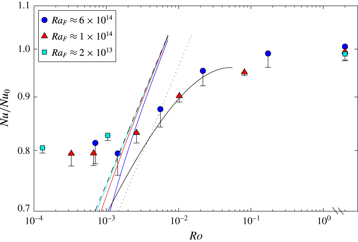
The Nusselt number results become largely independent of Rossby number at
 $Ro<10^{-3}$
, meaning that the temperature difference required to drive the imposed heat flux was approximately constant at larger rotation rates. For the largest heat flux the interior temperature was even observed to be smaller at the largest rotation rate (hence
 $Nu/Nu_{0}$
is larger) compared with the second largest
 $f$
, as is also seen from the profiles in figure 6. This strong deviation of the Nusselt number from the geostrophic boundary layer scaling is in the opposite direction from Ekman transport or isopotential curvature effects and inhibits the net transport of heat. These data are, on the other hand, consistent with the behaviour predicted for the inertial chimney regime (2.24), (2.25), specifically the absence of a dependence of Nusselt number on rotation rate. An estimate of the prefactor in (2.24) from the data is
 $c_{9}\approx 2\times 10^{-2}$
. The deviation from the geostrophic boundary layer scaling at
 $Ro\approx 10^{-3}$
is consistent with the sudden change in behaviour of the boundary layer thickness (figure 8), which decreased rapidly with further increases in
 $Ro$
across at least the ‘western’ half of the box width at the mid-section, leaving only the ‘eastern’ portion of the boundary layer continuing to increase in the manner predicted by the geostrophic boundary layer scaling.
6.3 Thermal wind and boundary layer transport
For the rotating cases with
 $Ro<10^{-1}$
a geostrophic balance is assumed to dominate much of the flow field, especially in regions with a strong vertical buoyancy gradient that inhibits vertical motion and sustains quasi-horizontal motion. Geostrophy may break down where convection drives strong vertical motion, in strong vortices having large relative vorticity, and at the small scales of turbulence, for which a local Rossby number is large. Thus the larger scales of the flow in the thermal boundary layer through the mid-section of the box (
 $x/L=0.5$
) are expected to be closely approximated by geostrophic balance and we use the thermal wind equation to find the geostrophic velocities and the net boundary layer transport through this section. This transport serves as a measure of net overturning transport given that all of the boundary heat input to the box is on one side of this section, and all of the heat withdrawal is on the other side.
There were five thermistors at
 $x/L=0.5$
spanning the cross-stream
 $y$
-direction. The thermal wind equation (2.12) between two adjacent temperature profiles a distance
 $\unicode[STIX]{x0394}y$
apart gives
 $$\begin{eqnarray}\frac{\unicode[STIX]{x2202}u}{\unicode[STIX]{x2202}z}=-\frac{\unicode[STIX]{x1D6FC}g}{f}\frac{\unicode[STIX]{x0394}T}{\unicode[STIX]{x0394}y}\end{eqnarray}$$
and profiles of the velocity component
 $u$
in the
 $x$
-direction were calculated from
 $$\begin{eqnarray}u(z)-u(z_{0})=(-\unicode[STIX]{x1D6FC}g/f)\int _{z_{0}}^{z}(\unicode[STIX]{x0394}T/\unicode[STIX]{x0394}y)\,\text{d}z,\end{eqnarray}$$
where
 $z_{0}$
is a reference level. A suitable reference level is one for which we have the best approximation of the velocity
 $u(z_{0})$
. The no-slip condition at the base was not useful because temperature profiles stopped at a distance
 $0.01H$
(2 mm) from the base, which was greater than the Ekman layer thickness (
 $\unicode[STIX]{x1D6FF}_{E}<0.01H$
for
 $Ro<10^{-1}$
). Another option could be to assume a velocity reversal at the top edge of the thermal boundary layer, which may apply on average, but a reversal is not required at each location in the presence of horizontal recirculation and the resulting thermal wind velocities were not consistent with velocity fields obtained from particle tracking velocimetry (see § 7.1). Hence the PTV measurements of horizontal velocities were used to reference the thermal wind profiles, choosing the PTV velocity field closest to the base (in the plane
 $z/H=0.15$
; see § 7.1), and to obtain the best estimate of the boundary layer transport. The calculated geostrophic velocities at
 $x/L=0.5$
, shown in figure 10 for the largest Rayleigh number and three rotation rates, thus include a reference velocity
 $u(z_{0}=0.15H)$
. The time-averaged temperature profiles were used. The three-dimensional results are complex. For example, the time-averaged geostrophic velocities close to the base near the ‘eastern’ side wall (
 $y/W=0.903$
) change from negative (toward to heated end) for weak rotation (figure 10
a), to positive for strong rotation (figure 10
b), and then back to negative for extreme rotation (figure 10
a). The velocities near the ‘eastern’ and ‘western’ walls tend to be of opposite sign through most of the depth of the box, but on average across the transect the boundary layer velocities are negative and the interior velocities are positive. There is generally no indication of a decrease in velocity towards zero at the base, consistent with the Ekman layer lying entirely within the region for which there are no data.
Vertical profiles of horizontal geostrophic velocity
 $u$
through the mid-section of the domain (
 $x/L=0.5$
) assuming thermal wind balance for
 $Ra_{F}\approx 6\times 10^{14}$
and three different rotation rates: (a)
 $f=0.04~\text{s}^{-1}$
,
 $Ro=1.7\times 10^{-1}$
, (b)
 $f=0.4~\text{s}^{-1}$
,
 $Ro=5.6\times 10^{-3}$
and (c)
 $f=1.6~\text{s}^{-1}$
,
 $Ro=7.1\times 10^{-4}$
. Locations in the key are half-way between the thermistor profiles. In (c) only four thermistors worked, giving only three velocity profiles. Positive
 $u$
indicates movement from the heated end to the cooled end. Uncertainty bars are propagated from measurement errors
 $\unicode[STIX]{x1D70E}_{\unicode[STIX]{x0394}T}=0.02\,^{\circ }\text{C}$
,
 $\unicode[STIX]{x1D70E}_{\unicode[STIX]{x0394}y}=0.005$
m and
 $\unicode[STIX]{x1D70E}_{z}=0.001$
m. It is uncertain whether thermal wind approximates the horizontal velocity field in the interior above the cooled boundary, as vertical and horizontal velocities may be comparable there; nonetheless the computed profiles are shown through the full depth.
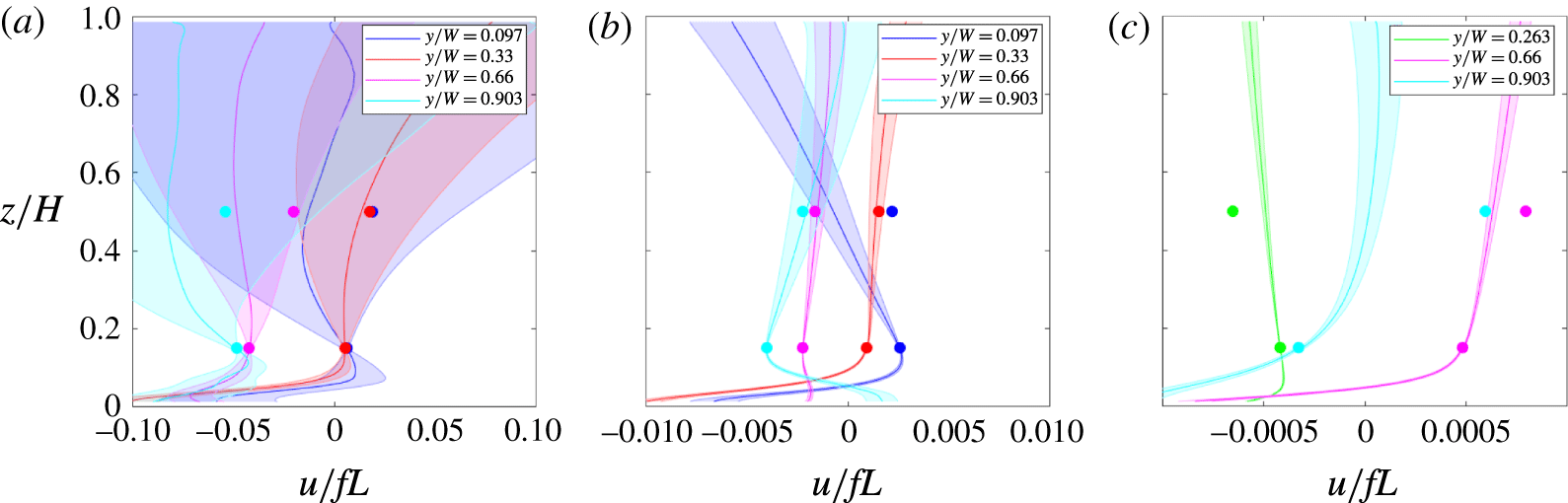
The geostrophic volume transport through each segment,
 $\unicode[STIX]{x1D6F9}_{i}$
, was found by integrating the thermal wind velocity over the (local) boundary layer depth and multiplying by the separation distance
 $\unicode[STIX]{x0394}y_{i}$
between each thermistor pair,
 $$\begin{eqnarray}\unicode[STIX]{x1D6F9}_{i}=\unicode[STIX]{x0394}y_{i}\int _{0}^{\unicode[STIX]{x1D6FF}_{i}}u_{i}(z)\,\text{d}z,\end{eqnarray}$$
where
 $i=1,n$
is the segment number and
 $\unicode[STIX]{x1D6FF}_{i}$
is the average boundary layer thickness in each segment. The net boundary layer transport through
 $x/L=0.5$
is the sum of the segment transports
 $\unicode[STIX]{x1D6F9}=\sum _{i=1,n}\unicode[STIX]{x1D6F9}_{i}$
. The thermistors closest to the side walls were at
 $y=0.0027W$
and
 $y=(1{-}0.0027)W$
(ie. 0.8 mm from the walls) and the transport in this region was not included. However, this neglects only a very small fraction of the total width and much of this is expected to be within a viscous side wall boundary flow with zero velocity at the walls.
The net transport can be written as
 $\unicode[STIX]{x1D6F9}=U_{av}\unicode[STIX]{x1D6FF}_{av}W$
, where the average boundary layer thickness
 $\unicode[STIX]{x1D6FF}_{av}$
across the box width is given by
 $$\begin{eqnarray}\unicode[STIX]{x1D6FF}_{av}=\frac{\displaystyle \mathop{\sum }_{i=1,n}(\unicode[STIX]{x0394}y_{i}\unicode[STIX]{x1D6FF}_{i})}{\displaystyle \mathop{\sum }_{i=1,n}\unicode[STIX]{x0394}y_{i}}.\end{eqnarray}$$
The transport in this problem is expressed in terms of the volume flux in preference over a volume flux per unit width of the box (as commonly used for the non-rotating horizontal convection problem) in view of both the three-dimensionality of the circulation and a possible dependence on the aspect ratio
 $W/L$
(which is not investigated in the experiments). The average velocity
 $U_{av}$
across the section is
 $U_{av}=\unicode[STIX]{x1D6F9}/\unicode[STIX]{x1D6FF}_{av}W$
, after taking
 $W\approx \sum _{i=1,n}\unicode[STIX]{x0394}y_{i}$
.
(a) The net volume transport (6.3) and (b) average geostrophic velocity in the
 $x$
-direction calculated from the thermal wind equation for the mid-section of the box for
 $Ra_{F}\approx 6\times 10^{14}$
, and (c) average boundary layer thickness (6.4) across the box at the mid-section (
 $x/L=0.5$
) for three Rayleigh numbers. The non-rotating transport used to normalise
 $\unicode[STIX]{x1D6F9}$
in (a) is given by (2.11) with numerical coefficient set to one given that the actual coefficient has not been evaluated. The velocity in (b) is normalised by the non-rotating scaling (2.10), with
 $c_{1}=0.29$
taken from past results (Mullarney et al.
Reference Mullarney, Griffiths and Hughes2004), as the thermal wind balance cannot be used for the non-rotating case. The boundary layer thickness in (c) is normalised by the non-rotating scaling (2.10) fitted to the three non-rotating experiments (the data points after the axis break), which give
 $c_{2}=1.7$
. The solid lines are the geostrophic boundary layer scaling ((2.19) and (2.18)) with (a)
 $c_{8}=0.44$
, (b)
 $c_{5}=0.80$
and (c)
 $c_{6}=1.09$
.
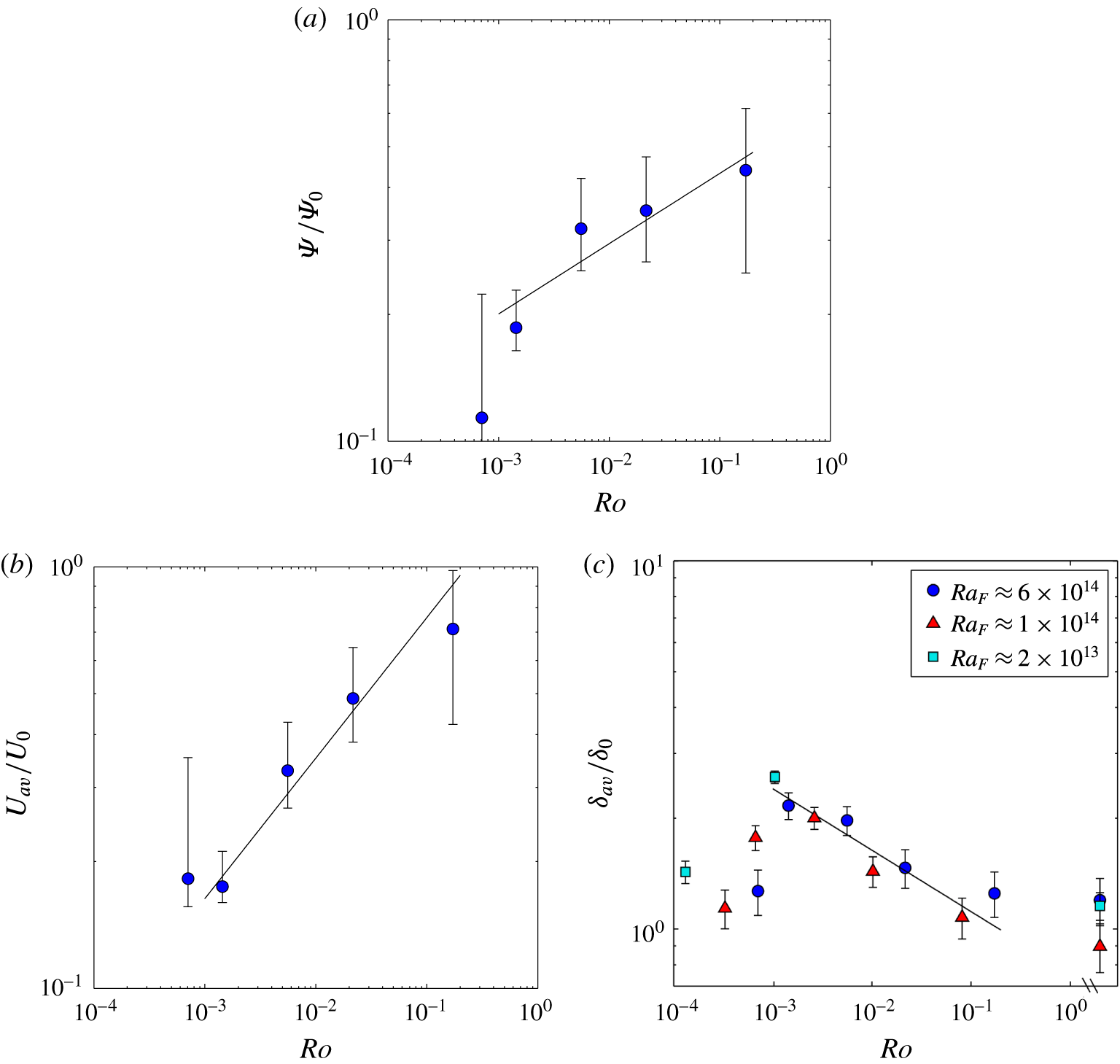
The calculated thermal wind transport and average velocities in the boundary layer, and the average boundary layer thickness at the mid-section of the domain are shown in figure 11, where the uncertainties include propagation of the uncertainties from the thermal wind profiles (coloured error bounds on figure 10) and allowances for the missing regions at the base and at the side walls. The transports include a correction using a simple linear interpolation of the velocity profiles to the base from its value at
 $z/H=0.01$
to zero at the boundary. The uncertainty estimate includes the difference in transport between this assumption and an alternative simple linear extrapolation of the velocity to a maximum at the edge of the Ekman layer (at
 $\unicode[STIX]{x1D6FF}_{E}=LE^{1/2}$
) and a linear decrease through the Ekman layer to zero velocity at the base. In most cases these extrapolations add to the net transport and therefore the uncertainty is asymmetric, the upper error bars in figure 11(a,b) being larger than the lower bars. The result at the smallest Rossby number has a larger uncertainty because this case had the thinnest Ekman layer and the temperature profiles do not extend as close to the expected height of the maximum velocity. All of the results are reasonably described by the geostrophic boundary layer scaling in the range
 $10^{-3}<Ro<10^{-1}$
. As foreseen from figure 11, the average boundary layer thickness at this mid-section deviates strongly from the scaling at
 $Ro<10^{-3}$
. However, the data for geostrophic transport and velocity were obtained only for a sequence of runs with the largest heat flux and are not sufficient to determine the behaviour of the average boundary layer velocity and transport at very small
 $Ro$
.
7 Interior velocity fields and overturning transport
7.1 Interior horizontal velocities
The PTV velocity fields obtained at 1 s intervals during the thermally equilibrated state indicated large-amplitude, low frequency fluctuations consistent with those inferred qualitatively from the dye tracer observations. Time-averaged velocity fields were obtained by averaging the instantaneous fields over periods of 20, 60 and 180 min after tracer particles were introduced and the results were approximately independent of the averaging period. As an additional test of whether the length of the averaging period was sufficient, one experiment (with
 $Ra_{F}=6.5\times 10^{14}$
and
 $Ro=5.6\times 10^{-3}$
) was repeated with a new fill of the tank and the two time-averaged velocity fields (from 3 h periods) taken at mid-depth were compared. To quantify the standard deviation between the two time-averaged velocity fields at mid-depth, we calculate the spatial average of the difference between the two velocity fields
 $\overline{u_{1}}(x,y)$
and
 $\overline{u_{2}}(x,y)$
as a fraction of the maximum speed in the
 $u_{2}$
field,
 $$\begin{eqnarray}\unicode[STIX]{x1D70E}_{m}=\frac{\displaystyle \mathop{\sum }_{i,j}|\overline{u_{1i,j}}-\overline{u_{2i,j}}|}{\text{max}|\overline{u_{2i,j}}|},\end{eqnarray}$$
where
 $i,j$
are the PTV windows in the field. The data give
 $\unicode[STIX]{x1D70E}_{m}=0.1$
, meaning that the two fields match to within 10 %. Thus we confidently use averages over 3 h (and 10800 frames) as faithful representations of the time-averaged horizontal flow.
For ‘weak rotation’ (
 $Ro=1.7\times 10^{-1}$
) a weak and basin-scale cyclonic gyre (having circulation in the same sense of the anticlockwise background rotation) occupied much of the domain, as shown in figure 12(a) (where the
 $u$
component at mid-depth is plotted along with contours of the two-dimensional horizontal streamfunction derived from the horizontal velocity field). At mid-depth the mean velocities on the ‘western’ side of the basin (
 $y/W<0.5$
) in this gyre were largely in the opposite direction to those in the underlying thermal boundary layer (where they are largely negative, figure 10
a), whereas on the ‘eastern’ side of the gyre the velocities were in the same direction as the boundary layer. However, when averaged across the box width at the mid-section of the box, the net flow was towards the heated end (in the same direction as the boundary layer transport). This became a more uniform motion toward the end wall in the region
 $x/L<0.2$
. A nearly uniform velocity
 $u$
tended to be maintained up to very close to the end wall, consistent with a significant vertical convection in a narrow region against the end wall. There was a second but much smaller region of cyclonic circulation above the ‘western’ corner of the heated region. The magnitude of the velocities at this Rossby number was everywhere less than
 $0.1fL$
, and not much smaller than the calculated geostrophic boundary layer speeds (figure 10
a). These observations are largely consistent with the (substantially less accurate) thermal wind calculations for the interior flow in figure 10(a). They are also similar to the circulation at mid-depth in the non-rotating experiments and in corresponding direct numerical simulations of the non-rotating case (Gayen et al.
Reference Gayen, Griffiths and Hughes2014). At this moderately large value of the Rossby number, the internal radius of deformation characterising the boundary layer flow,
 $\unicode[STIX]{x1D706}\approx (g\unicode[STIX]{x1D6FC}\unicode[STIX]{x0394}T\unicode[STIX]{x1D6FF})^{1/2}/f$
, or the inertial radius
 $\unicode[STIX]{x1D706}=U/f$
, is of the same order as the domain width (
 $\unicode[STIX]{x1D706}/W=RoL/W\approx 0.7$
). Hence this natural length scale is not available to determine the size of geostrophically balanced flow structures.
Velocity component
 $u$
in the
 $x$
-direction measured by PTV at mid-depth (
 $z/H=0.5$
) and contours of calculated streamfunction for
 $Ra_{F}=6.2\times 10^{14}$
and
 $Ro=1.7\times 10^{-1}$
(
 $f=0.04~\text{s}^{-1}$
): (a) time averaged (
 $\overline{u}$
) over 3 h and (b) an instantaneous field. The velocities are normalised by
 $fL$
(scale shown by colour bar); positive velocities (red) indicate flow to the right toward the cooled region. The streamfunction contours have equal spacing
 $\unicode[STIX]{x0394}\unicode[STIX]{x1D713}=4\times 10^{-5}~\text{m}^{3}~\text{s}^{-1}$
per unit depth: white contours indicate cyclonic (anticlockwise) circulation and grey is the zero contour.
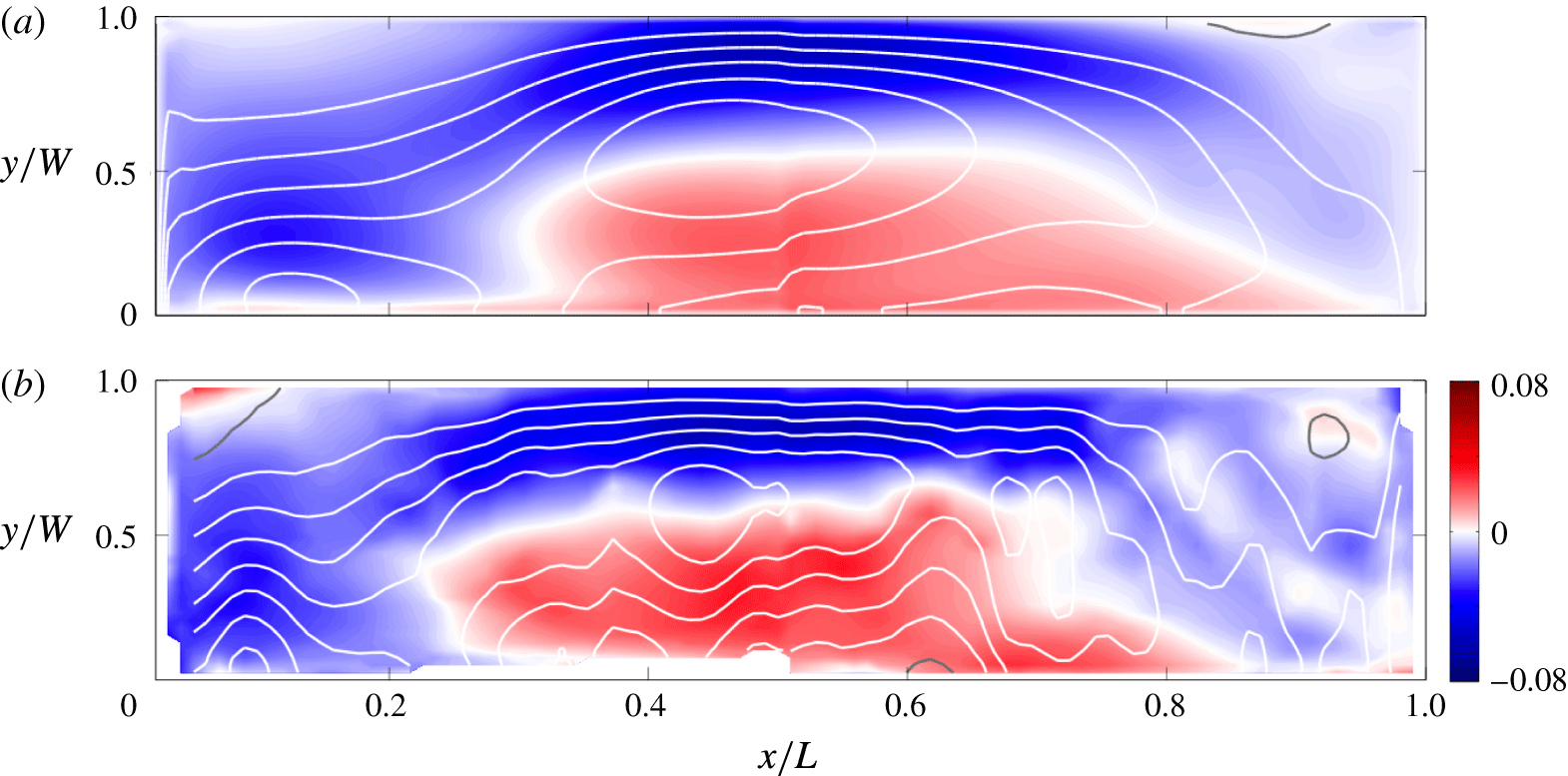
In contrast to the flow at mid-depth, the time average near the top of the domain (
 $z/H=$
0.85) shows a net flow through the mid-section directed towards the cooled end. This is similar to the return flow that closes the overturning circulation through the upper half of the depth in the non-rotating case. Adapting the measure defined in (7.1) to compare the time-averaged velocity fields at different depths we set
 $\overline{u_{1}}=\overline{u}(z/H=0.85)$
and
 $\overline{u_{2}}=\overline{u}(z/H=0.5)$
and replace
 $\unicode[STIX]{x1D70E}_{m}$
by
 $\unicode[STIX]{x1D70E}_{z}$
. We find
 $\unicode[STIX]{x1D70E}_{z}=0.7$
for
 $Ro=1.7\times 10^{-1}$
. Hence the velocities in the upper and mid-depth planes show that the flow varied substantially with height, although less so than that in the non-rotating case (in which we find
 $\unicode[STIX]{x1D70E}_{z}=1.5$
). The variability in the velocity field under these conditions is a significant fraction of the time average, but the general characteristics of the circulation described above reflect the instantaneous flow fields at nearly all times, as in the instantaneous field shown in figure 12(b). In particular there was no evidence of vortical plumes extending through the height of the box.
At a small value of the Rossby number (
 $Ro=5.6\times 10^{-3}$
), for which the boundary layer data in § 6 place the flow in the geostrophic boundary layer regime, the interior circulation was more substantially influenced by rotation: there were five basin-wide gyres along the length of the domain (figure 13
a). The time-averaged flow field, shown here for the PTV plane at mid-depth, in this ‘strong rotation’ case was much the same at all three PTV levels (
 $\unicode[STIX]{x1D70E}_{z}=0.13$
). The mean velocity fields were also mostly consistent with the time-averaged velocities calculated from thermal wind balance in the interior (figure 10
b) (although there were several discrepancies that may relate to uncertainties in the thermal wind calculation with very small horizontal temperature differences). Above the cooled region of the base there was a very weak anticyclonic gyre (indicated here only by the grey
 $\unicode[STIX]{x1D6F9}=0$
contour) that was largely overshadowed by two stronger cyclonic gyres. Above the heated region of the base there was a weak cyclonic region at the end of the box and a strong anticyclonic gyre, the latter having circulation comparable to the adjacent cyclonic gyre above the cooled base. Thus the mean horizontal circulation was concentrated in the central half of the basin, nearest the imposed gradient of thermal boundary conditions.
Velocity component
 $u$
from PTV at mid-depth and horizontal streamfunction contours for
 $Ra_{F}=6.5\times 10^{14}$
and
 $Ro=5.6\times 10^{-3}$
(
 $f=0.4~\text{s}^{-1}$
): (a) time-averaged over 3 h and (b–d) instantaneous fields (time interval from (b) to (c) is 3.7 min; (c) to (d) is
 $16.1$
min). Velocities are normalised by
 $fL$
; note that velocity colour scale is an order of magnitude smaller than in figure 12. Streamfunction contour spacing is
 $\unicode[STIX]{x0394}\unicode[STIX]{x1D713}=4\times 10^{-5}~\text{m}^{3}~\text{s}^{-1}$
per unit depth: white contours indicate cyclonic (anticlockwise) circulation, grey is the zero contour and black is anticyclonic circulation.
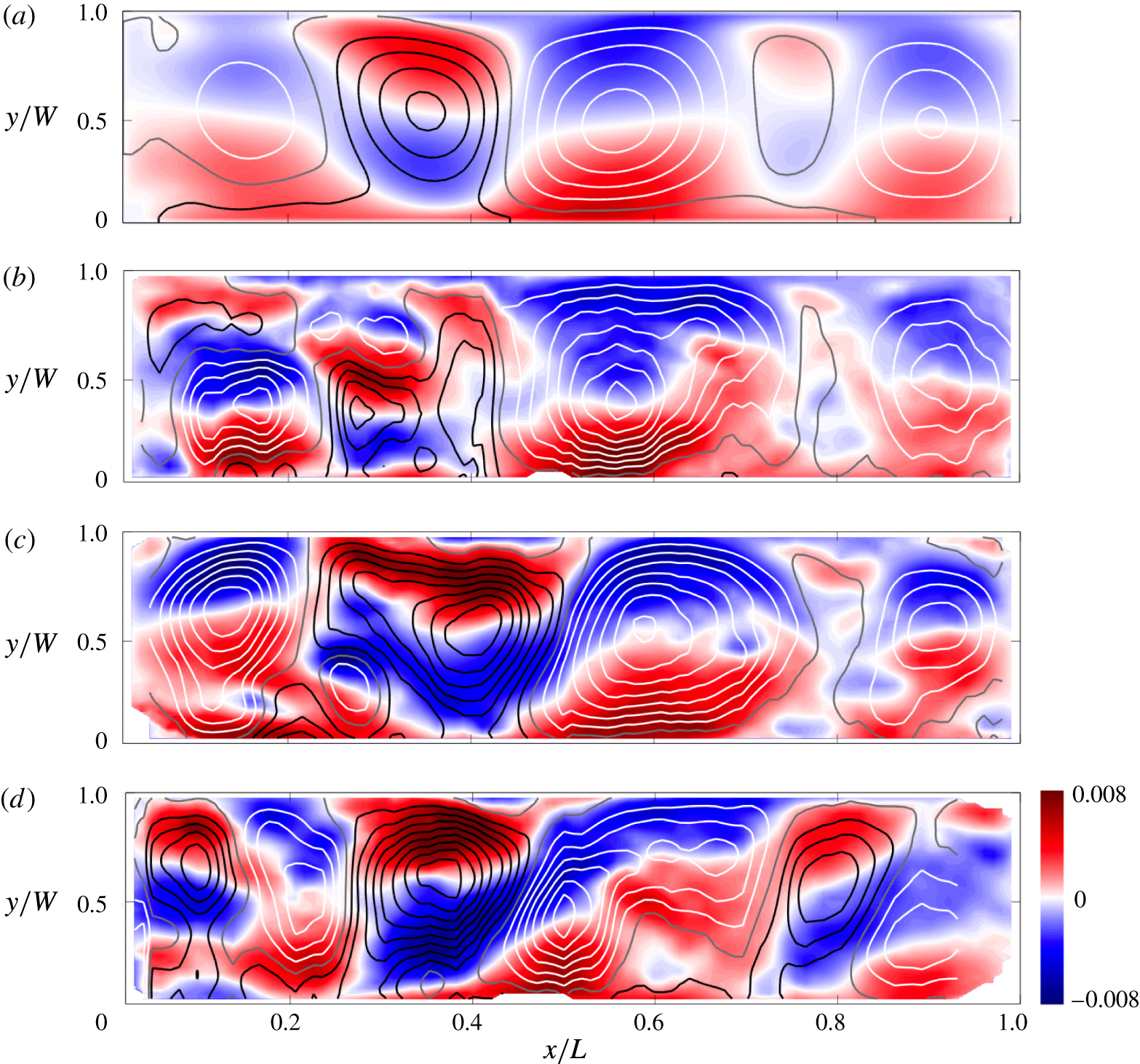
Instantaneous interior velocity fields at this small Rossby number (figure 13
b–d) show that the flow above the heated base experienced larger fluctuations compared to the ‘weak rotation’ case of figure 12. The strong anticyclonic gyre varied in shape and maximum transport, but was always present. The weak cyclonic gyre near the heated end of the basin was more variable, shifting its location and often splitting into two (cyclonic and anticyclonic) parts. Vertical convection (as seen with tracer advection in figure 4 and with the advection of fluorescein dye tracer in other runs with the PTV sheet illumination) can be linked to many of the smaller structures, which were also relatively short lived. In this experiment the Rossby radius of deformation was much smaller than the domain width (
 $\unicode[STIX]{x1D706}/W\approx 0.02$
) and could influence the size of flow structures, whether they were eddies formed by baroclinic instability or vortical plumes generated by vertical convection events. Above the cooled base the flow was less variable, although there was some fluctuations of the gyre structures.
At very strong rotation (
 $Ro=7.1\times 10^{-4}$
) the time-averaged velocity fields from PTV (shown for mid-depth in figure 14
a) show only two dominant gyres. The flow was again approximately independent of depth (
 $\unicode[STIX]{x1D70E}_{z}=0.07$
) and mostly consistent with the interior thermal wind results of figure 10(c). Circulation above the cooled half of the base was again predominantly cyclonic, but in this case formed a single gyre having larger lateral extent and smaller transport. The largest time-averaged interior velocities were associated with a large, strong anticyclonic gyre centred at
 $x/L\approx 0.4$
above the heated base but extending across the mid-section of the box. This anticyclonic gyre is therefore expected to provide an important contribution to the measured change in Nusselt number trend, as this mean flow will tend to transport heat more directly than the time-averaged flow pattern in figure 13. The mean flow was relatively weak near the end of the box above the heated base, consistent with the hypothesis that chimney convection above a large area of the heated base shifts the site of vertical heat transport away from an end wall plume and into an ‘open ocean’ chimney, despite the uniform heat flux boundary condition.
Velocity component
 $u$
from PTV at mid-depth and horizontal streamfunction contours for
 $Ra_{F}=6.8\times 10^{14}$
and
 $Ro=7.1\times 10^{-4}$
(
 $f=1.6~\text{s}^{-1}$
): (a) time-averaged velocity over 3 h and (b–d) instantaneous fields (time interval from (b) to (c) is 5.2 min; (c) to (d) is 9.3 min). Velocities are normalised by
 $fL$
; note the velocity colour scale is
 $1/4$
of that used in figure 13; streamfunction contour spacing is
 $\unicode[STIX]{x0394}\unicode[STIX]{x1D713}=4\times 10^{-5}~\text{m}^{3}~\text{s}^{-1}$
per unit depth.
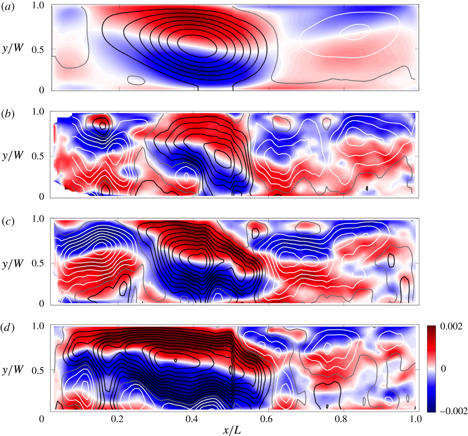
Instantaneous PTV velocity fields illustrated in figure 14(b–d) show that the strong anticyclonic gyre at such rapid rotation was present at all times, although it fluctuated very substantially in position, size and maximum transport (the transport varying in time by almost 50 %). Associated with these fluctuations were large changes in a transient, even more variable, cyclonic gyre close to the end wall. The fluctuations were of relatively high frequency, with time scales of a few minutes or 40–60 inertial periods. Smaller structures in the velocity field, such as the two or three small cyclonic eddies and two small anticyclonic eddies in figure 14(b), are consistent with a snap shot of vortical plumes penetrating through the depth of the box and the very small deformation radius (
 $\unicode[STIX]{x1D706}/W\sim 2\times 10^{-3}$
). The greater variability and smaller eddy scales at smaller values of the Rossby number are expected to contribute to lateral heat transfer in the chimney regime.
7.2 Overturning transport from PTV
An overturning transport was defined in § 6.3 as the net volume transport through the mid-section
 $x/L=0.5$
in the boundary layer and was estimated from temperature profiles assuming thermal wind balance. An independent estimate of the overturning is obtained from the interior velocity measurements, specifically from the horizontal divergence of velocity on any of the three PTV measurement planes. From the continuity equation (2.4) the vertical velocity
 $w$
and horizontal divergence satisfy
 $$\begin{eqnarray}\frac{\unicode[STIX]{x2202}w}{\unicode[STIX]{x2202}z}=-\unicode[STIX]{x1D735}_{h}\boldsymbol{\cdot }(u,v)\end{eqnarray}$$
and invoking the Taylor–Proudman theorem in the interior for strong rotation, giving (
 $u$
,
 $v$
) independent of depth, equation (7.2) is integrated to find the velocity
 $$\begin{eqnarray}w(z)-w(z_{0})=-(z-z_{0})\unicode[STIX]{x1D735}_{h}\boldsymbol{\cdot }(u,v),\end{eqnarray}$$
where
 $z_{0}$
is a reference height. At the edge of the Ekman layer on the upper boundary,
 $z_{E}=H-\unicode[STIX]{x1D6FF}_{E}=H-\sqrt{2\unicode[STIX]{x1D708}/f}$
and
 $w(z_{E})$
is the Ekman pumping velocity
 $$\begin{eqnarray}w(z_{E})=\left(\frac{\unicode[STIX]{x1D708}}{2f}\right)^{1/2}\unicode[STIX]{x1D735}_{h}\times (u,v).\end{eqnarray}$$
Hence we take
 $z_{0}=z_{E}$
at the upper boundary (which avoids the stratified bottom boundary layer) and (7.3) becomes
 $$\begin{eqnarray}w(z)=(H-\unicode[STIX]{x1D6FF}_{E}-z)\unicode[STIX]{x1D735}_{h}\boldsymbol{\cdot }(u,v)+{\textstyle \frac{1}{2}}\unicode[STIX]{x1D6FF}_{E}\unicode[STIX]{x1D735}_{h}\times (u,v).\end{eqnarray}$$
Overturning volume transport calculated from the horizontal divergence of the horizontal velocity fields from PTV at three vertical levels, normalised by the non-rotating scaling (2.11) with prefactor of one. The line shows the geostrophic boundary layer scaling (2.19) with prefactor
 $c_{8}=0.44$
and is the same line as in figure 11(a).
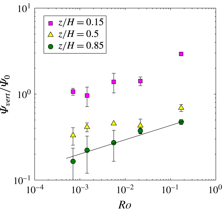
The vertical velocity was computed using (7.5) and the time-averaged horizontal velocity field on each of the three PTV measurement planes (
 $z/H=0.15$
, 0.5 and 0.85) for each experiment at the largest heat flux (
 $Ra_{F}\approx 6\times 10^{14}$
). The positive values of
 $w$
were integrated over the area of the plane to give a total upward transport
 $\unicode[STIX]{x1D6F9}_{pos}=\int _{0}^{W}\!\!\int _{0}^{L}w_{pos}(z)\,\text{d}x\,\text{d}y$
and separately the negative values of
 $w$
were integrated to give a total downward transport
 $\unicode[STIX]{x1D6F9}_{neg}=\int _{0}^{W}\!\!\!\int _{0}^{L}w_{neg}(z)\,\text{d}x\,\text{d}y$
. On figure 15 are plotted the average of the two
 $\unicode[STIX]{x1D6F9}_{vert}$
, and any difference between them is shown as an estimate of the uncertainty. In order to allow comparison with the boundary layer transport from thermal wind calculations (figure 11
a),
 $\unicode[STIX]{x1D6F9}_{vert}$
is again normalised by the scaling for the boundary layer transport in the non-rotating case (2.11). The values obtained from PTV on the upper plane are within 10 % of the boundary layer estimates, while those at mid-depth are approximately twice as large, consistent with a significant fraction of the vertical transport passing laterally from one end to the other at levels below
 $z/H=0.85$
, or an increased amount of local vertical motion both upwards and downwards. Much larger vertical transports are estimated from PTV on the lower plane and this is attributed to some of the boundary layer being included in that plane of illumination, which can cause the Taylor–Proudman approximation assumed in the method to break down. The depth dependence of horizontal velocities in the interior as indicated by the thermal wind calculations in figure 10, suggests that the approximation may already be inaccurate in the interior. However, the vertical overturning results are again reasonably described by the geostrophic boundary layer scaling (2.19) at all vertical levels. At mid-depth the results give a prefactor for (2.19) of
 $c_{8}\approx 0.75$
.
A further independent estimate of the overturning transport, which would measure the same quantity as the net boundary layer transport, could in principle be obtained by integrating the
 $u$
component of velocity from PTV over the area of the vertical mid-section
 $x/L=0.5$
. However, this required an extrapolation of the time-averaged
 $u$
fields measured at
 $z/H=0.85$
and
 $z/H=0.5$
, through the depth of the fluid outside the boundary layer, given a contamination of the velocities at
 $z/H=0.15$
by boundary layer flow. The uncertainties in the method proved too large for it to be of use.
8 Temperature fluctuations
Three additional experiments were carried out specifically to measure temperature fluctuations with high temporal resolution (we used 400 readings per second to give 20 samples per second with each sample being an average over 20 readings) at fixed positions in the boundary layer and mid-depth interior. Figure 16 shows dimensionless frequency spectra of the temperature for the largest heat flux and for three rotation rates. Results for smaller Rayleigh numbers were less useful for frequency spectral analysis due to a smaller dynamic range of the temperature fluctuations, which meant that fluctuation amplitude at the smallest
 $Ra_{F}$
was only one order of magnitude larger than that of the instrumental noise in the thermistor temperature measurements. In the non-rotating case the scalar frequency spectra are similar in shape to the spatial wavenumber spectra (taken in the
 $y$
direction) reported from direct numerical simulations at a comparable Rayleigh number and an imposed temperature difference (Gayen et al.
Reference Gayen, Griffiths and Hughes2014). In particular, at frequencies near
 $10(B/L^{2})^{1/3}$
the spectrum from the boundary layer in the non-rotating case (black line in figure 16
a) has approximately
 $-5/3$
slope, as previously found in direct numerical simulations for the same problem but with imposed temperature boundary conditions (Gayen et al.
Reference Gayen, Griffiths and Hughes2014; Vreugdenhil et al.
Reference Vreugdenhil, Gayen and Griffiths2016) and consistent with an inertial turbulent energy cascade from large to small length scales. Whereas the interior fluctuations in that case (black line in figure 16
b) show much smaller power throughout the frequency range, consistent with observations indicating that the small-scale motions in the interior at this Rayleigh number are relatively weak.
Dimensionless frequency spectra of temperature for
 $Ra_{F}\approx 6\times 10^{14}$
in (a) the thermal boundary layer above the heated base (at
 $x/L=0.012$
,
 $y/W=0.5$
,
 $z/H=0.025$
) and (b) the interior at mid-depth above the heated base (at
 $x/L=0.24$
,
 $y/W=0.9$
,
 $z/H=0.5$
). Spectra are shown for
 $f=0$
(black),
 $f=0.4~\text{s}^{-1}$
(
 $Ro=5.6\times 10^{-3}$
, blue) and
 $f=1.6~\text{s}^{-1}$
(
 $Ro=7.1\times 10^{-4}$
, cyan). Vertical broken lines show the rotational frequency
 $f/2$
for the two rotating cases (colour-coded to the data). Frequencies are normalised by
 $(B/L^{2})^{1/3}$
for buoyancy-driven advection and the power spectrum is normalised by
 $\unicode[STIX]{x0394}T^{2}(L^{2}/B)^{1/3}$
. The black lines show a
 $-5/3$
power law fitted to the boundary layer (solid line) and interior (broken line) spectra for the case with largest rotation rate, and the two lines are shown in (b) to assist comparison of the boundary layer and interior data.
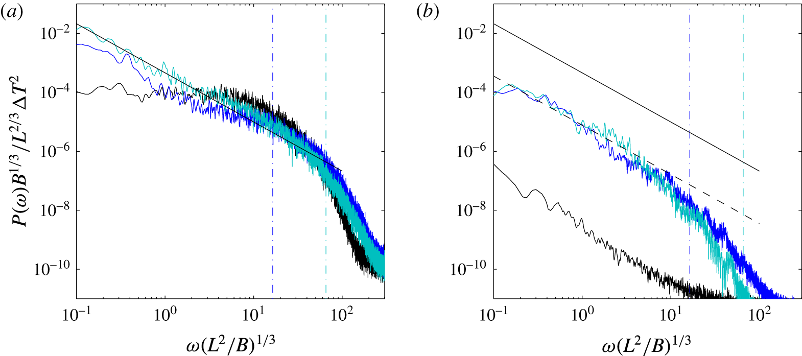
Under strong rotation (
 $Ro=5.6\times 10^{-3}$
, in the geostrophic boundary layer regime; blue lines in figure 16) the frequency spectrum in the boundary layer on the heated region of the base shows greater power at low frequencies
 $\unicode[STIX]{x1D714}<(B/L^{2})^{1/3}$
(which in this experiment corresponds to
 $\unicode[STIX]{x1D714}<0.03f$
), implying either an increased input of kinetic energy directly from available potential energy to motion at larger scales or an upscale transfer of kinetic energy from small to large length scales. There is also a decrease of power in the range
 $1<\unicode[STIX]{x1D714}(L^{2}/B)^{1/3}<30$
(
 $0.03f<\unicode[STIX]{x1D714}<f$
). The spectrum at
 $\unicode[STIX]{x1D714}<30(B/L^{2})^{1/3}$
(or
 $\unicode[STIX]{x1D714}<f$
) has slope close to
 $-5/3$
. From figure 16(a) the power in the boundary layer fluctuations at
 $\unicode[STIX]{x1D714}>30(B/L^{2})^{1/3}$
(which is also
 $\unicode[STIX]{x1D714}>f$
), and hence in small length scales, is not affected by rotation. In contrast, the spectrum of interior fluctuations above the heated base (figure 16
b) is greatly influenced by rotation, the power at frequencies less than
 $30(B/L^{2})^{1/3}$
increasing by three orders of magnitude at this Rossby number. Thus the geostrophic boundary layer regime involves a turbulent boundary layer in which only scales of motion much larger than the boundary layer thickness are controlled by rotation, along with an interior flow in which essentially all scales of variability are controlled by rotation. The temperature variability in the interior can be attributed largely to unsteadiness of the gyre circulations and to intermittent and migratory vortical plumes, which lead to much greater temperature variability in the interior in the rotating case, although the power remains approximately 30–50 times smaller than in the boundary layer. The
 $-5/3$
spectrum at low frequencies suggests upscale transfer of kinetic energy.
For the strongest rotation rate used in the experiments (
 $Ro=7.1\times 10^{-4}$
, in the chimney regime; cyan lines in figure 16) there was only a small additional increase in scalar fluctuation power in the boundary layer (somewhat uniformly by a factor of two at
 $\unicode[STIX]{x1D714}<30(B/L^{2})^{1/3}$
, or
 $\unicode[STIX]{x1D714}<0.1f$
) relative to the rotating case discussed above. The increase is likely due to the greater number of unsteady vortical plumes in the chimney regime, and to stronger coupling of the boundary layer and interior in the convective vortex flow. The boundary layer spectrum is again well described by the
 $-5/3$
power law over two orders of magnitude in frequency (in this case at
 $\unicode[STIX]{x1D714}<0.1f$
). In the interior above the heated base (figure 16
b) the spectrum for very strong rotation shows no significant difference from the geostrophic boundary layer regime excepting a small decrease of power at the largest frequencies. The data for the different rotation rates show that the temperature fluctuation statistics scale with the buoyancy frequency rather than with the inertial frequency.
9 Discussion
The regime diagram (figure 17) is created by matching the Nusselt number scalings across each of the transitions between the regimes outlined in § 2, except for the transition into the conduction regime, which is delineated by the disappearance of the thermal boundary layer,
 $\unicode[STIX]{x1D6FF}=H$
. The numerical prefactors for the transitions from non-rotating to geostrophic boundary layer and from geostrophic boundary layer to inertial chimney regimes were calculated from the fits of the scaling solutions to the experimental data in those regimes. As no empirical prefactors are available for the geostrophic chimney and conduction regimes, the prefactors have been set to one (transitions shown as broken lines). The locus of the transition from viscous to inertial non-rotating convection is similarly uncertain and is estimated from both the experiments of Mullarney et al. (Reference Mullarney, Griffiths and Hughes2004) and conversion of the transition found for the case of applied temperature difference (Gayen et al.
Reference Gayen, Griffiths and Hughes2014). We also regard the condition for transition from the non-rotating to the inertial chimney regime as uncertain, but hypothesise that it lies near the conditions for the horizontal flow to become organised into basin-scale gyres that promote formation of vortical plumes over much of the region of destabilising boundary flux, and therefore near the critical Rossby number
 $Ro_{crit}$
(2.20; dotted line).
Regime diagram based on the scaling solutions in § 2 plotted for
 $Pr=4.4$
,
 $A=0.16$
and
 $A_{y}=0.24$
. The experimental conditions from table 1 are shown (black circles) with non-rotating runs on the left-hand axis. For the two key transitions (non-rotating to geostrophic boundary layer to inertial chimney) the loci are plotted with numerical prefactors evaluated from the experiments. Transitions indicated with a broken line are less certain as a result of one or more unknown numerical prefactors (which are therefore set to one), and the dotted line indicates that the condition for transition is uncertain. Prefactors taken from § 6 are
 $c_{3}=0.47$
,
 $c_{6}=0.97$
,
 $c_{7}=1.45$
and
 $c_{9}=2\times 10^{-2}$
.
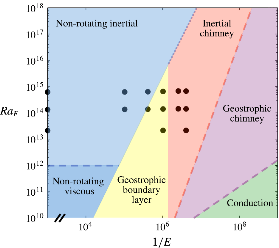
The experimental data span the non-rotating, geostrophic boundary layer and inertial chimney regimes. No empirical evidence is available for the geostrophic chimney regime (predicted to appear only at rotation rates beyond the practical limits set by curvature of the isopotential surfaces in the experiments), nor for the conduction regime predicted for very much faster rotation. The predicted regime boundaries are also dependent on the aspect ratios and Prandtl number, a factor to be considering when extrapolating the results to ocean parameter values. The boundary conditions too are likely to influence the regime boundaries, noting that the appropriate boundary conditions at the sea surface are a combination of imposed buoyancy flux (the radiative heat input), and temperature-dependent evaporative and sensible heat fluxes, all having smoother latitude dependence than the piecewise uniform conditions used in the experiments, along with a fixed minimum temperature due to freezing.
Rotating horizontal convection in the chimney regimes involves vortical convection within the chimney region and we have proposed (following Maxworthy & Narimousa Reference Maxworthy and Narimousa1994) that the two dominant regimes found in rotating Rayleigh–Bénard convection (Calkins et al. Reference Calkins, Julien, Tobias and Aurnou2015; Julien et al. Reference Julien, Aurnou, Calkins, Knobloch, Marti, Stellmach and Vasil2016; Plumley et al. Reference Plumley, Julien, Marti and Stellmach2016) have relevance to the chimney dynamics. At weak rotation or large Rayleigh numbers both Rayleigh–Bénard and the convection within the chimney region are dominated by local accelerations, with the heat transport independent of rotation, despite the columnar vortex structure. Under rapid rotation both Rayleigh–Bénard and the chimney in horizontal convection are dominated by geostrophic control at the plume scale. However, details such as the roles of Ekman pumping and the interaction of the plumes with the stable density stratification and mean flow warrant further investigation using direct numerical simulations of horizontal convection, allowing comparison with rotating Rayleigh–Bénard and the convection under temperature boundary conditions.
Finally, some comparison can be made with previous DNS of a rotating rectangular basin with an imposed temperature difference, in which heating and cooling temperatures were each uniform over one half of the base (Vreugdenhil et al.
Reference Vreugdenhil, Gayen and Griffiths2016). The observed flow structure is qualitatively the same, showing basin-scale gyres and cyclonic vertical plumes in a chimney region associated with the destabilising boundary heat flux. The chimney convection in both systems becomes a more prominent feature for larger rotation rates. The DNS results are also consistent with the geostrophic boundary layer scaling solution at
 $Ro\ll 1$
(or
 $QPr\gg 1$
) and give a consistent condition for the non-rotating to geostrophic transition. However, in that study the geostrophic boundary layer scaling appears to hold even for very small values of the Ekman number (
 $E\approx 6\times 10^{-8}$
) with no evidence of transition to the chimney regime at conditions where that regime is predicted by the equivalent scaling analysis for the case of applied temperature difference. Hence it is not clear whether the chimney-dominated regime occurs for piecewise uniform applied temperatures, and the existing DNS results are too sparse to resolve the question.
10 Conclusions
Laboratory experiments with horizontal convection in a rotating rectangular box, along with theoretical scaling, provide the condition for transition from the effectively non-rotating convection regime, for imposed buoyancy flux and basin scales large enough that the thermal boundary layer is turbulent, to a geostrophic boundary layer regime. This regime is equivalent to that previously predicted for a rotating annulus and utilised in an early conceptual description of circulation in an ocean basin. Measurements of the boundary layer thickness, volume transport, temperature differences and adjustment times in the geostrophic boundary layer regime are consistent with the scaling solution for convection dominated by geostrophic constraints on the basin-scale horizontal circulation within the thermal boundary layer. The regime is re-interpreted here as that in which the convection is controlled by the relative magnitude of horizontal advective and Coriolis accelerations. Under strong rotation, where the Ekman boundary layer transport becomes small, there is a simple dependence of the flow and temperature differences on the convective Rossby number
 $Ro$
(over the range
 $10^{-1}>Ro>10^{-3}$
) and the dynamics is no longer influenced by viscous stress or determined by the relative thickness of the Ekman and thermal boundary layers. Geostrophic flow inhibits transport, which becomes restricted to boundary currents and eddies, and gives Nusselt number values relative to the non-rotating case
 $Nu/Nu_{0}\sim Ro^{1/6}$
. While the transport is governed by the thermal boundary layer dynamics the time-averaged circulation throughout the box takes the form of a set of large gyres extending throughout the depth and having horizontal scales comparable to the box width.
When
 $E<10^{-6}$
(corresponding to
 $Ro<10^{-3}$
) for the value of Prandtl number and the basin geometry used here, the experiments show evidence for an inertial chimney regime, as is predicted for convective circulation controlled by vertical accelerations in a field of vortical plumes over the region of destabilising boundary heat flux. In this regime the local plume dynamics is similar to that predicted to hold in oceanic deep convection chimneys, with no dependence on rotation and boundary stress. Coupling of the non-rotating chimney dynamics to the basin-scale circulation and the diffusive boundary layer produced in the region of stabilising boundary heat flux does not change these aspects of the solution. We speculate that observed gyre structures in the measured circulation contribute to holding stable boundary layer water adjacent to the destabilising boundary flux for longer, and further from the end wall of the box, at larger rotation rates, thereby promoting stronger chimney convection removed from the end wall and side boundaries. The experiments do not reach conditions, at even stronger rotation relative to buoyancy forcing, for which a further chimney regime is predicted to involve convection controlled by geostrophic flow at the plume scale and heat transport returning to a dependence on rotation rate.
Acknowledgements
We thank T. Beasley, B. Tranter and A. Rummery for construction of equipment and laboratory assistance. We thank Dr A. Kiss for providing helpful comments on calculating the transport from horizontal velocity fields. The particle tracking velocimetry was analysed using Streams 2.01 software, for which we thank Dr R. Nokes. The research was supported by Australian Research Council grant DP140103706, C.A.V. was supported by an Australian Postgraduate Award granted by the Australian Government Research Training Program and B.G. was funded by an Australian Research Council Discovery Early Career Fellowship DE140100089.
Supplementary movies
Supplementary movies are available at https://doi.org/10.1017/jfm.2017.249.
Appendix A. Effects of curvature of isopotential surfaces
Surfaces of constant potential owing to the centrifugal acceleration are paraboloidal surfaces centred on the axis of rotation. The surfaces are described by
 $\unicode[STIX]{x1D702}-\unicode[STIX]{x1D702}_{0}=f^{2}r^{2}/8g$
, where
 $\unicode[STIX]{x1D702}_{0}$
is the height of a potential surface at the axis and
 $r$
is the radius about the axis. The height differences across the box width
 $W$
are small compared to those along the length of the box and the maximum difference is characterised by
 $\unicode[STIX]{x1D702}(r=L/2)-\unicode[STIX]{x1D702}(0)=f^{2}L^{2}/32g$
.
Through buoyancy-driven flow the top of the thermal boundary layer tends to relax toward an isopotential surface (a planar and horizontal surface in the non-rotating case). Geostrophic balance maintains lateral gradients in boundary layer thickness. However, if it is assumed that on averaging across the box width
 $W$
the top of the boundary layer remains approximated by an isopotential surface, then the parabolic shape of the surface represents a physical barrier to flow of the coldest boundary layer water, equivalent to the bottom boundary being higher at the mid-section of the box (
 $x=0$
) than at the ends. The coldest water will tend to accumulate near the cooled end, and the boundary layer will be thicker near the cooled end and thinner at the mid-section.
The measured boundary layer thickness can be expressed as
 $\unicode[STIX]{x1D6FF}(x)=\unicode[STIX]{x1D6FF}_{n}+f^{2}(x-L/2)^{2}/8g$
, where the geostrophic boundary layer scaling (2.15) gives
 $\unicode[STIX]{x1D6FF}_{n}/L\sim (Ra_{F}E/A_{y})^{-1/4}$
. Writing the centrifugal term as a function of the Ekman number gives for the geostrophic boundary layer regime
 $$\begin{eqnarray}\unicode[STIX]{x1D6FF}_{g}(x)/L\approx c_{4}(Ra_{F}E/A_{y})^{-1/4}+(\unicode[STIX]{x1D708}^{2}/8gL^{3})(x/L-1/2)^{2}E^{-2}.\end{eqnarray}$$
Normalising (A 1) by the non-rotating scaling (2.10) and expressing the result in terms of the Rossby number,
 $$\begin{eqnarray}\unicode[STIX]{x1D6FF}_{g}(x)/\unicode[STIX]{x1D6FF}_{0}\approx c_{6}A_{y}^{1/4}Ro^{-1/6}+c_{2}^{-1}(\unicode[STIX]{x1D708}^{2}/8gL^{3})(x/L-1/2)^{2}(Ra_{F}^{5}Pr^{-7}Ro^{-8})^{1/6}.\end{eqnarray}$$
The adjustment time scale (4.3) is predicted to be dependent on the average boundary layer thickness over the cooled region. Hence a correction to (4.3) for isopotential curvature gives
 $$\begin{eqnarray}\unicode[STIX]{x1D70F}_{g}/\unicode[STIX]{x1D70F}_{0}\approx c_{10}A_{y}^{1/4}Ro^{-1/6}+c_{2}^{-1}(\unicode[STIX]{x1D708}^{2}/96gL^{3})(Ra_{F}^{5}Pr^{-7}Ro^{-8})^{1/6}.\end{eqnarray}$$
The heat transport through the boundary layer is fixed by the imposed boundary flux and the Nusselt number is given by
 $Nu\sim L/\overline{\unicode[STIX]{x1D6FF}}$
, where
 $\overline{\unicode[STIX]{x1D6FF}}$
is the thermal boundary layer thickness averaged over the cooled region. For the geostrophic boundary layer regime the predicted Nusselt number (2.18) with centrifugal correction becomes
 $$\begin{eqnarray}Nu/Nu_{0}\approx c_{7}/(A_{y}^{1/4}Ro^{-1/6}+c_{3}c_{7}^{-1}(\unicode[STIX]{x1D708}^{2}/96gL^{3})(Ra_{F}^{5}Pr^{-7}Ro^{-8})^{1/6}).\end{eqnarray}$$
Appendix B. Ekman correction to the geostrophic boundary layer
With rotation the boundary friction at the base is apparent only within an Ekman layer, which is thinner than the thermal boundary layer for
 $Q>1$
. For
 $Q\sim O(1)$
, or weak rotation, the Ekman layer contributes to the total mass and heat transport. Following the assumption of Park & Whitehead (Reference Park and Whitehead1999) that the Ekman layer transport is separable from the buoyancy-forced transport of the thermal boundary layer, the corrected scaling for the Nusselt number (adding the Ekman layer contribution to (2.15), expressing in terms of
 $Ro$
and normalising by the non-rotating scaling (2.10)) becomes
 $$\begin{eqnarray}Nu/Nu_{0}\approx c_{7}A_{y}^{-1/4}Ro^{1/6}/(1+\sqrt{2}c_{4}^{-1}(RoPr)^{1/2}A_{y}^{-1/4}).\end{eqnarray}$$



