Researchers in a wide variety of fields including political science regularly employ the Cox proportional hazards model to analyze duration data. This popularity has given rise to a robust literature of simulation studies that assess the Cox model and its properties and provide crucial guidance to applied researchers tasked with choosing between the many options available for conducting duration analyses (e.g., Chastang, Byar and Piantadosi Reference Chastang, Byar and Piantadosi1988; Keele Reference Keele2010; Desmarais and Harden Reference Desmarais and Harden2012; Box-Steffensmeier, Linn and Smidt Reference Box-Steffensmeier, Linn and Smidt2014; Benaglia, Jackson and Sharples Reference Benaglia, Jackson and Sharples2015; Kropko and Harden Reference Kropko and Harden2018).Footnote 1 A critical component of these simulation studies is generating durations conditional on covariates and their corresponding coefficients. Typical methods for generating these durations often employ known distributions—such as the exponential, Weibull, or Gompertz—that imply specific shapes for the baseline hazard function. This approach is potentially problematic because it contradicts a key advantage of the Cox model—the ability to leave the distribution of the baseline hazard unspecified. By restricting the simulated data to a known (usually parametric) form, these studies impose an assumption that is not required in applications of the Cox model. In practice the baseline hazard can exhibit considerable heterogeneity, both across the many fields which employ the Cox model and within a given field (see Cox et al. Reference Cox, Chu, Schneider and Munoz2007). Thus, simulating durations from one specific parametric distribution may not adequately approximate the data that many applied researchers analyze, reducing the simulation’s generalizability. Furthermore, in studies that compare parametric estimators to the Cox model, this approach could bias results in favor of the parametric estimators.
Here we address these problems by introducing a novel method for simulating durations without specifying a particular distribution for the baseline hazard function. The method first generates a cumulative distribution function (CDF) of event occurrence (i.e., failure) from randomly drawn points. It then uses this function to generate other baseline functions, including the baseline hazard. Because it randomly generates the failure CDF, the method can produce a wide variety of shapes for the baseline hazard. This heterogeneity matches the Cox model’s inherent flexibility. By remaining agnostic about the distribution of the baseline hazard, our method better constructs the assumed data generating process (DGP) of the Cox model. Moreover, repeating this process over many iterations—in a single simulation or across multiple simulations with varying conditions—yields more variation in the simulated samples, which is consistent with the wide variety of data that applied researchers analyze with the Cox model.
BACKGROUND
Several researchers have considered the problem of simulating durations for the Cox model over the last several decades. The Cox model is defined in terms of its hazard function:
 $$h\left( {t\!\mid\,\!X} \right)\,{\equals}\,h_{0} \left( t \right)\,\exp \left( {X\,\beta } \right).$$
Here X represents the model covariates, β represents the corresponding regression coefficients, and h 0(t) represents the baseline hazard, or the hazard when X=0. The cumulative baseline hazard function is defined as
 $$H_{0} \left( t \right)\,{\equals}\,{\int}_0^t {h_{0} \left( s \right)\,ds} ,$$
the failure CDF is
 $$F_{0} \left( {t\left| X \right.} \right)\,{\equals}\,1{\minus}\exp \left[ {{\minus}H_{0} \left( t \right)\,\exp \left( {X\,\beta } \right)} \right],$$
and the baseline survivor function is
 $$S_{0} \left( {t\left| X \right.} \right)\,{\equals}\,\exp \left[ {{\minus}H_{0} \left( t \right)\,\exp \left( {X\,\beta } \right)} \right].$$
Leemis (Reference Leemis1987) demonstrated that durations can be drawn from the assumed DGP of a variety of survival models by applying the inverse of the cumulative hazard function
 $\left( {H_{0}^{{{\minus}1}} } \right)$
to random draws from a uniform distribution on the [0, 1] interval (see also Leemis, Shih and Reynertson Reference Leemis, Shih and Reynertson1990; Shih and Leemis Reference Shih and Leemis1993; Bender, Augustin and Blettner Reference Bender, Augustin and Blettner2005). Let u be a random draw from a
 ${\bf {\cal U}} \left[ {0,\,1} \right]$
. From equation (3), a duration, E, can be drawn at random by computing
 $$E\,{\equals}\,H_{0}^{{{\minus}1}} \left[ {{\minus}\log \left( u \right)\,\exp \left( {{\minus}X\,\beta } \right)} \right].$$
If the cumulative baseline hazard function can be inverted, these random draws can be converted into simulated durations (Bender, Augustin and Blettner Reference Bender, Augustin and Blettner2005, 1716–7).
Others have pointed out that the method of inverting the cumulative baseline hazard is problematic (though not impossible to use) when trying to generate durations with time-varying covariates (Sylvestre and Abrahamowicz Reference Sylvestre and Abrahamowicz2008; Austin Reference Austin2012). Building on those studies, Crowther and Lambert (Reference Crowther and Lambert2013) developed a method for generating durations using complex parametric distributions for the baseline hazard. Hendry (Reference Hendry2014) proposed a method of generating durations that simulates from a truncated piecewise exponential distribution (see also Zhou Reference Zhou2001). Overall, this work provides several useful options to generate durations for simulation studies involving the Cox model. However, one shortcoming common among them is the reliance on a known, parametric distribution of some kind. Importantly, this choice also appears in actual simulation studies that assess the Cox model’s properties, including recent examples from political science (e.g., Desmarais and Harden Reference Desmarais and Harden2012; Box-Steffensmeier, Linn and Smidt Reference Box-Steffensmeier, Linn and Smidt2014).
Simulation studies should seek to generate “plausible” data so that results can be generalized to data sets collected by applied researchers across and within the fields that employ the method in question (Crowther and Lambert Reference Crowther and Lambert2013). While using a known distribution may be reasonable for the goals of some simulations, it may also be too restrictive in others. Indeed, a major feature of the Cox model that makes it a popular choice is its flexibility with respect to the distributional form of the baseline hazard. Moreover, consider a simulation in which researchers wish to compare the performance of the Cox model to that of a parametric model (e.g., Chastang, Byar and Piantadosi Reference Chastang, Byar and Piantadosi1988; Benaglia, Jackson and Sharples Reference Benaglia, Jackson and Sharples2015; Kropko and Harden Reference Kropko and Harden2018). Simulating durations from the parametric model’s assumed distribution will artificially inflate the performance of the parametric model because that model’s assumption about the true DGP is correct. This practice may be problematic if real data do not come from that distribution.
In short, simulation from a known, parametric distribution may not provide the most realistic data conditions in which to conduct simulation studies of the Cox model. Below we introduce a method that addresses this problem by generating durations that do not correspond to a specific functional form for hazard. This approach better matches the assumptions (or lack thereof) of the Cox model.
SIMULATING DURATIONS
The central task in simulation studies of the Cox model is to generate data in which the analyst knows the DGP (i.e., the correct specification of covariates and true values of the coefficients), and thus can compare the Cox model’s estimates to the truth. As mentioned above, a challenge in this process is to simulate data that could reasonably be generated in nature so that the simulation study provides a useful approximation of an applied research setting. In the case of the Cox model, the shape of the baseline hazard is a crucial part of addressing this challenge. The Cox model does not assume a particular shape; thus, for the simulation to match the flexibility of the Cox model, it should not depend on a particular shape when generating durations.
Accordingly, in what follows we describe what we call the random spline method for simulating Cox model data. Using this method, the durations come from a randomly generated baseline hazard. The random spline method gives the analyst control over the correct covariates and true values of the coefficients, but does not restrict the baseline hazard to a known distributional form. More specifically, it involves fitting a cubic spline to randomly selected points to create the failure CDF, then forming a baseline hazard function from this CDF from which to draw durations. The method also gives the analyst considerable control over several features of this process. We describe the steps to the method below. A function in the R package coxed implements the method with several options for user control.
Generating the Baseline Hazard Function
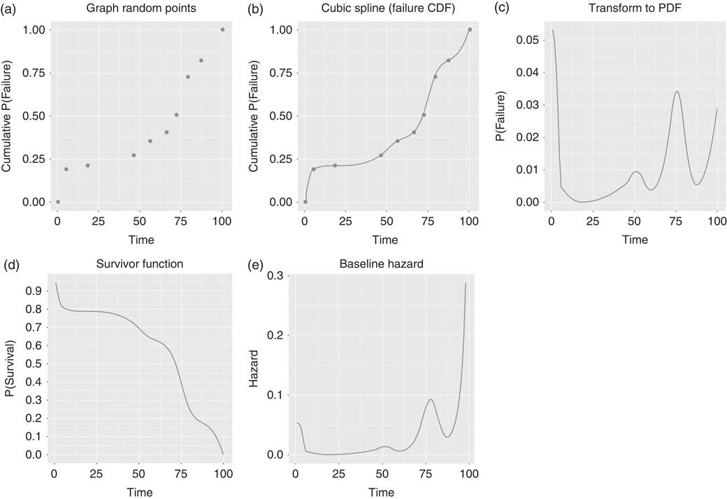
The first step is to randomly generate a failure CDF. To do so it is necessary to create a time index of length T and set that index as the x-axis on a graph. Without loss of generality, we select the integers from 1 to 100 (T=100) for this explanation. Next, we draw k points, where
 $k\,\ll\,T$
. Here we select k=10. The x-coordinates for two of the k points are the minimum and maximum of the time index (1 and 100 in this case). Then we randomly draw x-coordinates for the other k−2 points from the remaining time points with uniform probability. With our x-coordinates in place, we then set the y-coordinate for the point at the minimum time to be 0, we set the y-coordinate for the point at the maximum time to be 1, and we randomly draw y-coordinates for the other k−2 points from a
 ${\bf {\cal U}} \left[ {0,\,1} \right]$
. We sort those coordinates in ascending order (because a CDF must be non-decreasing), then graph them (see Figure 1(a)).Footnote
2
Generating a baseline hazard function via the random spline method Note: (a) An example of the randomly-drawn time points. (b) The cubic spline fit to those points to create the failure cumulative distribution function (CDF). (c) The transformation from the failure CDF to a failure probability density function (PDF). (d) Plots the survivor function and (e) graphs the baseline hazard function.
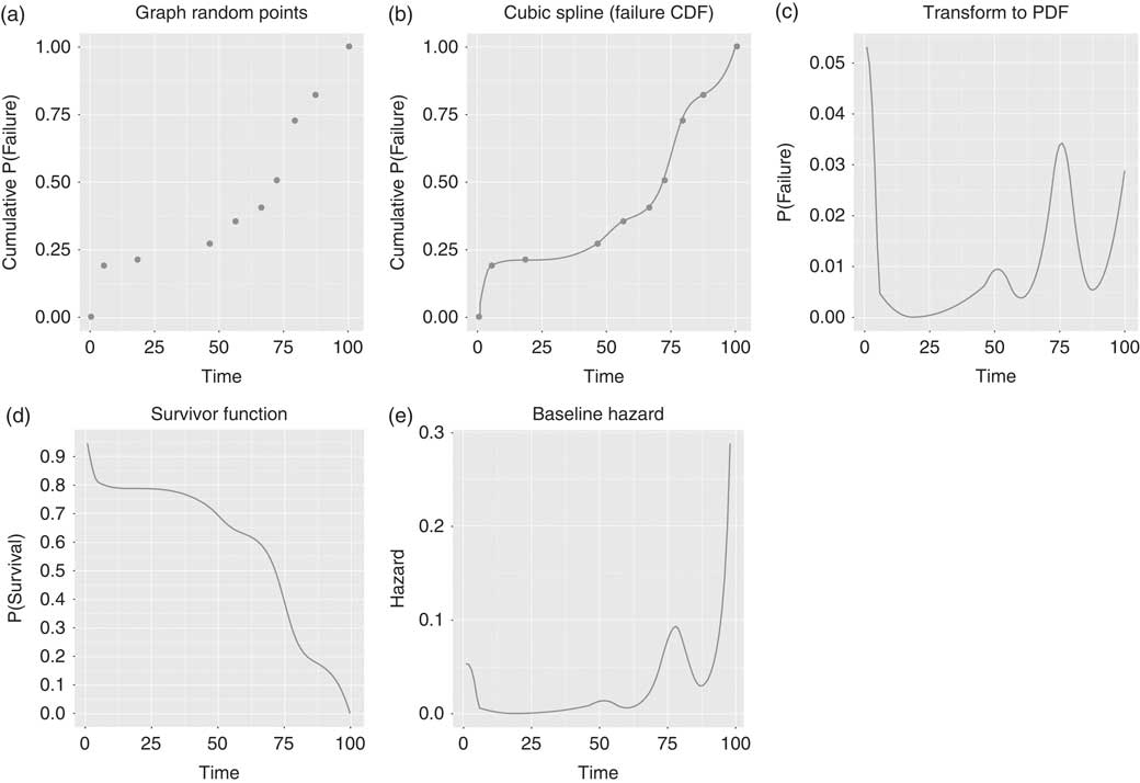
After graphing the points we construct the failure CDF by fitting a cubic smoothing spline—a piecewise function that connects the k points through a series of third-order polynomials—as shown in Figure 1(b). We employ Hyman’s (Reference Hyman1983) cubic smoothing function because it preserves the CDF’s monotonicity. Next we construct the failure time density function (PDF) by computing the first differences of the CDF at each time point (Figure 1(c)). We generate the survivor function by subtracting the failure CDF from 1 (Figure 1(d)). Finally, we compute the baseline hazard by dividing the failure PDF by the survivor function (Figure 1(e)).
Generating Durations
Having generated the baseline failure CDF, the baseline survivor function, and the baseline hazard function, our next task is to generate individual durations from this function in a way that depends on analyst-controlled covariates and coefficient values. First, we randomly generate p covariates, which are column vectors of length equal to the sample size, N. We also define true values for the p coefficients corresponding to those covariates. We then create linear predictor values by multiplying the matrix of the covariates, X , by the vector of coefficients, β . Having generated the systematic component of the model, we next use the baseline survivor function in equation (4) and the linear predictor to construct the individual-specific survivor functions (Box-Steffensmeier and Jones Reference Box-Steffensmeier and Jones2004, 65):
 $$S_{i} \left( t \right)\,{\equals}\,S_{0} \left( t \right)^{{\exp ({\bf X}_{i} {\bf \beta })}} .$$
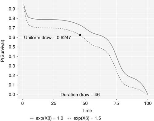
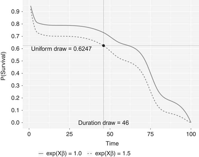
In other words, we take the baseline survivor function to the power of each element of exp( Xβ ). If, for example, N=500, then exp( Xβ ) has 500 elements and the baseline survivor function is taken to the power of each of these elements to produce 500 individual-specific survivor functions. For example, in Figure 2, we consider one observation with the property that exp( Xβ )=1.5, so that the risk of failure at time t conditional on survival through time t is 50 percent higher than the baseline. This observation’s survivor function is the dashed line and the solid line is the baseline survivor function.
Drawing a duration for an observation from the simulated survivor function Note: The solid line is the baseline survivor function, which represents the survival probability for an observation with a 0 for every covariate. The dashed line is the survivor function for an observation whose exponentiated linear predictor is 1.5. This observation has a risk of failure at time t conditional on survival through time t that is 50 percent higher than the baseline.
Next, for each observation, we randomly draw one value from the
 ${\bf {\cal U}} \left[ {0,\,1} \right]$
distribution. We then calculate the time point at which each individual observation’s survivor function becomes less than this random uniform draw. These time points are the simulated durations for the observations. For example, in Figure 2, we randomly draw a value of 0.6247 from the
 ${\bf {\cal U}} \left[ {0,\,1} \right]$
distribution, which we mark with a horizontal line. The observation’s survivor function, the dashed line, intersects this horizontal line at 46 on the x-axis. Thus, the duration that we draw for this observation is t=46.
We draw a duration in this way for all N observations. The result is a vector of durations generated according to known covariates and coefficient values but an arbitrary baseline hazard function. Finally, the analyst may wish to censor some observations according to some process of interest. For example, censored observations could be selected randomly with a uniform or other distribution (e.g., Sylvestre and Abrahamowicz Reference Sylvestre and Abrahamowicz2008; Hendry Reference Hendry2014). This would conform to the Cox model’s assumption that, conditional on the covariates, the censoring mechanism is independent of the DGP that produces the durations (Jackson et al. Reference Jackson, White, Seaman, Evans, Baisley and Carpenter2014). Alternatively, the analyst may wish to simulate data with violations to this assumption to observe the consequences for the estimates.Footnote 3
The durations and the generated covariates together form a simulated data set. The analyst could make changes to the DGP in several ways, such as adding measurement error to a covariate. Importantly, the shape of the baseline hazard function can vary considerably, although the analyst can choose whether to keep that function fixed across the entire simulation or allow it to vary at every iteration. The variation in the (potential) shapes of the simulated baseline hazard reflects the heterogeneity found in real data across the many disciplines that employ the Cox model. We contend that allowing such heterogeneity increases the generalizability of the analyst’s simulation results.
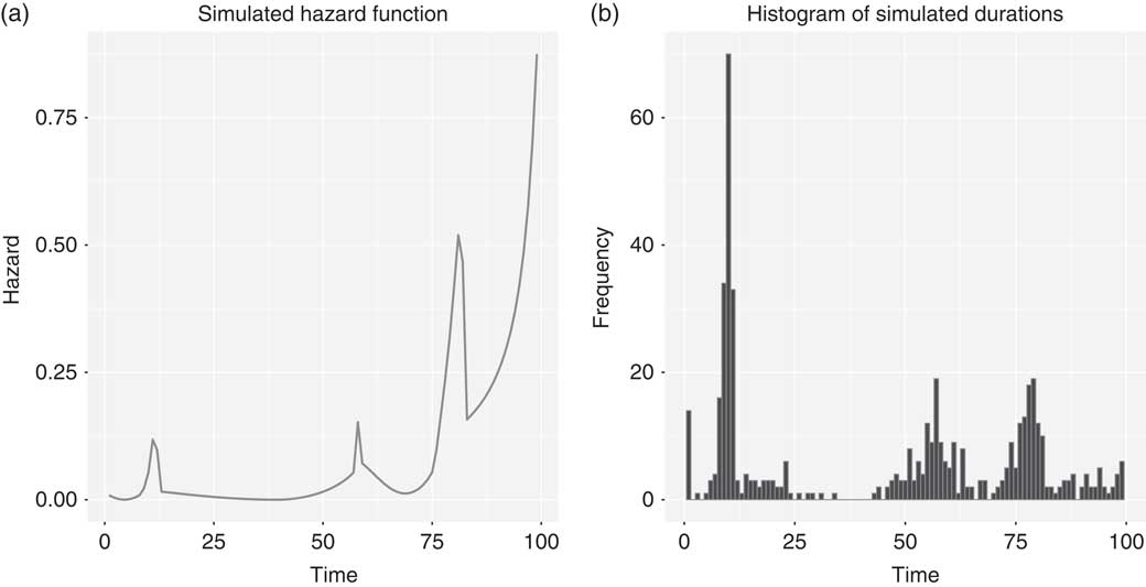
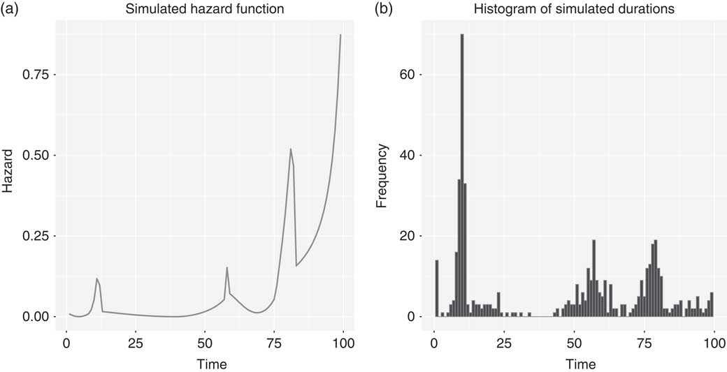
Figure 3 shows an example of one simulated dataset generated with the random spline method (T=100, k=10, N=500, and p=3). The graph in Figure 3(a) plots the baseline hazard function. Figure 3(b) gives a histogram of a sample of durations simulated from that hazard function.
Example output from the random spline method Note: The graphs illustrate output from one iteration of the random spline method. (a) The hazard function and (b) a sample of durations generated from the hazard function.
Simulation Example with the Random Spline Method
Here we illustrate the random spline method with an example simulation of 1000 data sets, which we use to compare the Cox model to two parametric estimators. We set the same simulation parameters as in Figure 3: T=100, k=10, N=500, and p=3. We generate the covariates from normal distributions, though this is an arbitrary choice. The true parameter values on these variables are, respectively, β 1=0.50, β 2=−0.50, and β 3=0.75.Footnote 4 We use the random spline method to generate a single baseline hazard that is used at every iteration of the simulation. However, an option in the R function allows the analyst to generate a new baseline hazard using the same parameters at each iteration. We randomly select 5 percent of the observations with uniform probability and code them as right-censored. At each iteration we estimate an exponential model, Weibull model, and a Cox model.Footnote 5 We monitor each estimator’s coefficient estimates in proportional hazards parameterization and the root mean squared error (RMSE) of those estimates.
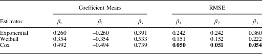
Table 1 gives the results for each estimator. The left columns report the means of the coefficient estimates across the simulated data sets for each estimator (in proportional hazards parameterization). The right columns give coefficient RMSE values. Bold entries indicate the estimator with the lowest RMSE for each coefficient.
Coefficient Estimate Means and Root Mean Squared Error (RMSE) From Data Simulated Via the Random Spline Method

Note: Cell entries report coefficient estimate means and RMSE for the exponential, Weibull, and Cox model estimates (in proportional hazards parameterization). True coefficient values are β 1=0.50, β 2=−0.50, and β 3=0.75. Bold entries indicate the estimator with the lowest RMSE for each coefficient. N=500 in all simulations.
The coefficient means indicate that the exponential and Weibull models are biased, while the Cox model returns estimates that are, on average, very close to the true values set in the DGP. The RMSEs also show that the Cox model performs the best of the three estimators; it produces the lowest values for all three coefficients. The Weibull model, which does not assume a flat baseline hazard, consistently outperforms the exponential model with respect to RMSE. Overall, the results conform to expectations. The random spline method produces a baseline hazard that violates the assumptions of the exponential and Weibull models. The violations have negative consequences for the estimates from the parametric models (especially those from the exponential model), but do not affect the Cox model estimates. This is a clear indication that the random spline method simulates durations that conform to the assumed DGP of the Cox model, but not the DGP of any particular parametric model.
CONCLUSIONS
Simulation studies are critical for understanding and developing statistical methods because they give the analyst precise control over the DGP. However, for these studies to be generalizable, simulated data should match the assumptions of the estimator of interest and accurately reflect data that researchers might collect in the field. This is particularly difficult when simulating data for the Cox proportional hazards model. Due to its semi-parametric estimation method, the Cox model does not assume a shape for the baseline hazard function and cannot be used directly to draw simulated durations. Researchers can simulate data from the distribution implied by a parametric estimator or other known distribution, but this approach is inconsistent with the Cox model’s flexibility, may not produce realistic data, and could bias simulation results in favor of a parametric estimator.
To address this problem, we demonstrate a method for generating durations that does not rely on a specific distributional form. Instead, it constructs a failure CDF at random, then produces durations based on the baseline hazard implied by that function. This approach approximates a wide variety of possible data sets that applied researchers might collect and matches the flexibility of the Cox model. The method provides researchers with a means of generating durations for simulation studies without restricting the DGP to a specific distribution. Furthermore, our implementation in R is quite flexible, allowing researchers to program a variety of different conditions that may arise in applied settings into their simulations. We expect that the random spline method can improve simulation studies of duration models, allowing applied researchers to learn more from them and make better choices in employing duration models in their work.