







1. Introduction
Wall-bounded turbulent flows over rough surfaces are among the most common examples of turbulent flows found in nature and engineering. Examples include pipe flows (e.g. Langelandsvik, Kunkel & Smits Reference Langelandsvik, Kunkel and Smits2008), geophysical flows (e.g. Lin et al. Reference Lin, Moeng, Sullivan and McWilliams1997), flows around ships (e.g. Schultz Reference Schultz2007), aircraft (e.g. Kundu, Raghunathan & Cooper Reference Kundu, Raghunathan and Cooper2000) and re-entry vehicles (e.g. Finson & Clarke Reference Finson and Clarke1980), flows within turbomachinery (e.g. Bons et al. Reference Bons, Taylor, McClain and Rivir2001), etc. The characteristics of turbulent flows over hydraulically rough surfaces are significantly different than for flows over surfaces that are considered hydraulically smooth, with the mechanisms responsible for these characteristics exhibiting strong dependence on the roughness geometry. Observed effects of surface roughness on wall-bounded turbulent flows include increased wall shear stress (Cardillo et al. Reference Cardillo, Chen, Araya, Newman, Jansen and Castillo2013), modification of the energy spectrum (Hong, Katz & Schultz Reference Hong, Katz and Schultz2011) and length scales (Cardillo et al. Reference Cardillo, Chen, Araya, Newman, Jansen and Castillo2013) of turbulence, creation of additional vortical structures (Ikeda & Durbin Reference Ikeda and Durbin2007), modification of velocity and Reynolds stress profiles (Krogstad, Antonia & Browne Reference Krogstad, Antonia and Browne1992; Krogstadt & Antonia Reference Krogstadt and Antonia1999; Keirsbulck et al. Reference Keirsbulck, Labraga, Mazouz and Tournier2002; Lee & Sung Reference Lee and Sung2007; Burattini et al. Reference Burattini, Leonardi, Orlandi and Antonia2008; Cardillo et al. Reference Cardillo, Chen, Araya, Newman, Jansen and Castillo2013) and changes to turbulent kinetic energy production (Ikeda & Durbin Reference Ikeda and Durbin2007; Burattini et al. Reference Burattini, Leonardi, Orlandi and Antonia2008).
The earliest effort to understand the effects of surface roughness can be traced back to the pipe flow measurements of Nikuradse (Reference Nikuradse1933). These experiments were used to characterise the dependence of wall shear stress,  $\tau _w$, based on a uniform sand grain roughness height. To make the effects of wall roughness widely available to the scientific and engineering community, Moody (Reference Moody1944), continuing the work of Colebrook (Reference Colebrook1939), developed the Moody chart to predict pressure losses in smooth and rough pipe flows. The ensuing years saw a significant effort aimed at characterising and understanding the effects of arbitrary surface roughness on the scaling of the profile for the mean streamwise velocity component,
 $\bar {u}$, as a function of distance from the wall,
 $y$. Here the overline is used to indicate a time-averaged quantity. As with smooth-walled flows, the mean velocity profile is commonly expressed using inner scaling, which reflects dependence on the wall shear stress,
 $\tau _w$, and kinematic viscosity,
 $\nu$. The velocity scale for inner scaling is therefore
 $u_\tau =(\tau _w/\rho )^{1/2}$, and the length scale is
 $\nu /u_\tau$, with
 $\rho$ being the density of the fluid. Throughout this article quantities scaled using these inner variables will be expressed using a superscripted
 $+$, for example
 $\bar {u}^{+}=\bar {u}/u_\tau$ and
 $y^{+}=yu_\tau /\nu$.
For flows over rough walls where the roughness height exceeds the depth of the corresponding smooth-walled viscous sublayer thickness, there exists a ‘roughness sublayer’ containing the dynamics of the roughness elements. Outside the roughness sublayer, the effect of the roughness is contained within the enhancement of  $\tau _w$ and the mean profile follows the inner-scaled mean velocity scaling of Clauser (Reference Clauser1954) and Hama (Reference Hama1954). They found independently, and almost simultaneously, that the mean velocity profile could be described using a modification to the log law in the form of
 \begin{equation} \bar{u}^{+} = \kappa ^{{-}1} \ln\left(y^{+}-y_0^{+}\right) + B + \varPi \kappa ^{{-}1} W(y/\delta) - \Delta U^{+}. \end{equation}
In (1.1),  $\kappa$ is the Kármán constant and
 $B$ is an additive constant. The outer-layer contribution to the mean flow is represented through profile parameter
 $\varPi$ and wake function
 $W(y/\delta )$ (Coles Reference Coles1956). Here
 $\delta$ indicates the thickness of the wall-bounded flow. The impact of surface roughness to the mean flow is introduced through the roughness function
 $\Delta U^{+}$ and
 $y_0^{+}$, the roughness offset which preserves the logarithmic scaling. For fully rough flows, i.e. for flows where the skin-friction coefficient plateaus (becomes essentially constant), the roughness function for uniform sand-grain roughness was found to be
 \begin{equation} \Delta U ^{+}=\kappa^{{-}1}\ln k^{+}+B-B', \end{equation}
where  $k$ is the roughness height and
 $B'$ is a constant for fully rough flow. Arising from Nikuradse (Reference Nikuradse1933), the behaviour of the mean streamwise velocity in the log layer for sand-grain roughness,
 $k_s$, was found to be
 \begin{equation} \bar{u}^{+} = \kappa^{{-}1}\ln{\frac{y}{k_s}} + 8.5, \end{equation}
leading to  $B'= 8.5$. An in-depth discussion of the various factors affecting
 $\Delta U^{+}$ can be found in the recent review article by Chung et al. (Reference Chung, Hutchins, Schultz and Flack2021).
Despite the roughness function providing some characterisation of the rough surface, it fails to be universally valid across different roughness types (Schultz & Flack Reference Schultz and Flack2009; Flack & Schultz Reference Flack and Schultz2014). Schultz & Flack (Reference Schultz and Flack2009) have characterised this non-universality based on a functional relation given by
 \begin{equation} \Delta U^{+} = f(k^{+}), \end{equation}
where  $f$ depends on both the nature of the roughness and the Reynolds number and can vary among different roughness types especially when studying flows in the transitionally rough regime. Hence, it is common to characterise a surface using its ‘equivalent sand grain roughness’,
 $k_s$, which is the value of
 $k$ that results in the mean velocity profile following (1.1), (1.2) and (1.3). For transitionally rough flow, the dependence of mean properties on the roughness geometry is particularly exacerbated, as the transition between viscous and pressure drag on the roughness elements is highly dependent on the element geometry.
For turbulence statistics, Townsend (Reference Townsend1976) hypothesised that for sufficiently high Reynolds numbers, the roughness-geometry-dependent behaviour is confined to within a few roughness heights of the wall and the flow in the outer region scales following smooth-wall scaling. Raupach, Antonia & Rjagopalan (Reference Raupach, Antonia and Rjagopalan1991) and Jiménez (Reference Jiménez2004) provide good reviews of the effects of surface roughness on turbulent flows while providing support for Townsend's outer-layer similarity hypothesis. Several experimental (e.g. Perry, Lim & Henbest Reference Perry, Lim and Henbest1987; Schultz & Flack Reference Schultz and Flack2003; Bakken et al. Reference Bakken, Krogstad, Ashrafian and Andersson2005; Connelly, Schultz & Flack Reference Connelly, Schultz and Flack2006; Kunkel & Marusic Reference Kunkel and Marusic2006; Schultz & Flack Reference Schultz and Flack2007) as well as numerical studies (e.g. Lee Reference Lee2002; Ashrafian, Andersson & Manhart Reference Ashrafian, Andersson and Manhart2004; Ashrafian & Andersson Reference Ashrafian and Andersson2006a, Reference Ashrafian and Anderssonb; Ikeda & Durbin Reference Ikeda and Durbin2007; Burattini et al. Reference Burattini, Leonardi, Orlandi and Antonia2008) have shown agreement with Townsend's outer-layer similarity hypothesis for boundary layer, pipe and channel flows. However, several studies have also shown that the effects of wall roughness can be found in the outer layer (e.g. Brzek et al. Reference Brzek, Cal, Johansson and Castillo2008; Cal et al. Reference Cal, Brzek, Johansson and Castillo2009; Hong et al. Reference Hong, Katz and Schultz2011; Cardillo et al. Reference Cardillo, Chen, Araya, Newman, Jansen and Castillo2013), particularly within the behaviour of the turbulence itself, providing evidence that roughness does indeed affect the flow in the outer layer. In some cases (e.g. Krogstad et al. Reference Krogstad, Antonia and Browne1992; Krogstadt & Antonia Reference Krogstadt and Antonia1999; Keirsbulck et al. Reference Keirsbulck, Labraga, Mazouz and Tournier2002; Smalley et al. Reference Smalley, Leonardi, Antonia, Djenidi and Orlandi2002; Leonardi et al. Reference Leonardi, Orlandi, Smalley, Djenidi and Antonia2003; Lee & Sung Reference Lee and Sung2007) evidence has been presented showing the non-universality of Townsend's outer-layer similarity hypothesis.
Amongst the observations contradicting Townsend's outer-layer similarity hypothesis are those of Hong et al. (Reference Hong, Katz and Schultz2011) who found that traces of roughness effects in the outer layer can be found through propagation of roughness-length scaled eddies from the inner layer. Cardillo et al. (Reference Cardillo, Chen, Araya, Newman, Jansen and Castillo2013) also comment on the influence of the roughness extending well beyond the inner region of boundary layer flow. Effects of roughness were visible in the outer layer for the turbulent stress tensor as found by Lee & Sung (Reference Lee and Sung2007). However, there was a smaller effect on the anisotropic stress tensor in the outer layer with the same trend observed for third-order moments of the velocity fluctuations as well. In contrast, experimental studies from Krogstadt & Antonia (Reference Krogstadt and Antonia1999) and Keirsbulck et al. (Reference Keirsbulck, Labraga, Mazouz and Tournier2002) show significant changes in the Reynolds stress tensor within turbulent boundary layer flows over rough walls.
Jiménez (Reference Jiménez2004) noted that in many cases, the non-conformity of these flows with Taylor's hypothesis was dependent on the ratio of the roughness height to that of the boundary layer thickness, specifically dependent on whether or not  $k$ protruded into the outer-scaled region, suggesting that
 $k/\delta$ should be less than
 $1/50$. Brzek et al. (Reference Brzek, Cal, Johansson and Castillo2008) postulated that in the case that the scale separation is not large, a mesolayer can be found between the inner and outer layers. This mesolayer diminishes with increasing Reynolds number but at lower Reynolds numbers can lead to the propagation of the viscous stresses from the inner layer to the outer layer. It was also hypothesised that in addition to having a small roughness height when compared with the boundary layer height, the momentum thickness Reynolds number must be greater than
 $10\,000$ for Townsend's outer-layer similarity hypothesis to be valid.
Another topic of debate is the choice of the appropriate length scale associated with the wall roughness. While Jiménez (Reference Jiménez2004) proposed the use of the ratio of roughness height to that of the boundary layer thickness,  $k/\delta$, Flack, Schultz & Shapiro (Reference Flack, Schultz and Shapiro2005) and Schultz & Flack (Reference Schultz and Flack2005) suggest using the ratio of the effective sand grain roughness to that of the boundary layer thickness,
 $k_s/\delta$. More recently, efforts are being made to quantify the effects of three-dimensional (e.g. MacDonald et al. Reference MacDonald, Chan, Chung, Hutchins and Ooi2016; Wu, Christensen & Pantano Reference Wu, Christensen and Pantano2020) and increasingly irregular roughness on turbulent flows (e.g. Busse, Lützner & Sandham Reference Busse, Lützner and Sandham2015; Busse, Thakkar & Sandham Reference Busse, Thakkar and Sandham2017; Forooghi et al. Reference Forooghi, Stroh, Magagnato, Jakirlić and Frohnapfel2017; Pathikonda & Christensen Reference Pathikonda and Christensen2017; Thakkar, Busse & Sandham Reference Thakkar, Busse and Sandham2017, Reference Thakkar, Busse and Sandham2018) aimed at analysing roughness characteristics which resemble naturally occurring roughness. However, the uncertainty and opposing observations associated with the behaviour of turbulent flows over even relatively simple roughness shapes requires further study to provide a better understanding of these flows.
The simplest parameterisation of surface roughness would be through the previously discussed roughness height,  $k$, and a wavelength,
 $\lambda$, describing the distance between roughness peaks. Thus, here we examine the scaling behaviour of the roughness sublayer using turbulent channel flow with two-dimensional sinusoidal roughness – the simplest geometry containing both
 $k$ and
 $\lambda$. We also restrict our examination to channel flows, as performing numerical simulations for channel flows is relatively simple compared with that of boundary layer flows due to the convenience of using periodic boundary conditions without rescaling the flow or using any turbulence generation mechanisms (e.g. Lund, Wu & Squires Reference Lund, Wu and Squires1998; Klein, Sadiki & Janicka Reference Klein, Sadiki and Janicka2003; Xie & Castro Reference Xie and Castro2008; Wu Reference Wu2017; Dhamankar, Blaisdell & Lyrintzis Reference Dhamankar, Blaisdell and Lyrintzis2018).
Direct numerical simulations (DNS) by Ikeda & Durbin (Reference Ikeda and Durbin2007) observed that the rough wall serves as an energy source or sink for the turbulent kinetic energy flux through irregular spanwise vortex shedding. This observation was in agreement with what had been previously observed in experiments by Hanjalić & Launder (Reference Hanjalić and Launder1972) and Hudson, Dykhno & Hanratty (Reference Hudson, Dykhno and Hanratty1996) on the effect of two-dimensional roughness elements on turbulent channel flows. Additional DNS of sinusoidal turbulent channel flows by De Angelis, Lombardi & Banerjee (Reference De Angelis, Lombardi and Banerjee1997) provided support for Townsend's outer-layer similarity hypothesis and showed redistribution of turbulent kinetic energy in the spanwise direction in close proximity to the wave troughs. Direct numerical simulations conducted by Orlandi, Leonardi & Antonia (Reference Orlandi, Leonardi and Antonia2006) showed a weak dependence of the roughness function on the geometry of the roughness element unless the statistics were normalised by the wall normal Reynolds stress component, particularly for three-dimensional geometries (Orlandi & Leonardi Reference Orlandi and Leonardi2006).
The primary objective of this work is to quantitatively examine the roughness sublayer within sinusoidal roughness distributions on wall-bounded flows by comparing DNS of turbulent channel flows over smooth walls and walls with sinusoidal roughness shapes at matched friction Reynolds number. By analysing these simulations we intend to build on the previous work in this field and also try to find answers to the questions posed in Flack (Reference Flack2018). Comparisons of different roughness geometries are accomplished by varying the amplitude and wavelength of the sinusoidal wall to quantify the individual effects of varying one of these parameters independent of the other. We begin by analysing the first-order mean flow quantities to study the effects of wavelength and amplitude modification. A new set of reference scales based on the strength and diffusion characteristics of the shear layer are introduced to better capture the flow physics in the vicinity of the roughness elements. This scaling is used to extend the analysis of the first-order mean flow quantities to include higher-order quantities such as the components of the Reynolds stress tensor as well as the terms of the turbulent kinetic energy budget equation. We end this article by providing a heuristic model to estimate the pressure and skin drag acting on the roughness elements.
2. Computational methods
2.1. Computational methods and solver
A higher-order accurate, incompressible, spectral-element-based Navier–Stokes solver, Nek5000 (Fischer et al. Reference Fischer, Lottes, Kerkemeier, Marin, Heisey, Obabko, Merzari and Peet2016), was used to perform the DNS for this study. It uses a spectral-element method for spatial discretisation and the message passing interface for parallelisation making it well-suited for such large-scale turbulence computations (Offermans et al. Reference Offermans, Marin, Schanen, Gong, Fischer and Schlatter2016). The suitability of Nek5000 for performing such scale-resolved simulations has also been recently demonstrated by Rezaeiravesh, Vinuesa & Schlatter (Reference Rezaeiravesh, Vinuesa and Schlatter2021).
2.2. Flow conditions and parameters
The bulk Reynolds number
 \begin{equation} {Re} = \frac{U_b \delta}{\nu}, \end{equation}
where  $U_b$ is the volume averaged or ‘bulk’ velocity and
 $\delta$ the channel half-height, was adjusted by modifying the kinematic viscosity to achieve a constant effective friction Reynolds number of
 \begin{equation} {Re}_\tau = \frac{\delta u_\tau}{\nu}\approx 720, \end{equation}
for all cases. Having a constant  ${Re}_\tau$ ensures that the ratio between the geometric length scale,
 $\delta$, and viscous length scale,
 $\nu /u_\tau$, is identical for all cases despite each case having significantly different
 ${Re}$. Note that here we define
 $u_\tau$ as the effective friction velocity using the total drag acting on the wall, i.e. contributions from both viscous and pressure drag are incorporated into
 $u_\tau$ such that
 \begin{equation} u_\tau = \sqrt{\frac{\tau_\nu + \tau_p}{\rho}} = \sqrt{\frac{\delta (-{\rm d}P/{{\rm d}\kern0.7pt x})}{\rho}}, \end{equation}
where  $\tau _\nu$ is the viscous shear stress at the wall,
 $\tau _p$ is the component of pressure stress acting on the roughness elements parallel to the mean flow direction and
 ${\rm d}P/{{\rm d}\kern0.7pt x}$ is the mean-pressure gradient along the channel. It should also be noted that this definition of
 $u_\tau$ was used to follow the implementation in experimental studies where it is not possible to discriminate between viscous and pressure contributions to the wall shear stress.
The different roughness cases considered, including their  ${Re}$,
 ${Re}_\tau$,
 $u_\tau$ and wall steepness,
 $\sigma = 2a/\lambda$, have been provided in table 1. Note that the use of approximately constant
 ${Re}_\tau$ means that comparison of cases using inner scaling will also act as a comparison in outer scaling. Topographical parameters such as the frontal solidity,
 $\varLambda$, and streamwise effective slope are also provided. Frontal solidity, originally introduced by Schlichting (Reference Schlichting1936), is defined as the ratio of the total frontal projected area of the roughness in the direction perpendicular to the flow to the total plan area of the roughness in the direction parallel to the flow. For the cases being considered in this study, it is observed that the frontal solidity is equal to the steepness of the roughness element. Napoli, Armenio & De Marchis (Reference Napoli, Armenio and De Marchis2008) proposed an alternative to frontal solidity known as the streamwise effective slope,
 $ES_x$, which depends on the gradient of the wall roughness element and is mathematically defined as
 \begin{equation} ES_x = \frac{1}{L_x L_z} \int_0^{L_z} \int_0^{L_x} \left| \frac{\partial y_w(x,z)}{\partial x} \right| \,{{\rm d}\kern0.7pt x} \,{\rm d}z, \end{equation}
where,  $L_x$ and
 $L_z$ are the streamwise and spanwise domain lengths, respectively, and
 $y_w$ is the wall location. It has been previously shown by Napoli et al. (Reference Napoli, Armenio and De Marchis2008) and MacDonald et al. (Reference MacDonald, Chan, Chung, Hutchins and Ooi2016) that
 \begin{equation} \varLambda = ES_x/2. \end{equation}
It can also be shown that for the roughness configurations being considered in this study all three parameters  $\varLambda$,
 $ES_x$ and
 $\sigma$ are related as
 \begin{equation} \varLambda = ES_x/2 = \sigma. \end{equation}
Summary of simulations (values in parentheses denote the corresponding inner-scaled values for amplitude,  $a$ and wavelength,
 $\lambda$). The bulk Reynolds number (
 ${Re}$), friction Reynolds number (
 ${Re}_\tau$) and friction velocity (
 $u_\tau$) are listed for all cases. Additional topographical parameters such as steepness (
 $\sigma = 2a/\lambda$), streamwise effective slope (
 $ES_x$) and frontal solidity (
 $\varLambda$) are also provided. Here
 $T^{*} = Tu_\tau /\delta$ is the non-dimensional sampling period over which the averages have been collected for each of the runs;
 $\delta$ and
 $U_b$ denote the channel half-height and the bulk velocity, respectively.

The present study shows a non-negligible dependence of the drag acting on the roughness element on the roughness wavelength in the sparse and nominally dense regimes which have not been analysed previously in the literature at such high  ${Re}_\tau$. Interestingly, simulations by MacDonald et al. (Reference MacDonald, Ooi, García-Mayoral, Hutchins and Chung2018) and Forooghi et al. (Reference Forooghi, Stroh, Magagnato, Jakirlić and Frohnapfel2017) have also shown a dependence on roughness wavelength for the dense roughness regime, indicating that this behaviour might not be regime specific. While previous studies have explored the possibility that the roughness wavelength is an important length scale when analysing flows past roughness, these studies have been at relatively low Reynolds numbers. Previous studies have looked at the effects of roughness on the wall shear stress and roughness function in the sparse regime (e.g. Chan et al. Reference Chan, Macdonald, Chung, Hutchins and Ooi2015, Reference Chan, MacDonald, Chung, Hutchins and Ooi2018; Placidi & Ganapathisubramani Reference Placidi and Ganapathisubramani2015; MacDonald et al. Reference MacDonald, Chan, Chung, Hutchins and Ooi2016) but the relationship between the dynamics of the shear layer interacting with the roughness has been largely unexplored.
2.3. Computational set-up
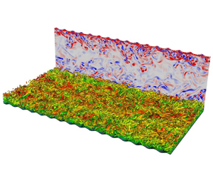
Figure 1(a) gives a schematic representation of the computational domain with figure 1(b) showing an enlarged view of the computational mesh. The top and bottom walls are symmetric around the midplane, i.e.  $y = \delta$. This enables averaging of the data across the top and bottom halves of the domain. Figure 1(a) also provides information about the various geometric parameters used to define the channel and surface roughness geometries. In general
 $x$,
 $y$ and
 $z$ are used to indicate streamwise, vertical (wall-normal for smooth wall) and spanwise directions with the corresponding velocity components being
 $u$,
 $v$ and
 $w$, respectively.
( $a$) Computational domain for turbulent channel flow simulation with sinusoidal walls at the top and bottom boundaries. (
 $b$) Enlarged view of the computational mesh in the
 $x$–
 $y$ plane showing the spectral elements for the
 $a^{+} = 18$,
 $\lambda = {\rm \pi}/8$ case. Each spectral element contains eight GLL points each in the
 $x$ and
 $y$ directions.

The fully developed turbulent channel flow is considered homogeneous in the streamwise and spanwise directions, enabling the use of periodic boundary conditions to increase the computational efficiency. No-slip wall boundary conditions are applied at the top and bottom walls. Identical domain sizes are used for all simulations in this study. All cases except case 4 use the exact same grid with the exception of the shape of the sinusoidal roughness. Case 4 uses a grid with more points in the streamwise direction to increase the number of points available to resolve each individual sinusoidal roughness element. The details of the grids are given in table 2.
Details of the computational grid for the DNS runs being presented in this study. The case numbers represent the corresponding runs from table 1. Here  $L_{i}$ indicates the mean domain extent in the
 $i$th coordinate direction, with
 $N_{el,i}$ and
 $N_{i}$ referring to the number of grid elements and the total number of grid points in the
 $i$th coordinate direction;
 $\Delta x_{min}$ and
 $\Delta x_{max}$ denote the minimum and maximum grid spacing in the streamwise (
 $x$) direction. The minimum and maximum grid spacings in the
 $y$ and
 $z$ directions are the same for all cases. The minimum and maximum grid spacings in inner units for the
 $y$ direction are
 $0.29$ and
 $1.9$, respectively. Similarly, for the
 $z$ direction the corresponding inner-scaled values are
 $2.27$ and
 $7.40$, respectively.

Although not long enough to capture the long wavelength outer-layer structures (Kim & Adrian Reference Kim and Adrian1999; Adrian, Meinhart & Tomkins Reference Adrian, Meinhart and Tomkins2000; Monty et al. Reference Monty, Stewart, Williams and Chong2007; Smits, McKeon & Marusic Reference Smits, McKeon and Marusic2011) the domain length in the streamwise direction is sufficient to correctly capture the near-wall low-frequency longitudinal streaks (Aubry et al. Reference Aubry, Holmes, Lumley and Stone1988) and preliminary simulations run for the smooth-wall mesh at  ${Re}_\tau =590$ matched the results of Moser, Kim & Mansour (Reference Moser, Kim and Mansour1999).
For the smooth-wall turbulent channel case, the simulation was conducted at a sub-Kolmogorov grid resolution with the Kolmogorov length scale,  $\eta =\nu ^{3/4}/\bar {\varepsilon }^{1/4}$, where
 $\bar {\varepsilon }$ is the temporally averaged dissipation rate of turbulent kinetic energy. The variation of the Kolmogorov scale relative to the grid spacing in the
 $y$ direction is given in figure 2. The smallest distance between two grid points, given by the Gauss–Legendre–Lobatto (GLL) quadrature, occurred at the wall with a value of
 $4.051 \times 10^{-4} \delta$ (
 $0.2899$ in inner units). Similarly, the largest distance between two GLL points in the grid occurred at the centreline and was
 $2.643 \times 10^{-3} \delta$ (
 $1.892$ in inner units).
Ratio of element averaged wall-normal grid-spacing,  $\Delta y$, to that of the element averaged Kolmogorov length scale,
 $\eta$.

Direct numerical simulations were performed for a total of six channel cases with one smooth-wall case and five wavy-wall cases where the amplitude,  $a$, and wavelength,
 $\lambda$, of the roughness was varied to generate different roughness profiles and examine the effect of these parameters on mean flow quantities and turbulence statistics. The vertical displacement of the sinusoidal surface at the bottom wall,
 $y_w$, relative to the surface of a smooth wall is given by
 \begin{equation} y_w(x)={-}a \sin \left(2 {\rm \pi}\tilde{x} \right), \end{equation}
where  $\tilde {x}=\text {mod}(x,\lambda )$. A summary of the geometric as well as flow parameters for all geometries which are a part of this study has been provided in table 1. To resolve each roughness element adequately, at least 32 points have been used to capture the individual elements in the streamwise direction. The short wavelength associated with the roughness element in case 4 made it necessary to employ a more resolved grid for this case. Care was taken to ensure that the maximum streamwise grid-spacing was always below 10 wall units, as shown in table 1.
The computational approach consisted of two main simulation stages. In the first stage, the flow was initialised using a laminar channel flow solution with some initial perturbations to accelerate the transition to turbulence. The skin friction values were monitored as a function of time to determine the statistical convergence of the fully turbulent flow. Once the flow was past the initial transient phase and had reached statistical convergence of the wall shear stress, a second stage was initiated in which in situ time-averaging of the flow field was performed to extract mean flow and turbulent statistics. These statistics were then monitored to ensure that statistical convergence was achieved for the entire flow field.
2.4. Averaging of flow data
The velocity components of the turbulent flow, e.g.  $u$, were decomposed into their time-averaged flow component
 $\bar {u}$ and a fluctuating part
 $u'$, so that
 \begin{equation} u = \bar{u} + u', \end{equation}
following Reynolds decomposition. Homogeneity in the  $x$ and
 $z$ directions for the smooth-wall case enabled spatial averaging of all flow quantities leading to one-dimensional distributions which only depend on the
 $y$ coordinate. For the sinusoidal rough-wall cases, the statistics remain homogeneous in the
 $z$ direction while becoming periodic in the
 $x$ direction with a wavelength of
 $\lambda$. Thus the two-dimensional flow field was averaged in the spanwise direction and averaged for each value of
 $y_w$ across a wavelength giving one-dimensional profiles varying with
 $\tilde {y}_w = y - y_w$. In general, an over-bar here indicates temporal averaging of a given quantity and
 $\langle \cdot \rangle$ indicates additional wavelength averaging that has been performed on the time-averaged quantities. The
 $\lambda$-periodicity of the wavy-wall cases also enables us to define
 $\tilde {x} = \text {mod}(x,\lambda )$, which acts as a non-dimensional distance ranging from
 $0$ to
 $1$.
One-dimensional profiles of wavelength-averaged quantities were obtained by averaging points at a constant vertical distance from the wall, specifically at constant  $\tilde {y} = y - y_w$. The non-dimensional sampling period,
 $T^{*} = Tu_\tau /\delta$ for each of the cases has been provided in table 1. Each of the cases have been spatially and temporally averaged for at least one flow through time,
 $T_f = L_x/U_b$.
3. Results
3.1. Instantaneous velocity fields
Figure 3(a–l) present example instantaneous fields of  $u/U_b$ and
 $v/U_b$ for each of the cases. As expected, increasing the amplitude of roughness corresponds to an increase in
 $u/U_b$ due to the increased confinement of the flow, however, otherwise there is little qualitative difference in
 $u/U_b$, as can be seen from figure 3(a,c,e,g,k). Compared with the smooth-wall case, there is a corresponding increase in the granularity of the
 $v$ component near the wall, as shown in figure 3(b,d,f,h,j,l), which is particularly noticeable with an increase in
 $a$. There also appears to be a qualitative increase in the scale of
 $v$ fluctuations near the centreline with increased
 $a$. However, quantitative investigation of such flow features by, for example, employing coherence analysis is beyond the scope of the present paper.
Colour contours of fully developed streamwise (a,c,e,g,i,k) and vertical (b,d,f,h,j,l) velocity fields for the six cases being analysed in this study. The colour bars at the top of (a,c,e,g,i,k) and (b,d,f,h,j,l) are for the streamwise and vertical velocity, respectively. (a) Smooth wall; (b) smooth wall; (c)  $a^{+} = 9$,
 $\lambda = {\rm \pi}/8$; (d)
 $a^{+} = 9$,
 $\lambda = {\rm \pi}/8$; (e)
 $a^{+} = 9$,
 $\lambda = {\rm \pi}/16$; (f)
 $a^{+} = 9$,
 $\lambda = {\rm \pi}/16$; (g)
 $a^{+} = 9$,
 $\lambda = {\rm \pi}/32$; (h)
 $a^{+} = 9$,
 $\lambda = {\rm \pi}/32$; (i)
 $a^{+} = 18$,
 $\lambda = {\rm \pi}/8$; (j)
 $a^{+} = 18$,
 $\lambda = {\rm \pi}/8$; (k)
 $a^{+} = 36$,
 $\lambda = {\rm \pi}/8$; (l)
 $a^{+} = 36$,
 $\lambda = {\rm \pi}/8$.

3.2. Mean velocity
The spatially averaged one-dimensional profiles of the mean streamwise velocity,  $\langle u \rangle ^{+}$, for all cases are shown in figure 4(a). There are noticeable effects of wavelength and amplitude on these profiles that are consistent with well-established effects of roughness on the mean streamwise velocity. In particular, the increase in the total drag force acting on the wall due to the pressure drag on the surface area normal to the flow results in a corresponding reduction in the magnitude of
 $\langle u \rangle ^{+}$ profiles; an effect represented by the roughness function defined in (1.2). Note that the Reynolds numbers considered in these simulations were not large enough to obtain a fully logarithmic overlap layer. However, there is an approximately logarithmic region evident in figure 4(a) initiating at a
 $\tilde {y}^{+}$ location that is dependent on the dimensions of the roughness elements. The slope of this approximately logarithmic region is also affected by the presence of the roughness. The change in the slope is most prominently seen for the green curve (
 $a^{+} = 36$,
 $\lambda = {\rm \pi}/8$ case) in figure 4(a).
Analysis of streamwise and wall-normal mean velocity components for all cases: ( $a$) spatially averaged one-dimensional profiles of the mean streamwise velocity,
 $\langle u \rangle ^{+}$; (
 $b$) modified scaling for
 $\langle u \rangle ^{+}$ following (1.2); (
 $c$) spatially averaged one-dimensional profiles of the mean velocity component in the
 $\tilde {y}$ direction,
 $\langle v \rangle ^{+}$; (
 $d$) effect of steepness on
 $\langle v \rangle ^{+}$. The vertical lines in (
 $b$) indicate the wall-normal locations corresponding to
 $(\tilde {y} - a)/\lambda = 0.3$ based on (
 $d$) after which the effect of the roughness is negligible and all profiles collapse. The filled-in square, triangle and diamond shapes on the
 $x$-axis in (
 $a$) and (
 $b$) show the location of the viscous scaled semiamplitude in the corresponding coordinate scale for
 $a^{+} = 9$,
 $a^{+} = 18$ and
 $a^{+} = 36$ cases, respectively.

The influence of the surface roughness on the scaling of the mean streamwise velocity is, therefore, well encapsulated by (1.1) with the roughness effect described by the parameters  $\Delta U^{+}$ and
 $y_0$, which manifest as the vertical shift in the approximately log layer and change of steepness of the mean velocity profile, respectively. For the present simulations, it was found that the roughness function values tabulated in table 3 provided the best agreement of the mean velocity profiles in the outer layer. It was also found that expressing
 $y_0 = y_0' + a_*$ provides the best results, where
 $y_0'$ is an amplitude-dependent length scale and
 $a_*$ is a constant which provides a shift in the virtual origin to account for the depth of the smooth-wall viscous sublayer which must be exceeded by
 $a$ for the flow to start exhibiting roughness effects. Using
 $y_0'=a/3$ and
 $a_*=5\nu /u_\tau$ brought the most consistent agreement amongst the profiles within the approximately logarithmic region. The roughness function was determined by finding the value of
 $\Delta U^{+}$ which provided the closest collapse of the data with the smooth-wall case once the virtual offset
 $y_0$ has been applied to the wall-normal coordinate.
Values of roughness parameters for each of the five roughness configurations.

This resulting agreement is shown in figure 4(b), which shows collapse of the scaled profiles for  $\tilde {y}^{+} -y_0^{+}\gtrapprox 100$. Below this point, the agreement of the rough-wall profiles with the smooth-wall profile becomes dependent on the geometry of the roughness.
A more contemporary approach to study the effect of surface roughness is to correlate the frontal solidity values for the roughness elements with the roughness function based on the density of roughness elements. Using the criterion that any roughness with  $\varLambda < 0.15$ belongs to the sparse regime and roughness with
 $\varLambda > 0.15$ belongs to the dense regime, cases 2, 3 and 5 correspond to the sparse regime, whereas cases 4 and 6 belong to the dense regime (see table 1). Jiménez (Reference Jiménez2004) and Flack & Schultz (Reference Flack and Schultz2014) have previously observed that the roughness function increases with the solidity in the sparse regime and decreases with the solidity in the dense regime. More recently, Placidi & Ganapathisubramani (Reference Placidi and Ganapathisubramani2015) and MacDonald et al. (Reference MacDonald, Chan, Chung, Hutchins and Ooi2016) reported that the distinction between the sparse and dense roughness regimes might not be at
 $\varLambda = 0.15$. While Placidi & Ganapathisubramani (Reference Placidi and Ganapathisubramani2015) observed that
 $\varLambda \geq 0.21$ marked the start of the dense regime, MacDonald et al. (Reference MacDonald, Chan, Chung, Hutchins and Ooi2016) noticed that
 $\varLambda \geq 0.18$ indicated the transition between these regimes. This distinction is even more uncertain when considering non-uniform surface roughness configurations (Napoli et al. Reference Napoli, Armenio and De Marchis2008), wherein the start of the dense regime can occur at
 $\varLambda$ values as high as
 $0.275$. The wide range of
 $\varLambda$ values which mark the beginning of the dense regime, would mean that any uniform roughness with
 $0.15 \leq \varLambda \leq 0.25$ can be in either of the two regimes. In their recent review paper, Chung et al. (Reference Chung, Hutchins, Schultz and Flack2021) mention that the transition to the dense regime (indicated by a peak in the drag), can lie in a very broad range, i.e.
 $0.1 \leq \varLambda \leq 0.3$.
While cases 2, 3 and 5 are most certainly in the sparse regime, cases 4 and 6 can be considered nominally dense, since the  $\varLambda$ values for these cases (
 $\varLambda = 0.2546$) are very close to the limiting values discussed above. The observed trends in
 $\Delta U^{+}$ for cases 2, 3 and 5 agree well with the previous literature (Jiménez Reference Jiménez2004; Napoli et al. Reference Napoli, Armenio and De Marchis2008; Flack & Schultz Reference Flack and Schultz2014; Placidi & Ganapathisubramani Reference Placidi and Ganapathisubramani2015; MacDonald et al. Reference MacDonald, Chan, Chung, Hutchins and Ooi2016; Chung et al. Reference Chung, Hutchins, Schultz and Flack2021) showing an increase in
 $\Delta U^{+}$ with increasing
 $\varLambda$. For roughness in the dense regime, the roughness function is expected to decrease with increasing
 $\varLambda$, but this trend is not observed for cases 4 and 6. The roughness function still increases despite the frontal solidity being above the conventional threshold value of
 $\varLambda = 0.15$. It should be noted that this is a relatively small sample size that was used, and it would be very difficult to generalise these trends based on only five cases. However, keeping in view with conventional estimates, cases 4 and 6 will be referred to as being nominally dense hereafter.
Another important observation is that despite having the same  $\varLambda$ the values of
 $\Delta U^{+}$ are vastly different for cases 3 and 5, and cases 4 and 6, indicating that
 $\varLambda$ alone is not sufficient to completely capture the effects of surface roughness. The present study provides an analysis of a limited set of roughness element configurations due to the extremely high computational costs associated with these simulations, however, these results reinforce what has previously been observed in the literature. It is extremely difficult to quantify the effects of surface roughness on turbulent flows without considering a combined effect of the geometrical parameters of the roughness. Cases 2, 3, 4 and 5 have shown that regardless of the roughness regime, roughness configurations having the same
 $\varLambda$ (or
 $\sigma$) values can have different roughness functions and drag values.
Although the value of  $y_0$ appears to be a function of
 $a$, the increase in
 $\Delta U^{+}$ was related to both decreasing
 $\lambda$ and increasing
 $a$. We can also examine
 $k_s$, commonly described as a fraction of
 $a$ (hence a function of only
 $a$). To find
 $k_s$, we first note that the values of
 $\Delta U^{+}$ reflect that the flow was transitionally rough for the majority of the cases examined. Therefore, the
 $k_s$ and
 $k_s^{+}$ values for the various rough-wall cases were estimated using Colebrook's interpolation formula (Colebrook Reference Colebrook1939)
 \begin{equation} \Delta U^{+} = \kappa^{{-}1}\ln(1+0.26 k_s^{+}), \end{equation}
and the corresponding values are included in table 3. It should, however, be pointed out that case 6 is in the nominally dense regime, and using Colebrook's interpolation formula might not be the best way to obtain  $k_s^{+}$. For fully rough flows, (1.2) is used to estimate
 $k_s^{+}$ by substituting
 $k_s^{+}$ for
 $k^{+}$. Using (1.2) for case 6 with
 $\kappa = 0.40$ and
 $B = 5.3$, we obtain
 $k_s^{+} = 134.83$, which is within 5 % of the value obtained using (3.1), further providing evidence that this case lies at the edge of the transitionally rough and fully rough regimes and can be considered nominally rough. As expected,
 $k_s$ is dependent on both
 $a$ and
 $\lambda$, and not just on the steepness,
 $\sigma$. Specifically, the same values of either
 $a$,
 $\lambda$ or
 $\sigma$ can produce different values of
 $k_s$ depending on the values of the other topographical parameters. This then defines the scaling problem addressed in the remainder of the paper. Namely, identifying which roughness effects can be attributed to which geometrical parameter.
One effect the surface roughness will have is the introduction of a non-zero wall-normal mean velocity,  $\langle v \rangle$. The
 $\langle v \rangle ^{+}$ profiles are presented in figure 4(c). The presence of a non-zero
 $\langle v \rangle$ constitutes a deviation from the smooth-wall case and, therefore, reflects the influence of surface roughness and can be used to define the extent of the roughness sublayer. Notably, figure 4(c) illustrates that the wall-normal location at which
 $\langle v \rangle$ becomes zero does not appear to correlate with an increase in drag (and
 $\Delta U^{+}$).
To examine the geometric dependence of the location of vanishing  $\langle v \rangle$, figure 4(d) shows the dependence of the profiles of
 $\langle v \rangle ^{+}$ on
 $\lambda$ relative to the distance above the peak of the roughness,
 $(\tilde {y}-a)/\lambda$. These coordinates reflect the role of steepness in production of the roughness sublayer as it becomes apparent that, for all cases, the influence of roughness is largely confined to
 $0.3\lambda$ above the peak of the roughness amplitude with the greatest deviation from the smooth-walled case occurring for
 $(\tilde {y}-a) \lessapprox 0.1 \lambda$. It therefore appears that the extent of the roughness sublayer depends on
 $\lambda$, rather than
 $a$, as one would intuitively expect. MacDonald et al. (Reference MacDonald, Ooi, García-Mayoral, Hutchins and Chung2018) showed a clear dependence of the roughness function on the wavelength of the roughness element, albeit for very dense two-dimensional roughness geometries (
 $0.25 < \varLambda < 3.0$). This dependence of the roughness function on not just the roughness amplitude and steepness (solidity) but also on the roughness wavelength for sparse and dense regimes makes it very important to consider the role of roughness wavelength in determining the appropriate length scales for roughness affected turbulent flows. The effect of the roughness wavelength on the flow structures is explored in greater detail in the following sections. To further illustrate this point, the location corresponding to
 $(\tilde {y}-a)=0.3\lambda$ indicated by vertical lines are shown in figure 4(b), and can be seen to closely correspond to the location where each roughness case begins to approximately deviate from the smooth-walled case.
3.3. Mean vorticity within the roughness
To assess the region of influence for the roughness elements in more detail, figure 5 presents streamtraces of the two-dimensional mean velocity overlaid on contours of the time-averaged spanwise normalised vorticity
 \begin{equation} \left\langle\omega\right\rangle=\frac{\partial \left\langle v\right\rangle}{\partial x}-\frac{\partial \left\langle u\right\rangle}{\partial y} , \end{equation}
presented as isocontours of  $\langle \omega \rangle \lambda /u_\tau$. The flow field around a large-amplitude wavy surface has previously been observed to consist of three regions (Buckles, Hanratty & Adrian Reference Buckles, Hanratty and Adrian1984; Hudson et al. Reference Hudson, Dykhno and Hanratty1996) which were evident in all cases shown in figure 5: (1) a pocket of recirculating flow in the wake of the crest; (2) a boundary layer over the crest; and (3) a shear layer separating from the recirculation region from the flow above the cavity. The shear layer extending across the cavity thickens in the downstream direction and impinges onto the windward portion of the roughness element. With increasing steepness, the shear layer thickens relative to the wavelength and spanwise vorticity near the crest increases in intensity.
Contours of normalised mean vorticity,  $\langle \omega \rangle \lambda / u_\tau$ superimposed with streamtraces of the velocity field for: (a)
 $a^{+}=9$,
 $\lambda ={\rm \pi} /8$; (b)
 $a^{+}=9$,
 $\lambda ={\rm \pi} /16$; (c)
 $a^{+}=9$,
 $\lambda ={\rm \pi} /32$; (d)
 $a^{+}=18$,
 $\lambda ={\rm \pi} /8$; and (e)
 $a^{+}=36$,
 $\lambda ={\rm \pi} /8$. Negative contour levels are indicated by dashed contour lines and the location of
 $y_0^{\prime\prime}$ for each case is indicated by a dashed blue line. The white line near the roughness trough indicates the contour of zero-vorticity.

A corresponding increase in the size of the recirculation regions can also be observed in the streamline visualisations in figure 5 reflecting the transition from  $k$-type to
 $d$-type roughness with both increasing
 $a$ and decreasing
 $\lambda$, i.e. correlated to the increase in steepness of the elements. The demarcation between
 $k$- and
 $d$-type roughness regimes is not very well defined; however, it has been linked to the relative contributions of the pressure drag and the skin drag to the total drag acting on the wall in a study by Leonardi, Orlandi & Antonia (Reference Leonardi, Orlandi and Antonia2007). Figure 6 provides the roughness function for flows in the fully rough regime over a range of roughness geometries obtained using DNS by Leonardi et al. (Reference Leonardi, Orlandi and Antonia2007). The filled-in red squares indicate a
 $d$-type roughness since the roughness function is independent of the roughness height. Although the cases being considered in the present study are not in the fully rough regime, the dependence of roughness function on amplitude (and steepness) indicates the presence of a
 $k$-type roughness.
The variation of roughness function for different roughness geometries using different roughness height to width ratios for flows in the fully rough regime plotted against the inner-scaled roughness height (or amplitude). The filled-in data points have been adapted from Leonardi et al. (Reference Leonardi, Orlandi and Antonia2007) with the solid straight lines following (1.2). The roughness function for the cases considered in the current study have been plotted as individual symbols. The square, triangle and circle symbols indicate cases with the same roughness amplitude ( $a^{+} =9$) and wavelengths corresponding to
 $\lambda ={\rm \pi} /8$,
 $\lambda ={\rm \pi} /16$ and
 $\lambda ={\rm \pi} /32$, respectively. Similarly, the plus and asterisk symbols are used to indicate cases at a constant wavelength (
 $\lambda = {\rm \pi}/8$) with amplitude
 $a^{+} = 18$ and
 $a^{+} = 36$, respectively.

Flow separation can be identified for all wavelengths and wave amplitudes. At lower steepness, the streamlines are diverted lower into the cavity with a corresponding lower reattachment point of the recirculation region. As steepness increases, the reattachment point moves closer to the peak in the surface. These results are consistent with the general observation that the flow inside the recirculation regions with larger steepness appears to be more isolated from the flow above the cavities. The effects of the two-dimensional roughness diminish by  $(y-a)\sim 0.3\lambda$ (see figure 5) which is consistent with the observations for the mean
 $\langle v \rangle ^{+}$ in figure 4(d). Now,
 $y_0'$ is defined in the context of
 $\tilde {y}$ which represents a fixed distance
 $a/3$ units above the wall in the terrain-following coordinates given by
 $\tilde {y}$. However, in two dimensions, using a similar procedure to define the roughness offset is not straightforward. Instead, we used the location at which the mean spanwise vorticity
 $\omega$ switches sign to define the roughness offset. Coincidentally, this location was found to occur approximately
 $a/3$ units above the trough of the roughness element. This distance will henceforth be denoted as
 $y_0'' = -2a/3$. The location of
 $y_0''$ is marked in all plots of figure 5 with corresponding dashed horizontal lines and it is found to roughly correspond to the lowest location at which the vorticity is negative, or the lowest extent of the vorticity layer as shown by the solid white line in figure 5. Although the depth of the roughness sublayer in the mean flow scales with
 $\lambda$, within the roughness sublayer, the statistics and shear stress display a dependence on both
 $a$ and
 $\lambda$ which has been attributed to the predominance of the shear layer within the roughness elements (Hudson et al. Reference Hudson, Dykhno and Hanratty1996). We thus introduce a shear velocity scale,
 $U_{sl}$, and shear length scale,
 $\ell _{sl}$, intended to describe the strength and thickness of the separated shear layer within the roughness elements.
To approximate  $U_{sl}$, we use the value of
 $\langle u \rangle$ of the undisturbed (i.e. smooth-wall) flow at a distance from the wall corresponding to trough-to-peak amplitude of the roughness element. We also compensate for the roughness offset,
 $y_0'$ or
 $y_0''$ in two dimensions. Thus,
 $U_{sl}$ is defined as the value of
 $\langle u \rangle$ from the smooth-wall case at
 $y^{+} = 5a^{+}/3$. It should be noted that as
 $a \rightarrow 0$,
 $U_{sl}$ also approaches
 $0$. This inherently adds limitations on using
 $U_{sl}$ for normalising physical quantities such as vorticity or other higher-order turbulent statistics. Therefore, its suitability as a scaling parameter is unlikely for roughness geometries lying well within the viscous sublayer, i.e.
 $a^{+} \ll 5$.
To approximate  $\ell _{sl}$, which we expect to be related to a mixture of both
 $a$ and
 $\lambda$ and influences the spreading rate of the shear layer, we use the form
 $\ell _{sl}=a^{\beta } \lambda ^{1-\beta }$, where
 $\beta$ is an empirically determined parameter. This expression can also be written as
 $\ell _{sl} = \sigma ^{\beta } \lambda$, where the spreading rate of the shear layer is purely a function of the steepness,
 $\sigma$, and wavelength,
 $\lambda$. The magnitude of the shear-layer vorticity was found to be much more uniform and similar across all cases when
 $\beta = 0.6$. Hereafter, we use the subscript
 ${sl}$ to indicate a parameter normalised by these shear-layer parameters.
Figure 7 shows the wavelength-averaged  $\langle \omega \rangle _{sl} = \langle \omega \rangle \ell _{sl}/U_{sl}$ field. Also,
 $y_{sl} = y/\ell _{sl}$ is the non-dimensional value of
 $y$ obtained using the corresponding shear-layer variable. The results show that the magnitude of the vorticity within the shear layer (marked by the region shown in green) is approximately constant. Notably, the boundary layers forming just downstream of the shear-layer impingement location do not scale with these length and velocity scales.
Contours of  $\langle \omega \rangle _{sl}$ superimposed with streamtraces of the velocity field for: (a)
 $a^{+}=9$,
 $\lambda ={\rm \pi} /8$; (b)
 $a^{+}=9$,
 $\lambda ={\rm \pi} /16$; (c)
 $a^{+}=9$,
 $\lambda ={\rm \pi} /32$; (d)
 $a^{+}=18$,
 $\lambda ={\rm \pi} /8$; and (e)
 $a^{+}=36$,
 $\lambda ={\rm \pi} /8$.

The validity of this scaling is further examined in the one-dimensional profiles of  $\langle \omega \rangle _{sl}$ shown in figure 8(a). Two distinct regions are observed and are marked as regions
 $I$ and
 $II$ in figure 8(a). Region
 $I$ corresponds to the layer below the roughness offset that is influenced by the viscous shear stress at the peak of the roughness elements, and reversed flow within the trough of the roughness elements. This region is responsible for the generation of skin friction and is linked to the high gradients occurring at the wall. To better understand the behaviour of peak vorticity (which occurs at the wall), we extract the peak values for each of the sinusoidal wall cases,
 $|\langle \omega \rangle _{sl}|_{wall}$, and examine its dependence on the geometrical parameters of the roughness. We found that instead of having a dependence on amplitude or wavelength alone, the magnitude of peak vorticity scales with the steepness of the roughness element and is given by
 \begin{equation} |\langle \omega \rangle _{sl}|_{wall} = 0.336 \left(\frac{2a}{\lambda} \right)^{{-}0.75}. \end{equation}
A comparison of the shear-scaled vorticity at the wall obtained using DNS and using (3.3) is shown in figure 8(b). Region  $II$ corresponds to the layer where the shear layer influences the statistics. Specifically, there is the emergence of a secondary peak in
 $\langle \omega \rangle _{sl}$ at
 $(\tilde {y} - y_0' -a_*)/a \approx 0.55$, corresponding to the impingement of the shear layer on the roughness element. This peak becomes increasingly evident with increasing
 $\Delta U^{+}$, i.e. as the roughness transitions towards the fully rough condition. Moving farther away from the roughness element, the effects of the roughness on the flow diminish and the vorticity drops to zero similar to flow over a smooth wall as observed in region
 $III$.
(a) Shear-scaled profiles of vorticity,  $\langle \omega \rangle _{sl}$. The dashed vertical lines (red) divide the plot into three different regions and the vertical dash–dotted line (pink) shows the approximate location of the secondary peak in vorticity due to the presence of the shear layer. The colours and patterns for the profiles are the same as given by the legend in figure 4. (b) Comparisons between the steepness-based model and DNS for the shear-scaled vorticity at the wall. The symbols used to indicate the different cases remain unchanged from figure 6 with the straight line indicating a perfect match.

3.4. Pressure distribution within the roughness
Noting that for most cases (cases 3–6) the increase in  $\Delta U^{+}$ due to roughness is primarily caused by pressure drag on the roughness elements (see table 3), we now examine the changes in the pressure field within the roughness elements. We begin with modelling the increase in pressure due to stagnation on the roughness element as
 $P_{stag}= \rho U_{stag}^{2} / 2$, where
 $U_{stag}$ is the velocity of the stagnation streamline and is derived using the shear-layer velocity introduced in § 3.3.
The stagnation velocity was obtained by assuming the diffusion of  $U_{sl}$ along the length of the shear layer. This diffusion was found to be poorly modelled by either a diffusing wake or a free shear layer, prohibiting the use of either geometry's established similarity models to predict the diffusion characteristics. We instead begin with a generalised model for the stagnation velocity given by
 \begin{equation} U_{stag} = U_{sl} - \delta U, \end{equation}
where  $\delta U$ is the reduction in shear-layer strength due to diffusion of the shear layer. Hence, the introduction of
 $\delta U$ captures the
 $\lambda$-dependent effects of the shear-layer diffusion arising from the streamwise diffusion shear layer, whereas the
 $a$-dependent effects are contained within
 $U_{sl}$.
Since the diffusion of the shear layer does not follow any standard similarity-based diffusion model, we introduce an exponent,  $m$ to account for the diffusing wake based on the wavelength. This leads to an expression for the velocity deficit of the form
 \begin{equation} \delta U = c U_{sl} \left( \frac{\lambda}{\delta} \right)^{m}. \end{equation}
We found that the values of  $0.47$ and
 $-0.085$ for
 $c$ and
 $m$, respectively, provided the best agreement with the DNS results for stagnation pressure, as shown in figure 9. This model for the stagnation pressure was able to predict the stagnation pressure for all cases with a root mean square error of less than 3 %.
Comparisons between the stagnation pressure value obtained from DNS and the proposed model. The symbols used to indicate the different cases remain unchanged from figure 6 with the straight line indicating a perfect match.

Isocontours of the wavelength-averaged pressure field are shown in figure 10. It was found that the pressure field within the roughness elements did not scale well with  $u_\tau$. Instead, noting the importance of the shear layer on the pressure field and the stagnation pressure, the pressure fields for the sinusoidal wall cases in figure 10 are presented as a pressure coefficient based on
 $U_{stag}$,
 \begin{equation} C_{P_{stag}}=\frac{\langle P \rangle}{\frac 12 \rho U_{stag}^{2}}. \end{equation}
Contours of pressure coefficient,  $C_{P_{stag}}$, overlaid by the streamtraces of the velocity field for the: (a)
 $a^{+}=9$,
 $\lambda ={\rm \pi} /8$; (b)
 $a^{+}=9$,
 $\lambda ={\rm \pi} /16$; (c)
 $a^{+}=9$,
 $\lambda ={\rm \pi} /32$; (d)
 $a^{+}=18$,
 $\lambda ={\rm \pi} /8$; and (e)
 $a^{+}=36$,
 $\lambda ={\rm \pi} /8$ cases.

One-dimensional profiles of: (a) inner-scaled turbulent kinetic energy,  $K^{+}$; (b)
 $\langle u'u' \rangle ^{+}$; (c)
 $\langle v'v' \rangle ^{+}$; (d)
 $\langle w'w' \rangle ^{+}$; (e)
 $\langle u'v' \rangle ^{+}$; and (f) turbulent kinetic energy in shear scaling. The vertical dash–dotted line (pink) in (
 $f$) shows the approximate location of the maxima for the shear-scaled
 $K$. The colours and patterns for the profiles are the same as given by the legend in figure 4 with the vertical lines showing the location at which the
 $v$ component of velocity collapses in figure 4(d). The filled-in square, triangle and diamond shapes on the
 $x$-axis show the location of the viscous scaled semiamplitude in the corresponding coordinate scale for
 $a^{+} = 9$,
 $a^{+} = 18$ and
 $a^{+} = 36$ cases, respectively.

The pressure fields shown in figure 10 consistently display two strong positive and negative regions of pressure, both scaling well with  $\rho U_{stag}^{2}/2$. The positive pressure region corresponds to the stagnation point where the separated shear-layer impinges on the windward face, and will have the strongest contribution to pressure drag. The location of this stagnation point depends on the steepness of the roughness elements, moving closer to the crest of the elements with increasing steepness.
A region of low pressure of equivalent magnitude occurs just downstream of the crest and is attributed to the acceleration of the flow immediately following the impingement location on the windward side of the roughness element. Since the low pressure region only acts over a small portion near the crest of the surface roughness, its contribution to pressure drag will be much smaller than the positive pressure region on the windward face of the roughness element. For the high steepness cases, there is an additional negative pressure region that forms within the roughness trough due to the stronger recirculation for these cases.
Table 3 provides the resulting relative contributions of skin friction and pressure (form) drag to the total drag for the rough-wall cases. Comparing the ( $a=0.0125$,
 $\lambda ={\rm \pi} /32$) and (
 $a=0.025$,
 $\lambda ={\rm \pi} /8$) cases, it can be seen that although
 $\Delta U^{+}$ increases between the two cases, both
 $k_s/a$ and proportion of pressure drag decreases, reflecting the dependence of
 $k_s/a$ on details of the roughness sublayer. Similarly, as evident from figure 10, the magnitude of
 $C_{P_{stag}}$ at the stagnation point is similar for all cases. However, there is still some dependence on the steepness of the roughness, as this affects the impingement point and diffusion of the shear layer when it separates from the upstream element crest and impinges on the downstream element face. These will be revisited in § 4 to develop a model for the pressure (form) and viscous (skin) drag components.
3.5. Turbulent kinetic energy and Reynolds stresses
We now move on to a discussion of second-order turbulent statistics, i.e. turbulent kinetic energy and the Reynolds stresses. While we were able to identify rough scaling laws for the mean flow profiles, scaling turbulent statistics will be more challenging. Profiles of mean turbulent kinetic energy,  $K = ( \langle u'u' \rangle + \langle v'v' \rangle + \langle w'w' \rangle )/2$ are presented in figure 11(a) using inner scaling. A collapse of profiles in the outer region consistent with Townsend's outer-layer similarity hypothesis was observed for the inner-scaled turbulence statistics as shown in figure 11(a–e) (recall that since all cases are at equivalent
 ${Re}_\tau$, the same
 $\tilde {y}^{+}$ location for each case will also correspond to the same
 $\tilde {y}/\delta$ location). Hence, as was observed with the mean velocity profiles, the effects of differing roughness geometries are confined to the near-wall region of the flow, with this region of influence depending on both the amplitude and wavelength of the surface roughness. Unlike the mean-flow statistics for which the roughness sublayer appeared to scale with
 $\lambda$, for the turbulence statistics the depth of this region of influence was found to be affected more by
 $a$, which can be attributed to the shear layer being displaced away from the surface with increasing
 $a$.
Also evident in figure 11(a) is the variability in the location of the near-wall peak in  $K$. For the smooth-wall case this peak corresponds to the near-wall production cycle and occurs at a
 $y^{+} \approx 12$. For the wavy-wall cases, this peak can be attributed to turbulence production within the shear layer and its reduced prominence at larger
 $a$ also reflects a decreased contribution to
 $K$ coming from the
 $\langle u'u' \rangle$ normal Reynolds stress, shown to decrease with increasing
 $a$ in figure 11(b). A direct consequence of these changes in the distribution of Reynolds stresses is an increasing separation of the inner (close to the surface roughness) and outer (towards the centre of the channel) flow regions as is also observed in the streamwise velocity flow visualisations from figure 3.
Despite significant deviations of the components of the Reynolds stress tensor, i.e.  $\langle u'u' \rangle$,
 $\langle v'v' \rangle$,
 $\langle w'w' \rangle$ and
 $\langle u'v' \rangle$ from the smooth wall cases in the near wall regions, the profiles of
 $\langle v'v' \rangle$,
 $\langle w'w' \rangle$ and
 $\langle u'v' \rangle$ remain largely unaffected, as shown in figure 11(c,d). The peak magnitude and locations for these quantities were almost unchanged across all cases unlike for
 $\langle u'u' \rangle$, which has a much more prominent effect of the roughness showing a clear
 $a$-dependent peak location reflecting its dependence on the shear-layer location.
The effect of the shear layer is also apparent in the profiles of  $\langle u'v' \rangle ^{+}$ shown in figure 11(e). This effect is especially prominent in the cases with different amplitudes, where a secondary peak is developing below the region where the rough-wall cases collapse with the smooth-wall case.
The  $a$-dependence of the Reynolds stresses is summarised in figure 11(f), which displays the
 $a$-dependence of the peak in
 $K$, which for all rough-wall cases was found to occur close to
 $(\tilde {y} - y_0' - a_*)/a = 1.6$, which we attribute to the displacement of the shear layer due to the roughness height. However, the magnitude of the peak values of
 $K_{sl}$ demonstrate dependence on
 $a$ and
 $\lambda$, suggesting that the shear layer alone is not responsible for the distribution of
 $K$ near the wall. Further insight into the effects of the roughness on the characteristics of turbulent flow can be obtained by examining the turbulent kinetic energy transport budget
 \begin{align} \underbrace{\frac{\partial K}{\partial t}}_{\substack{\text{Rate of change} \\ \text{of }K}} &= \underbrace{-\left\langle u_i^{'} u_j^{'}\right\rangle \frac{\partial \left\langle{u_i}\right\rangle}{\partial x_j}}_{\text{Production}} - \underbrace{\left\langle\varepsilon\right\rangle}_{\substack{\text{Turbulent} \\ \text{dissipation}}}\nonumber\\ &\quad - \underbrace{\frac{\partial}{\partial x_j} \left\{\underbrace{\left\langle K\right\rangle \left\langle{u_j}\right\rangle}_{\substack{\text{Convection} \\ \text{by meanflow}}} + \underbrace{\left\langle u_j^{'} \left(K+\frac{p}{\rho}\right)\right\rangle - \nu \left\langle u_i^{'} \left(\frac{\partial u_i^{'}}{\partial x_j} + \frac{\partial u_j^{'}}{\partial x_i}\right)\right\rangle}_{\text{Diffusion}}\right\}}_{\text{Transfer of turbulent energy}}, \end{align}
where we have used index notation for compactness such that ( $u_1,u_2,u_3$) corresponds to the Cartesian velocity components (
 $u,v,w$), and likewise (
 $x_1,x_2,x_3$) corresponds to the (
 $x,y,z$) directions, respectively. Each of the terms in (3.7) represents a mechanism by which
 $K$ can either be locally produced, dissipated and/or redistributed. In the stationary turbulent flow considered here, the time rate of change of
 $K$ is identically zero and the flow can be considered homogeneous in the
 $z$ direction so that the time-averaged quantities are independent of the
 $z$ direction.
All terms from (3.7) are presented as one dimensional profiles in figure 12, normalised using shear-layer scaling, i.e. normalised by  $U_{sl}^{3}/\ell _{sl}$. The profiles of shear-scaled production,
 $P_{sl}$, shown in figure 12(a) are found to scale extremely well with the shear-layer scaling and collapse onto each other with peak production occurring at
 $(\tilde {y} - y_0' - a_*)/a \approx 1.25$. This location closely corresponds to the peak location of the shear-scaled
 $K$ in figure 11(f). The similar locations for the peak
 $K_{sl}$ and peak
 $P_{sl}$ provides support to the strong influence of the shear-layer dynamics on the characteristics of turbulent flows affected by surface roughness. Consequently, using shear-layer scaling provides a mechanism which was used to characterise the behaviour of
 $K$. More importantly, this characterisation was based solely on the geometric parameters of the roughness and the mean velocity profile from the smooth wall case at the given
 ${Re}_\tau$.
One-dimensional profiles of shear-layer-scaled terms from the turbulent kinetic energy transport equation: (a) production,  $P_{sl}$; (b) dissipation,
 $\langle \varepsilon \rangle _{sl}$; (c) convection by mean flow,
 $MC_{sl}$; (d) turbulent diffusion,
 $TD_{sl}$; (e) pressure diffusion,
 $PD_{sl}$; and (f) viscous diffusion,
 $VD_{sl}$. The dash–dotted line (pink) shows the approximate location of peak turbulence production in each of the plots. The colours and patterns for the profiles are the same as given by the legend in figure 4 with the vertical lines showing the location at which the
 $v$ component of velocity collapses in figure 4(d). The filled-in square, triangle and diamond shapes on the
 $x$-axis show the location of the viscous scaled semiamplitude in the corresponding coordinate scale for
 $a^{+} = 9$,
 $a^{+} = 18$ and
 $a^{+} = 36$ cases, respectively.

Interestingly, similar behaviour is observed for  $\langle \varepsilon \rangle _{sl}$. As with the profiles of
 $\langle \omega \rangle _{sl}$ shown in figure 8(a), there is increased influence of the boundary layer region for small
 $\tilde {y}$. Although the profiles of turbulent diffusion,
 $TD_{sl}$, pressure diffusion,
 $PD_{sl}$ and viscous diffusion
 $VD_{sl}$ do not show the same level of agreement as those of
 $P_{sl}$ and
 $\langle \varepsilon \rangle _{sl}$, local minima in these values correspond to the location at which the peak occurs for
 $P_{sl}$ (figures 12d–f). Conversely, the distributions of convection by the mean flow,
 $MC_{sl}$, do not appear to show the same alignment with the shear layer, as shown in figure 12(c).
Despite considering a much higher Reynolds number here when compared with previous experimental (Hudson et al. Reference Hudson, Dykhno and Hanratty1996) and computational studies (De Angelis et al. Reference De Angelis, Lombardi and Banerjee1997), the general trends for the production and dissipation terms remain largely unchanged with peak production occurring close to the separation point in the vicinity of the wall. Further insight into the mechanisms responsible for the production of  $K$ can be obtained by considering the constituent terms of the production
 \begin{equation} P ={-}\left\langle u_i^{'} u_j^{'}\right\rangle \frac{\partial \left\langle{u_i}\right\rangle}{\partial x_j} ={-}\left( \underbrace{\langle u'u' \rangle \frac{\partial \langle u \rangle}{\partial x}}_{P_{11}} + \underbrace{\langle u'v' \rangle \frac{\partial \langle u \rangle}{\partial y}}_{P_{12}} + \underbrace{\langle u'v' \rangle \frac{\partial \langle v \rangle}{\partial x}}_{P_{21}} + \underbrace{\langle v'v' \rangle \frac{\partial \langle v \rangle}{\partial y}}_{P_{22}} \right). \end{equation}
For the rough-walled cases, additional mean velocity gradients are introduced relative to the smooth-wall case, along with a corresponding deviation in the Reynolds stress distributions. Notably, these distributions are heavily dependent on the dynamics of the shear layer near the surface roughness. We can obtain some additional insight into the flow physics around the roughness by looking at the individual terms from (3.8). The contribution of the individual terms from (3.8), i.e.  $P_{11}$,
 $P_{12}$,
 $P_{21}$ and
 $P_{22}$, are displayed in figure 13(a–d), for the
 $a^{+} = 9$,
 $\lambda = {\rm \pi}/8$ case. As expected, the major contribution to turbulence production can be attributed to
 $P_{12}$ and is localised in the shear layer. Now
 $P_{11}$ has a slightly smaller contribution, largely concentrated in the boundary layer due to the significantly large value of
 $\langle u'u' \rangle$ coupled with a non-diminishing mean velocity gradient in the streamwise direction introduced by the roughness. It was found that the combined contribution of
 $P_{11}$ and
 $P_{12}$ was more than an order of magnitude larger than that of
 $P_{21}$ and
 $P_{22}$, as can also be observed from figure 13. Furthermore, the contributions from the
 $P_{11}$ and
 $P_{12}$ terms were found to mostly show opposite signs throughout the domain, effectively cancelling each other. The trends observed for the constituent terms of
 $K$ production are consistent with what has been previously observed experimentally by Hudson et al. (Reference Hudson, Dykhno and Hanratty1996).
Contour plots of the constituent terms of  $K$ production in shear scaling, for: (a)
 $P_{11}$; (b)
 $P_{12}$; (c)
 $P_{21}$; and (d)
 $P_{22}$ for the
 $y^{+} = 9$,
 $\lambda = {\rm \pi}/8$ case. The colour bar on the top applies for (a,b) whereas the colour bar at the bottom is used for (c,d).

As the production and dissipation of turbulence are going to be dominated by the impingement of the shear layer separating from the roughness elements, it is not unexpected that the magnitude of these quantities will scale with  $U_{sl}$ and
 $\ell _{sl}$, with the peak location following the trajectory of the shear layer, which will itself depend on
 $a$. However, as shown in figure 14, the distributions of the combined diffusion terms are more complex. Generally, the same structure is present near the shear layer. This structure has two major regions where
 $K$ diffusion is present. The two regions from which diffusion occurs have been marked using arrows in figure 14(a). In the first region turbulence is diffusing away from the high
 $K$ region around the shear layer into the trough of the roughness, and in the second region
 $K$ diffuses towards the impingement point from the shear layer. These regions are formed by the high
 $K$ diffusing away from its peak in the shear layer, as shown by the contour lines of
 $K$ in figure 14(a–e).
Distributions of  $TD_{sl}+PD_{sl}+VD_{sl}$ for: (a)
 $a^{+}=9$,
 $\lambda ={\rm \pi} /8$; (b)
 $a^{+}=9$,
 $\lambda ={\rm \pi} /16$; (c)
 $a^{+}=9$,
 $\lambda ={\rm \pi} /32$; (d)
 $a^{+}=18$,
 $\lambda ={\rm \pi} /8$; and (e)
 $a^{+}=36$,
 $\lambda ={\rm \pi} /8$. The labelled contour lines correspond to the levels of the turbulent kinetic energy.

Noticeable, however, is also the presence of an additional layer above the shear layer, with the distance of these regions away from the surface no longer scaling with  $a$. For the low steepness case, figure 14(a), regions of positive and negative diffusion extend to
 $(y + y_0'' - a_*)/a \approx 5$, whereas the high steepness cases of figure 14(d–e) show evidence of these same structures at
 $(y + y_0'' - a_*)/a \approx 3$. Furthermore, the secondary layer can be seen to be occurring much farther away from the surface roughness for the cases with smaller wavelengths, i.e. figure 14(b,c). This behaviour reflects the influence of advection from upstream roughness elements and hence introduces a dependence on
 $\lambda$, thereby providing rationale for why the depth of the roughness sublayer displays dependence on
 $\lambda$ as shown in the contour plots for vorticity in figure 5.
Similar to the diffusion terms,  $\lambda$-dependence can also be observed in the
 $MC_{sl}$ distributions shown in figure 15 and further reflecting the advection of turbulence produced by upstream roughness elements. We also see that the role of the shear layer is quite small for the low steepness case of figure 15(a), indicating that the mean advection for this case is dominated by the advection from upstream elements. Conversely, for the high steepness case of figure 15(e), the shear layer displays increased importance in the mean advection.
Distributions of  $MC_{sl}$ for: (a)
 $a^{+}=9$,
 $\lambda ={\rm \pi} /8$; (b)
 $a^{+}=9$,
 $\lambda ={\rm \pi} /16$; (c)
 $a^{+}=9$,
 $\lambda ={\rm \pi} /32$; (d)
 $a^{+}=18$,
 $\lambda ={\rm \pi} /8$; and (e)
 $a^{+}=36$,
 $\lambda ={\rm \pi} /8$.

The mixed role of  $a$ and
 $\lambda$ in scaling the extent and behaviour within the roughness sublayer thus reflects the conflicting importance of local shear-layer dynamics and non-local diffusion and advection from upstream elements. In addition, the dependence of advected and diffused
 $K$ illustrates why the profiles of
 $K$ in figure 11(e) do not scale with shear-layer properties alone. Although not a particularly surprising observation, these results provide clear evidence of the relative dependence of this behaviour, and suggests that even in very simple roughness, one cannot neglect the role of
 $\lambda$ in the scaling of the roughness behaviour.
4. Characterisation of drag
4.1. Pressure drag
The previous sections illustrated how the shear layer is the predominant feature within the roughness elements, and establishes that  $U_{sl}$ characterises the strength of the shear layer. Here, we use this information to develop a semiempirical model to predict the drag on the sinusoidal roughness elements, i.e. the effective wall shear stress.
We first recognise that the pressure drag is almost entirely driven by the stagnation pressure on the windward face of the roughness element. Hence, to predict the pressure drag, we require estimates of the location of the stagnation point, the stagnation pressure,  $P_{stag}$, and the distribution of pressure around the stagnation point.
The reconstruction of the pressure drag acting on the roughness element is comprised of two main steps: (i) modelling the distribution of pressure due to stagnation  $P_{stag}$ on the windward side of the roughness element; and (ii) integrating this distribution along the surface to obtain the pressure drag. The increase in pressure due to stagnation on the roughness element was quantified in § 3.4 using
 $U_{stag}$. To convert the stagnation pressure into pressure drag requires additional modelling of the distribution of the streamwise component of pressure force on the upstream face of the roughness elements. It was found (see figure 10) that the pressure distributions around the impingement point closely resembles a Gaussian distribution once multiplied by the streamwise component of the unit surface normal vector due to the uniform (sinusoidal) shape of the surface roughness. This is illustrated in figure 16, which shows the distributed streamwise force acting over one wavelength per unit width of the surface roughness,
 ${\rm d}\langle \tilde {F}_x \rangle _p$.
(a) Comparison of the location of the stagnation point obtained using DNS and the model from (4.1). These locations are also indicated in plots (b–f) using vertical dashed–dotted lines (black). The symbols used to indicate the different cases remain unchanged from figure 8 with the straight line indicating a perfect match. Distribution of the streamwise component of the pressure force acting over one wavelength,  ${\rm d}\langle \tilde {F}_x \rangle _p$, obtained from DNS shown using a solid line (blue), and its corresponding Gaussian reconstruction shown using a dashed line (red) for the: (b)
 $a^{+}=9$,
 $\lambda ={\rm \pi} /8$; (c)
 $a^{+}=9$,
 $\lambda ={\rm \pi} /16$; (d)
 $a^{+}=9$,
 $\lambda ={\rm \pi} /32$; (e)
 $a^{+}=18$,
 $\lambda ={\rm \pi} /8$; and (f)
 $a^{+}=36$,
 $\lambda ={\rm \pi} /8$ cases.

The Gaussian approximation requires first identifying the point of maximum  ${\rm d}\langle \tilde {F}_{x}\rangle _p$,
 $\tilde {x}_{max}$ (refer to contour plots of the pressure distribution in figure 10). The location of the stagnation was empirically found to be weakly dependent on the steepness of the roughness and is well approximated by
 \begin{equation} {\tilde{x}_{max}} = 0.65\sigma^{0.12}. \end{equation}
A comparison of the location of the stagnation point for the different cases obtained using DNS and (4.1) is given in figure 16(a). It should be noted that  $\tilde {x}_{max}$ can fall between
 $\tilde {x} = 0.25$ to
 $\tilde {x} = 0.75$. However, (4.1) poses no such constraint on
 $\tilde {x}_{max}$. To exceed these limits the steepness for the corresponding cases would need to be
 $3.3\times 10^{-4}$ and
 $3.1$ for
 $\tilde {x}_{max} = 0.25$ and
 $\tilde {x}_{max} = 0.75$, respectively, which would correspond to amplitudes or wavelengths that differ by at least an order of magnitude for cases with realistic roughness geometries. The weak steepness dependence of
 $\tilde {x}_{max}$ on the steepness from (4.1) meant that reasonable, although less accurate, estimates of pressure drag could be found using
 $\tilde {x}_{max}\approx 0.65$, which may be more valid for steepness cases outside the scope of the present DNS.
With the location of the maximum streamwise pressure contribution known, the magnitude of  ${\rm d}\langle \tilde {F}_{x}\rangle _P$ at that location is then
 $P_{stag} \hat {n}_x \,{\rm d}\tilde {x}$ where
 \begin{equation} \hat{n}_x={-}2{\rm \pi} a \cos(2{\rm \pi} \tilde{x}_{max})/\left[1+(2{\rm \pi} a\cos 2{\rm \pi} \tilde{x}_{max})^{2}\right]^{0.5}, \end{equation}
is the unit normal vector to the surface at  $\tilde {x}_{max}$. Finally, the root mean square width of the Gaussian function,
 $\Delta \tilde {x}$, can be found from
 $\tilde {x}_{max}$ by using the distance between this location and the crest of the surface roughness, i.e.
 $\Delta \tilde {x} = 0.35(0.75 - \tilde {x}_{max})$, which ensures the horizontal component of the pressure force is near zero at peak of the roughness element. This leads to the horizontal component of force per unit width as
 \begin{equation} {\rm d}\langle \tilde{F}_x \rangle _{p} = P_{stag}\hat{n}_x \exp\left({-\frac{1}{2} \left( \frac{\tilde{x} - \tilde{x}_{max}}{\Delta \tilde{x}} \right)^{2}}\right) \,{\rm d}\tilde{x}. \end{equation}
Finally, (4.3) was integrated from  $\tilde {x} = 0$ to
 $\tilde {x} = 1$ to obtain an equation for the pressure force in the
 $x$ direction per wavelength per unit width
 \begin{equation} \langle \tilde{F}_{x} \rangle_p = \int_{0}^{1} \,{\rm d}\langle \tilde{F}_x \rangle _{p} \approx \int_{-\infty}^{\infty} \,{\rm d}\langle \tilde{F}_x \rangle _{p} = \sqrt{2{\rm \pi}} P_{stag}\hat{n}_x \Delta \tilde{x}. \end{equation}
As shown in figure 17(a), excellent agreement is obtained between the pressure force obtained using (4.4) and the value determined from DNS.
Comparisons between model and DNS predictions for: (a) streamwise pressure force per unit width per wavelength ( $\langle \tilde {F}_x \rangle _{p}$); (b) streamwise viscous force per unit width per wavelength (
 $\langle \tilde {F}_x \rangle _\nu$); and (c) the total streamwise force per unit width per wavelength (
 $\langle \tilde {F}_x \rangle$). The symbols used to indicate the different cases remain unchanged from figure 8 with the straight line indicating a perfect match.

4.2. Viscous drag
Having modelled the contribution of the pressure drag, we now derive a semiempirical model for the viscous wall shear. Instead of estimating the viscous wall shear stress directly, we express the viscous wall shear for the rough-wall cases as a ratio with respect to the smooth-wall case,  $\tau _{\nu,r}/\tau _{\nu,s}$, subject to a few constraints. These constraints are obtained by considering limiting cases where we consider extremely large and small roughness amplitudes, and extremely large and small wavelengths. These limiting cases can be mathematically expressed as
 \begin{equation} \left. \begin{array}{ll@{}} \displaystyle\lim_{a\to 0} \dfrac{\tau_{\nu,r}(a, \lambda)}{\tau_{\nu,s}} = 1, & \displaystyle\lim_{a\to\infty} \dfrac{\tau_{\nu,r}(a, \lambda)}{\tau_{\nu,s}} = 0,\\ \displaystyle\lim_{\lambda\to\infty} \dfrac{\tau_{\nu,r}(a, \lambda)}{\tau_{\nu,s}}= 1 \ \text{and} & \displaystyle\lim_{\lambda\to 0} \dfrac{\tau_{\nu,r}(a, \lambda)}{\tau_{\nu,s}} = 0. \end{array} \right\} \end{equation}
The rationale behind these constraints is that when the amplitude of the roughness becomes large or the wavelength becomes small, the flow field would move towards the fully rough regime and be dominated by the pressure drag. Conversely, for small amplitudes or large wavelengths, the flow should act like flow over a smooth wall and have a negligible contribution to the pressure drag. A simple functional relationship which can be derived that satisfies the properties listed above in (4.5) is of the form
 \begin{equation} \frac{\tau_{\nu,r}}{\tau_{\nu,s}} = 1 - \text{e}^{{-}f(a,\lambda)}, \end{equation}
where  $f(a,\lambda )$ is a function which would depend on the amplitude as well as the wavelength of the roughness. Also,
 $f$ would also be subject to a set of constraints which can be obtained from (4.5) and considering the relationship in (4.6). These constraints are then given by
 \begin{equation} \left. \begin{array}{ll@{}} \displaystyle\lim_{a\to 0} f(a,\lambda) = \infty, & \displaystyle\lim_{a\to\infty} f(a,\lambda) = 0, \\ \displaystyle\lim_{\lambda\to\infty} f(a,\lambda) = \infty \ \text{and} & \displaystyle\lim_{\lambda\to 0} f(a,\lambda) = 0. \end{array} \right\} \end{equation}
It was demonstrated in § 3.3 that the vorticity at the wall (see figure 8), which is a measure of the gradient at the wall, follows a scaling based on the steepness of the roughness element. Since the skin friction is directly related to the gradient at the wall, we express  $f(a,\lambda )$ as a function of steepness, i.e.
 $f = f(\sigma )$. Using this functional form for
 $f$ it was found that
 \begin{equation} f(\sigma) = 0.081 \sigma^{{-}1.35}, \end{equation}
which provided good agreement with the DNS data.
The values of viscous wall shear for the wavy cases obtained using (4.6) and (4.8) are expressed as a viscous force per unit width per wavelength,  $\langle \tilde {F} \rangle _\nu$, and are compared with the corresponding DNS values in figure 17(b), where we obtain good agreement between the predicted and actual values.
Combining the contribution of the pressure drag and the viscous drag, we can now estimate the total drag acting over each wavelength per unit width of the channel. Figure 17(c) combines these two constituent contributions and compares them with the corresponding DNS values. Unsurprisingly, we obtain an excellent match with a root mean square error of less than 10 %.
It should be mentioned that this model is only valid for two-dimensional sinusoidal roughness geometries in the sparse or nominally dense regimes. However, the number of such studies available in the literature is fairly small. For a thorough validation of the proposed drag model, we have extended this model to three dimensions. Appendix A provides a detailed description of the procedure used to extend the model to three dimensions and compares the total drag obtained using this model with that available in the literature.
5. Conclusions
Direct numerical simulations for turbulent channels having sinusoidal walls were performed as a prototype for uniformly distributed wall roughness with the aim of obtaining a better understanding of the effects of surface roughness on turbulent flows. In this study, several wall roughness profiles were investigated by changing the amplitude,  $a$, and/or the wavelength,
 $\lambda$. These simulations were conducted at a constant friction Reynolds number,
 $Re_\tau \approx 720$, to provide equivalent comparisons in inner as well as outer scaling. The impact of the surface roughness parameters on statistical quantities, such as the mean velocity profiles, Reynolds stresses and the turbulent kinetic energy budgets were analysed. The main theme of this work is on identifying appropriate scaling laws of the statistical quantities based on the key geometric features, such as wavelength, amplitude or height, and steepness, as well as smooth wall properties, such as the velocity at the height of the roughness element and smooth wall skin friction.
The effects of sinusoidal wall roughness were found to be consistent with that of any generalised roughness on the mean streamwise velocity, wherein a downward shift in the logarithmic region was observed. This downward shift can be attributed to an increase in total drag arising from an increased contribution of the pressure drag caused by the interaction of the flow with a non-smooth or rough wall. Despite the significant changes in flow structures near the rough wall and relatively low Reynolds numbers, an approximate log layer is formed. The characteristics of the log layer were captured reasonably well by applying a virtual offset of  $y_0 = a/3 + a_*$, and by using the roughness function,
 $\Delta U^{+}$, to account for the displacement of the log layer. While
 $y_0$ was only dependent on
 $a$, the variation of
 $\Delta U^{+}$ was
 $a$- and
 $\lambda$-dependent. Similarly, the effects of the sinusoidal wall on the turbulent flow extends until a finite distance from the wall which is dependent on both
 $a$ and
 $\lambda$ when considering the
 $y$-velocity variations of different flow quantities. The dependence on
 $a$ and
 $\lambda$ complicates the development of scaling relationships for more complicated roughness shapes as these relationships need to account for different statistical distributions of roughness amplitude and wavelength.
The frontal solidity values considered in this study are fairly similar for all cases varying from approximately 0.06–0.25, in addition to the Reynolds numbers being relatively low, which puts these cases in the transitional and nominally rough regimes based on the  $\Delta U^{+}$ in the Colebrook curve (Colebrook Reference Colebrook1939). As would be expected for these conditions, the pressure drag dominates the total drag with a
 $9:1$ pressure to viscous drag ratio for case 6 with
 $a^{+} = 36$,
 $\lambda = {\rm \pi}/8$. The values of effective sand grain roughness obtained for the different cases indicated that no geometrical parameter from among
 $a$,
 $\lambda$ or the steepness (
 $\sigma$) can individually be used to characterise and reconcile the different scales being observed for turbulent flows affected by sinusoidal surface roughness. A major part of this study was dedicated to analysing the different flow quantities and formulating an appropriate scaling based on the geometry of the surface roughness. However, generalising these observations for arbitrary roughness would require inclusion of additional cases at different roughness amplitudes and wavelengths, along with different values of frontal solidity.
The contour plots of spanwise vorticity demonstrated the presence of three prominent flow features for all cases: (1) a recirculation region; (2) a boundary layer developing downstream of the shear-layer impingement location; and (3) a separating shear-layer. The diffusing shear-layer was identified as one of the most important features affecting the structure of near wall-turbulence in the presence of roughness. Additionally, the independence of some flow quantities such as the mean streamwise velocity and the pressure distribution within the roughness element on the total drag acting at the wall made it necessary to look for new scaling parameters. This led to the introduction of a set of characteristic scales ( $U_{sl}$ and
 $\ell _{sl}$) based on the features of the shear layer. These shear-layer scales were shown to appropriately scale the vorticity profiles and identify distinct regions in the flow including a near-wall turbulent mixing region. To capture the dynamics of the diffusing shear-layer which cannot be accurately captured by approximating the diffusing shear layer as either a diffusing wake or a shear layer, a generalised diffusion model based on the characteristic shear-layer velocity scale,
 $U_{sl}$, was used. By employing this model, we were able to obtain close agreement of the stagnation pressure on the windward side of the roughness element.
Significant changes in the near-wall region were observed for all cases when turbulent kinetic energy and terms of the Reynolds stress tensor were scaled using traditional inner variables. Consistent with Townsend's outer-layer similarity hypothesis (Townsend Reference Townsend1976) these effects were limited to a region close to the wall. Using the shear-layer-based scaling, we observed that the location of the turbulent kinetic energy peak depends solely on the amplitude of the roughness and the roughness offset. Upon extending the shear-layer scaling to the terms of the turbulent kinetic energy budget transport equation, an almost perfect collapse of the profiles for  $K$ production was observed. Interestingly, the locations at which
 $K$ production peaked was found to be approximately the same as that of the peak in
 $K$. This location also indicated a region below which the
 $K$ dissipation remained constant for all cases. The other terms in the
 $K$ budget equation displayed some changes in the trends at the location where the peak of
 $K$ and
 $P$ occur which are, however, less prominent and clear as for
 $K$ production and dissipation.
Contour plots of the constituent terms of  $K$ production provide more evidence of the importance of the shear layer on
 $K$ production. The most significant contribution to the production of
 $K$ comes from within the shear layer with a smaller contribution from shear stress just downstream of the impingement region explaining the good scaling of
 $K$ production profiles when scaled using shear-layer variables. Despite having quantified the effects of the surface roughness based on the shear-layer dynamics of the flow, there are still some effects which cannot be explained with this scaling and display a more complex dependence on
 $a$ and
 $\lambda$. An analysis of the diffusion terms of the
 $K$ transport equation shows that this dichotomy occurs due to the relative importance of local contributions concentrated on the shear layer from the individual elements as opposed to advected contributions from upstream elements. The diffusion of
 $K$ was found to occur away from the peak of the
 $K$ in the shear layer into the recirculating region and towards the impingement location, providing support to the theory that the roughness effects emanate from these two regions.
Following the scaling arguments previously developed to capture the most dominant flow features in this flow we were able to construct a model for estimation of the pressure and viscous drag for two as well as three dimensions. The pressure drag acting on the roughness element was evaluated by assuming a Gaussian distribution of the streamwise component of the pressure force acting over the surface element. A set of limiting constraints was used to develop a semiempirical functional relationship to estimate the ratio between the viscous drag for a sinusoidal wall case and the viscous drag from the smooth wall case. The results obtained from the model were able to closely predict the pressure and skin drag based on the geometric parameters of the roughness using a set of simple expressions and functional relationships. The model has only been validated for the sparse and the nominally dense regions, however, the validity of the model for extremely dense and sparse regimes is yet to be examined.
The findings from this carefully designed study with a constant  $Re_\tau$ provide strong evidence in support of Townsend's outer-layer similarity hypothesis (Townsend Reference Townsend1976) especially for flows where the roughness height is very small relative to the channel height (
 $a/\delta < 5\,\%$). This study has also demonstrated that the characteristics of turbulent flow influenced by surface roughness greatly depend on the dynamics of the shear layer and its interaction with the following roughness element. While it is possible to capture some important flow features using a single geometrical parameter, such as the amplitude (equivalent to a mean roughness height), flows affected by more complex roughness shapes would certainly require dependence on an additional parameter such as wavelength to accurately capture the flow physics. In addition to establishing a dependence on
 $a$ and
 $\lambda$, we were able to link the effects of surface roughness on turbulent flow to a characteristic velocity scale based on the shear layer, which was shown to depend on the corresponding smooth wall case. This scaling was also successfully used to predict the pressure and skin drag on the roughness elements. The repertoire of the six cases presented in this study is a good indication of the effects of surface roughness on wall-bounded turbulent flows and lays the groundwork for several additional studies providing further analyses of such systems.
Funding
This work was supported by funding from the National Science Foundation under award CBET-1706346 with Dr R. Joslin as Program Manager. Computational time was provided by the Extreme Science and Engineering Discovery Environment (XSEDE), which is supported by National Science Foundation grant number ACI-1548562 (Towns et al. Reference Towns2014). Research was conducted using the Stampede2 and Comet HPC systems through allocation TG-CTS180008. We would also like to thank the University of Kentucky Center for Computational Sciences and Information Technology Services Research Computing for their support and use of the Lipscomb Compute Cluster and associated research computing resources.
Declaration of interests
The authors report no conflict of interest.
Appendix A. Extension of drag model to three dimensions
Most studies in the literature report the increase in drag in terms of  $\Delta U^{+}$, but the drag model derived in § 4 gives the absolute values of the skin and pressure drag acting at the wall. To convert these values into the corresponding roughness function values we use the relation provided by Schultz & Flack (Reference Schultz and Flack2009). This relation converts the total drag at the wall to the roughness function given the centreline velocities for the rough-wall and the corresponding smooth-wall flow at the same
 ${Re}_\tau$ and is expressed as
 \begin{equation} \Delta U^{+} ({Re}_\tau) \approx \sqrt{\frac{2}{C_{f,s}({Re}_\tau)}} - \sqrt{\frac{2}{C_{f,r}({Re}_\tau)}}, \end{equation}
where the subscripts  $s$ and
 $r$ are used to denote the smooth- and rough-wall flows, and
 $C_{f} = 2\tau _w/U_h^{2}$ is the skin-friction coefficient based on the streamwise centreline velocity,
 $U_h$.
To validate the drag model derived in § 4 with existing data in the literature, drag data from turbulent flows affected by sinusoidally rough surfaces containing a single mode are required. Several studies in the literature analyse the effects of two-dimensional roughness elements on the characteristics of turbulent flows. However, these studies typically use roughness shapes consisting of transverse bars or staggered cubes (e.g. Krogstadt & Antonia Reference Krogstadt and Antonia1999; Orlandi et al. Reference Orlandi, Leonardi and Antonia2006; Volino, Schultz & Flack Reference Volino, Schultz and Flack2011; MacDonald et al. Reference MacDonald, Ooi, García-Mayoral, Hutchins and Chung2018) or use irregular surfaces obtained by superimposing several sinusoidal functions with random amplitudes (e.g. De Marchis & Napoli Reference De Marchis and Napoli2012). Studies such as those by Hudson et al. (Reference Hudson, Dykhno and Hanratty1996) and De Angelis et al. (Reference De Angelis, Lombardi and Banerjee1997) do analyse two-dimensional flows which would be conducive for the validation of the drag model, but do not provide enough information to be able to reconstruct the pressure and viscous drag for these cases.
However, several recent studies have examined roughness effects on turbulent flows using three-dimensional sinusoidal roughness shapes (e.g. Chan et al. Reference Chan, Macdonald, Chung, Hutchins and Ooi2015; MacDonald et al. Reference MacDonald, Chan, Chung, Hutchins and Ooi2016; Chan et al. Reference Chan, MacDonald, Chung, Hutchins and Ooi2018) as well as by using more realistic roughness patterns (e.g. Yuan & Piomelli Reference Yuan and Piomelli2014; Busse et al. Reference Busse, Thakkar and Sandham2017; Ma, Alamé & Mahesh Reference Ma, Alamé and Mahesh2021). Thus, comparing the proposed drag model with the studies required extending the model to three dimensions. In particular, Chan et al. (Reference Chan, Macdonald, Chung, Hutchins and Ooi2015) provide a large number of simulations at  ${Re}_\tau = 180$ where the effects of three-dimensional sinusoidal roughness are studied for pipe flow (in the sparse and nominally dense regimes). They also provide the complete set of parameters to convert the surface drag values to the roughness function based on (A1) making these cases a suitable choice for additional validation of the proposed drag model (and its three-dimensional extension).
In the three-dimensional cases being considered for validation, in addition to a variation of the roughness amplitude in the streamwise ( $x$) direction, a spanwise variation (in the
 $z$ direction) of the roughness is also present. To account for this spanwise variation, we introduce a spanwise averaging operator across a single spanwise wavelength
 $\lambda _z$, where we let
 $\overline {\varPhi }_{(\lambda,z)}$ indicate spanwise averaging across a wavelength for a given arbitrary quantity
 $\varPhi$. This spanwise averaging operator is defined as
 \begin{equation} \overline{\varPhi}_{(\lambda,z)} = \frac{1}{\lambda_z}\int _0^{\lambda_z} \varPhi (z) \,{\rm d}z. \end{equation}
For flows affected by three-dimensional roughness elements, the flow experiences a smaller resistance from the roughness due to a larger net flow area in the spanwise direction. For such cases, an effective steepness (based on a constant mass flux),  $\sigma _{eff}$ can be defined as
 \begin{equation} \sigma_{{eff}} = \frac{A_{2D}}{A_{3D}}\sigma, \end{equation}
where  $\sigma$ is the steepness as defined for a case with two-dimensional roughness,
 $A_{3D}$ is the effective area available for the fluid to flow through in the presence of three-dimensional roughness and
 $A_{2D}$ is the total area of the plane normal to the spanwise direction. For a sinusoidal roughness, it can easily be shown that
 $A_{2D}/A_{3D} = 1/2$, giving
 $\sigma _{eff} = \sigma /2$. The spanwise variation of the roughness is thus modelled by replacing
 $\sigma$ with
 $\sigma _{eff}$ in all functional relationships containing
 $\sigma$. The quantities which do not explicitly depend on
 $\sigma$ are spanwise averaged based on (A2).
Having introduced  $\overline {\varPhi }_{(\lambda,z)}$ and
 $\sigma _{eff}$ to model the effects of three-dimensional roughness elements, we now describe the procedure to extend the two-dimensional drag model to predict the drag for three-dimensional sinusoidal roughness elements. The first step in the two-dimensional drag model, as described in § 3.4, was the estimation of
 $P_{stag} = \rho U_{stag}^{2}/2$, where,
 $U_{stag}$ is modelled as a velocity reduction of the shear-layer velocity,
 $U_{sl}$ for the diffusing shear layer. Since this term does not have an explicit dependence on
 $\sigma$,
 $P_{stag}$ is spanwise averaged, giving a modification of the stagnation pressure for a three-dimensional roughness element as
 \begin{equation} \overline{P_{stag}}_{(\lambda,z)} = \frac{1}{2}\rho \left\{ 1 - c \left( \frac{\lambda}{\delta} \right)^{m}\right\} \overline{U_{sl}^{2} (z)}_{(\lambda,z)}, \end{equation}
where  $U_{sl}(z)$ is the shear-layer velocity expressed as a function of the local spanwise amplitude of the roughness element,
 $a_{loc}$, i.e. the velocity obtained at a distance of
 $5a_{loc}/3$ from a corresponding smooth-wall case at the same
 ${Re}_\tau$.
For the second step, the streamwise component of the pressure force acting on the roughness element due to  $P_{stag}$ is converted to an approximately Gaussian pressure distribution and integrated to obtain an expression for the pressure drag acting on the roughness element as described earlier in § 4.1. The location where the stagnation pressure acts,
 $\tilde {x}_{max}$ was shown to be proportional to
 $\sigma ^{0.12}$, with the exact functional form of this dependence given in (4.1). To account for the three-dimensional variation of this location, we replace
 $\sigma$ with
 $\sigma _{eff}$, to get
 \begin{equation} \tilde{x}_{max} = 0.65\sigma_{eff}^{0.12}. \end{equation}
The last unknown in (4.4), to compute the pressure drag, is the streamwise component of the normal vector,  $\hat {n}_x$, given by (4.2). To incorporate the three-dimensional variation of
 $\hat {n}_x$, we spanwise averaged the expression, where the amplitude of the roughness at any spanwise location is
 $a_{loc}$ and the value of
 $\tilde {x}_{max}$ given by (A5). Finally, to compute the skin friction, we use (4.6) and replace
 $\sigma$ with
 $\sigma _{eff}$ for computing the function
 $f$ in (4.8). Once the pressure drag and skin friction have been obtained, they can easily be converted to a total wall shear and a corresponding roughness function using (A1) and the centreline velocity for the given case.
Figure 18 shows the  $\Delta U^{+}$ values obtained from the extended drag model. These values are plotted against the corresponding values at
 ${Re}_\tau = 180$ from table 3 in Chan et al. (Reference Chan, Macdonald, Chung, Hutchins and Ooi2015). It should be noted that based on the criterion that
 $\varLambda > 0.15$ indicates a dense roughness regime, most of the cases analysed here are considered sparse or nominally sparse. It should also be pointed out that the validity of the model for cases in the dense (
 $\varLambda > 0.3$) or extremely sparse regime (
 $\varLambda < 0.01$) has not been validated. Additionally, the model assumes that the effects of roughness amplitudes which are contained within the roughness sublayer, i.e.
 $a^{+} \leq 5$, behave very closely to smooth-wall flows at a similar
 ${Re}_\tau$. However, the addition of a very short roughness wavelength or as
 $\varLambda \rightarrow \infty$ leads to a negligible flow within the roughness element. The flow is then considered equivalent to a smooth-wall flow, with the wall located at the roughness crests as shown by MacDonald et al. (Reference MacDonald, Chan, Chung, Hutchins and Ooi2016). Thus, figure 18 only provides comparisons for cases where
 $a^{+} \geq 5$ (the roughness is contained within the viscous sublayer) and
 $\lambda ^{+} \geq 20$ (the distance between the peak and the mean position is larger than the roughness sublayer). The good agreement of the estimated roughness function
 $\Delta U^{+}_{est}$ with the values in the literature provides further support to the validity of the proposed drag model and this three-dimensional extension.
Comparison of the roughness function values obtained from DNS of turbulent pipe flow over three-dimensional roughness (Chan et al. Reference Chan, Macdonald, Chung, Hutchins and Ooi2015) and the three-dimensional extension of the proposed drag model. Subscript ‘ $M$’ denotes the values obtained by the model. The straight line indicates a perfect match.


 Open access

