1. Introduction
We closely follow Jewell (Reference Jewell1989) to develop a basic Bayesian model of delayed reporting of events that occur in a given exposure interval and analysed in any observation interval, when only an incomplete number of events have been reported. We use an exact, full-distributional Bayesian approach in our modelling. Using insurance claims as delayed reported events, we then apply Markov chain Monte Carlo (MCMC) to the continuous-time incurred but not yet reported (IBNYR) claims model of Jewell and illustrate the relative stability of MCMC methods versus the Gammoid approximation of Jewell (Reference Jewell1989) when the data are claims count only. An IBNYR event is one that occurs randomly during a fixed exposure interval and incurs a random delay before it is reported. Both the rate at which such events occur and the parameters of the delay distribution are unknown random quantities. Conditional on the number of events that have been reported during some observation interval, along with secondary data on the dates of events, the problem is to estimate the true values of the events generating and delay parameters, and thereafter, to predict the number of events that are unreported. Typical examples of IBNYR events are insurance claims, number of persons infected by an epidemic/disease, the impact of a drug on mortality rate, products under warranty, murders committed by a serial killer or gang, rapes, financial frauds, survey sampling by mail and undetected bugs in computer software. In this paper, we focus only on the number of incurred but unreported events, and not any associated costs. Thus, for example, severity or sizes of insurance claims are not considered in this paper, and is left for future research.
Reserving for future claims is an important aspect of an insurance company’s operations. However, in order to plan effectively, there must be some way of obtaining estimates of the number of outstanding claims and their sizes. Jewell (Reference Jewell1989) studies a continuous-time version of this problem for claims that have IBNYR. These claims occur at random times, but there is also a delay in the reporting of each occurrence relative to a fixed time horizon, which is usually 1 year. He discusses parameter estimation for four different scenarios determined by the amount of available data. Type I data have both known reporting and occurrence dates. Type II data have only reporting date known. Type III data have only occurrence date known, while Type IV data have neither occurrence nor reporting dates known, and are therefore very non-informative. Thus, for type IV data, only counts are available. Jewell (Reference Jewell1990) also studies the same problem in discrete time.
As mentioned above, there are many forms of continuous-time IBNYR events. However, we apply our model only to IBNYR insurance claims as developed by Jewell (Reference Jewell1989). We use MCMC methods to analyse the model when the secondary data are Type I and Type IV. A Gibbs sampling procedure is used to draw MCMC samples. We then compare our results with those of Jewell (Reference Jewell1989) and discuss how an important limitation of his computational method can be overcome. We first develop the model for Type I data in detail, and then implement it using MCMC.
Assuming exponential delays, we also demonstrate that our computational methods have a significant advantage over the Gammoid approximation of Jewell (Reference Jewell1989) for Type IV data, which is count data only. In a Bayesian setting where the likelihood function does not carry much information about the parameters of interest, the posterior distribution of such a parameter should revert to the prior distribution and should not become unboundedly large. In particular, we show that when MCMC methods are used, the likelihood function does not become unbounded when the data are Type IV, and hence, also for Type III data.
We illustrate the relative stability of the MCMC method versus the Gammoid approximation of Jewell (Reference Jewell1989) by showing that the MCMC estimates approach the prior parameters, while the Gammoid approximations grow without bound. Moreover, this holds for any distribution that the delay parameter follows. However, unlike Jewell (Reference Jewell1989), our framework allows for the computation of posterior confidence intervals for our parameters for both types of secondary data. We also show that delayed claims have a Poisson distribution with a reduced parameter that nests that of Jewell.
Our primary conclusion is that in the absence of an informative likelihood, the prior distribution dominates the likelihood function, and that the prior information presents our best available knowledge about the parameters of interest. Another interesting fact is that, based on the computation method that we use, these conclusions hold not only for the exponential distribution, but for any delay distribution including heavy-tailed distributions. Thus, delays following log-logistic, Weibull, Gamma, Pareto, log-normal, etc., could be appropriate in some applications.
The rest of the paper proceeds as follows. In section 2, we present the model and derive the likelihood function. The Jewell (Reference Jewell1989) model is reviewed in section 3. We implement our model on insurance claims using MCMC in section 4. A summary and discussion are presented in section 5, where we offer suggestions for a possible extension to the model to include a cost (e.g. claim size/severity) associated with the occurrence of each event.
2. The Model
We adopt the same model as in Jewell (Reference Jewell1989), with the assumption that events are generated by a homogeneous Poisson process with arrival rate λ over some fixed interval (0,T] (Figure 1).
Incurred events reporting process. Events occur at some time s and are reported at some later time t. IBNYR, incurred but not yet reported.

Thus, there are unknown number, N(T), of events occurring at unknown occurrence times s 1, s 2, … , s n , given N(T)=n. We exclude the possibility of two or more events occurring at the same time, thus s i ≠ s j , i ≠ j almost surely (a.s.). Each event j is linked with a positive random waiting time (reporting delay), w j >0, such that its observation epoch (reporting date) is t j =s j +w j . We shall assume a fully parametric model and that the {w j } are independent and identically distributed random variables with common distribution function F(w|θ). We also assume F is absolutely continuous with density f(w|θ)=F′(w|θ) and θ is a delay parameter, possibly vector valued.
Let τ denote the point in time at which we observe the IBNYR event process. For any generic event, the support of the joint density of the occurrence and reporting times would be the section of the (s, t) plane for which
 $$0\leq s\leq T\,\,{\rm and}\,\,s\leq t\leq \tau $$
since all events occur in the interval (0,T] and are then reported after they occur. Conceptually, this means an event is a point in the plane; the first co-ordinate s(≤T), is the time when the event occurs and the second co-ordinate t(≥s) is the time when it is first reported.
We make the assumption that, conditional on the value of θ known, every pair (s, t) is statistically independent of every other pair, and has common joint density
 $$p(s,t\,\mid\,\theta )\,{\equals}\,\left\{ {\matrix{ {{1 \over T}f(t{\minus}s\!\mid\!\theta )} & {0\,\lt\,s\leq T,\,s\leq t\,\lt\,\infty} \cr \kern-40pt0&\kern-40pt{{\rm otherwise}} \cr } } \right.$$
where f is the density of the waiting time random variable W. The scaling factor
 ${1 \over T}$
being necessary since
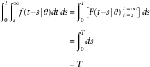 $$\eqalignno{ {\int}_0^T {{\int}_s^\infty {f(t{\minus}s\!\mid\!\theta )dt\,ds} } & \,{\equals}\,{\int}_0^T {\left[ {F(t{\minus}s\!\mid\!\theta )\!\!\mid_{{t\,{\equals}\,s}}^{{t\,{\equals}\,\infty}} } \right]\,ds} \cr & \,{\equals}\,{\int}_0^T {ds} \cr & \,{\equals}\,T $$
At time τ, assume that r=r(τ) events have been observed. We shall denote the ordered pair of occurrence time and reporting time by D j , that is, D j =(s j , t j ) where j=1, … , r(τ). Also, we shall denote by D(τ) the collective data on all events which are reported at time τ, that is, D(τ)={D 1, … , D r(τ)}. For the degenerate case r(τ)=0, D(τ) is then the empty set. Clearly, D(τ) are non-decreasing sets, so that D(τ 1)⊂D(τ 2) for τ 1≤τ 2, which means our knowledge of the process cannot decrease as time progresses. One of our aims is to predict the number of unreported events u(τ)=N(τ)−r(τ) at time τ, based on the information in D(τ).
2.1. The likelihood function
Recall that the IBNYR event process occurs in continuous time. We derive the likelihood of the observed process at time τ by conditioning on there being N(τ)=n events, and that r(τ) of these are known. Conditional on N(τ)=n, the likelihood for the observed data at time τ, denoted L τ , is
 $$L_{\tau } (D(\tau )\!\mid\!\theta ,n)\propto{{n\,!\,} \over {(n{\minus}r)\,!\,}}\left[ {\prod\limits_{j\,{\equals}\,1}^r {p(D_{j} \!\mid\!\theta )} } \right]\left[ {1{\minus}\Pi (\tau \!\mid\!\theta )} \right]^{{n{\minus}r}} $$
with
 $$p(D_{j} \!\mid\!\theta )\,{\equals}\,p(s_{j} ,t_{j} \!\mid\!\theta )$$
and
 $$\Pi (\tau \!\mid\!\theta )\,{\equals}\,\left\{ {\matrix{ {{1 \over T}{\int}_0^\tau {F(w\!\mid\!\theta )dw} \quad } & {\tau \leq T} \cr {{1 \over T}{\int}_{\tau {\minus}T}^\tau {F(w\!\mid\!\theta )dw} \quad } & {\tau \,\gt\,T} \cr } } \right.$$
Note that Π(τ|θ) represents the probability that an event will be reported before its observation time τ. Thus, 1−Π(τ|θ) is the probability that an event is unreported at time τ, and therefore, the probability that u=n−r events are outstanding/unreported at time τ is proportional to [1−Π(τ|θ)] n−r .
Let M=min{τ, T}. Given λ, N(τ) is Poisson(λM) by assumption that events are generated by a homogeneous Poisson process with rate λ over some fixed interval (0,T]. To see this, note that the exposure interval is (0,T], and so for τ≤T, N(τ)~Poisson(λτ); while for τ>T, N(τ)~Poisson(λT), since no events can occur after T.
We can therefore multiply (1) by a Poisson(λM) density to arrive at
 $$L_{\tau } (D(\tau )\!\mid\!\theta ,n){\times}p(n\!\mid\!\lambda )\propto{{n\,!\,} \over {(n{\minus}r)\,!\,}}\prod\limits_{j\,{\equals}\,1}^r {\left[ {p(D_{j} \!\mid\!\theta )} \right][1{\minus}\Pi (\tau \!\mid\!\theta )]^{{n{\minus}r}} } {\times}{1 \over {n\,!\,}}(\lambda M)^{n} e^{{{\minus}\lambda M}} $$
After simplification, we have
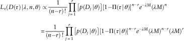 $$\eqalignno{ L_{\tau } (D(\tau )\!\mid\!\lambda ,n,\theta ) & \propto{1 \over {(n{\minus}r)\,!\,}}\prod\limits_{j\,{\equals}\,1}^r {\left[ {p(D_{j} \!\mid\!\theta )} \right]\left[ {1{\minus}\Pi (\tau \!\mid\!\theta )} \right]^{{n{\minus}r}} e^{{{\minus}\lambda M}} (\lambda M)^{n} } \cr & {\equals}{1 \over {(n{\minus}r)\,!\,}}\prod\limits_{j\,{\equals}\,1}^r {\left[ {p(D_{j} \!\mid\!\theta )} \right]\left[ {1{\minus}\Pi (\tau \!\mid\!\theta )} \right]^{{n{\minus}r}} e^{{{\minus}\lambda M}} (\lambda M)^{{n{\minus}r}} (\lambda M)^{r} } $$
and substituting u=n−r, yields
 $$L_{\tau } (D(\tau )\!\mid\!\lambda ,u,\theta )\propto{1 \over {u\,!\,}}\prod\limits_{j\,{\equals}\,1}^r {\left[ {p(D_{j} \!\mid\!\theta )} \right]\left[ {\lambda M(1{\minus}\Pi (\tau \!\mid\!\theta ))} \right]^{u} e^{{{\minus}\lambda M}} (\lambda M)^{r} } $$
By rearranging terms, we see that the last part is a Poisson density in terms of u. Thus
 $$L_{\tau } (D(\tau )\!\mid\!\lambda ,u,\theta )\propto e^{{{\minus}\lambda M}} \prod\limits_{j\,{\equals}\,1}^r {\left[ {p(D_{j} \!\mid\!\theta )} \right](\lambda M)^{r} {1 \over {u\,!\,}}\left[ {\lambda M(1{\minus}\Pi (\tau \!\mid\!\theta ))} \right]^{u} } $$
Integrating (3) with respect to u and simplifying, yields
 $$L_{\tau } (D(\tau )\!\mid\!\lambda ,\theta )\propto e^{{{\minus}\lambda M\Pi (\tau \mid\theta )}} \prod\limits_{j\,{\equals}\,1}^r {\left[ {p(D_{j} \!\mid\!\theta )} \right](\lambda M)^{r} } $$
Summarising, u(τ), the number of unreported events at observation time τ, has a Poisson distribution with parameter λM(1−Π(τ|θ)). This is not entirely surprising as we could also have derived this result using the colouring theorem for Poisson processes (see e.g. Kingman, Reference Kingman1993: 53). Note that, as is expected, the Poisson parameter for unreported events will tend to 0 as the observation time τ increases. The rate at which the parameter tends to 0, however, will be affected by the size of the right tail of the delay distribution (Figure 2).
Remark 1 Although some events can remain unreported for very long periods, the delay distribution is not usually long tailed. For example, asbestos claims can remain latent for decades and clearly, in this case, the delays are long tailed. However, it is generally accepted in the insurance industry that claims usually have smaller reporting delays.
Claims reporting process. Claims occur at some time s and are reported at some later time t. IBNYR, incurred but not yet reported.

The presentation given up to this point makes no restrictions on the delay parameter θ. However, for illustration purposes, we shall assume exponential delays. Thus, for Type I data
 $$p(D_{j} \!\mid\!\theta )\,{\equals}\,{1 \over T}\theta e^{{{\minus}\theta (t_{j} {\minus}s_{j} )}} \,{\equals}\,{1 \over T}\theta e^{{{\minus}\theta w_{j} }} $$
while for Type IV data
 $$p(D_{j} \!\mid\!\theta )\,{\equals}\,\Pi (\tau \!\mid\!\theta )\,{\equals}\,{1 \over T}{\int}_{(\tau {\minus}T)^{{\plus}} }^\tau {F(w\!\mid\!\theta )dw} $$
The reported events will be those for which t j ≤τ. For a Bayesian analysis, we place prior distributions on the parameters λ and θ. At time τ, the posterior density of the parameters λ and θ takes the form
 $$\pi _{\tau } (\theta ,\lambda \!\mid\!D(\tau ))\propto L_{\tau } (D(\tau )\!\mid\!\lambda ,\theta )p(\lambda )p(\theta )$$
where L τ (D(τ)|λ,θ) will be specified given the assumed data type.
3. The Jewell model
Jewell (Reference Jewell1989) formulates a basic, continuous-time Bayesian model for predicting the total number of unreported IBNYR claims arising in a given exposure interval, when only an incomplete number of such claims have been reported by some point in time, called the observation time/date. He assumes that events are generated by a homogeneous Poisson process with rate parameter λ (events/year) over some fixed exposure interval (0,T]. There is also a delay in the reporting of these events, and the waiting time is driven by a continuous distribution with parameter θ, which could be vector valued. The delay distribution is common to all claims.
In Jewell’s Bayesian formulation, the prior densities of
 $$\tilde{\lambda }$$
and
 $$\tilde{\theta }$$
are assumed to be independent, and the posterior parameter density, p(λ,θ|D), is not very revealing for any choice of priors. Information about these parameters are obtained through an experiment that observes all reported events r(t) in some observation interval (0,t], where t is continuous. Jewell therefore focusses on the prediction of the unreported claim count, u(t)=n(T)−r(t), conditioned on D, the amount of secondary data that is available, of which there are four types (I–IV) as shown in Table 1.
Secondary data type.

The unreported claim u has posterior density p(u|D), that takes the form
 $$p(u\!\mid\!D)\propto p_{\lambda } (u\!\mid\!D)p_{\theta } (u\!\mid\!D)$$
where p λ (u|D) and p θ (u|D) are occurrence/arrival and delay integrals, respectively, given by
 $$p_{\lambda } (u\!\mid\!D)\,{\equals}\,{{T^{u} } \over {u\,!\,}}{\int} {\lambda ^{{r{\plus}u}} e^{{{\minus}\lambda \:T}} p(\lambda )\:d\lambda } $$
and
 $$p_{\theta } (u\!\mid\!D)\,{\equals}\,{\int} {L(\theta \!\mid\!D)\left[ {K(\theta )} \right]^{u} p(\theta )\:d\theta } $$
where
 $L\left( {\theta \!\mid\!D} \right)\,{\equals}\,\prod\nolimits_{_{j} _{{\,{\equals}\,{\rm }1}} }^r {\left[ {p\left( {D_{j} \!\mid\!\theta } \right)} \right]} $
, the Kernel
 $K\left( \theta \right)\,{\equals}\,1{\rm }{\minus}{\rm }{\tau \over T}\Pi (t\!\mid\!\theta )$
and τ=min{t,T}.
With the choice of the Gamma (a, b) prior for
 $$\tilde{\lambda }$$
, the occurrence integral and predictive density reduce, respectively, to
 $$\eqalignno{ & h_{\lambda } (u\!\mid\!D)\,{\equals}\,{{\Gamma (a{\plus}r{\plus}u)} \over {u\,!\,}}\left( {{T \over {b{\plus}T}}} \right)^{u} \cr & {{p(u{\plus}1\!\mid\!D)} \over {p(u\!\mid\!D)}}\,{\equals}\,\left( {{{a{\plus}r{\plus}u} \over {u{\plus}1}}} \right)\left( {{T \over {b{\plus}T}}} \right)\left( {{{h_{\theta } (u{\plus}1\!\mid\!D)} \over {h_{\theta } (u\!\mid\!D)}}} \right) $$
which is the predictive density in recursive form. If θ is known exactly, then
 $$p(u\!\mid\!D)\,{\equals}\,{{\Gamma (a{\plus}r{\plus}u)} \over {u\,!\,}}\left( {{{T{\minus}\tau \Pi (t\!\mid\!\theta )} \over {b{\plus}T}}} \right)^{u} $$
which is a Pascal predictive density, with respective conditional mean and variance
 $$\eqalignno{ & {\bf E}(u\!\mid\!D)\,{\equals}\,{{(a{\plus}r)T} \over b}\left( {{{1{\minus}{\tau \over T}\Pi (t\!\mid\!\theta )} \over {1{\plus}{\tau \over T}\Pi (t\!\mid\!\theta )}}} \right) \cr & {\bf Var}(u\!\mid\!D)\,{\equals}\,{\bf E}(u\!\mid\!D)\left( {{{b{\plus}T} \over {b{\plus}\tau \Pi (t\!\mid\!\theta )}}} \right) $$
3.1. Gammoid approximation and Type III and IV data
When θ is unknown, the computation of the delay integral becomes more complex. Assuming that delays follow the familiar exponential distribution f(w|θ)=θe −θw , Jewell computes different likelihood depending on the type of data.
For example, Type I data have
 $$p(D_{j} \!\mid\!\theta )\,{\equals}\,{1 \over T}\theta e^{{{\minus}\theta w}} $$
while for Type IV data
 $$p(D_{j} \!\mid\!\theta )\,{\equals}\,\Pi (t\!\mid\!\theta )\,{\equals}\,{\tau \over T}{\minus}{1 \over {\theta T}}\left( {e^{{{\minus}\theta (t{\minus}T)}} {\minus}e^{{{\minus}\theta t}} } \right)$$
Jewell estimates the predictive density
 $$p_{\theta } (u\!\mid\!D)\,{\equals}\,{\int} {L(\theta \!\mid\!D)\left[ {K(\theta )} \right]^{u} p(\theta )\:d\theta } $$
using the Gammoid function g(θ)=(Aθ)Γ
e
−Δθ
to approximate the first two factors in the integral for p
θ
(u|D) above. This is achieved by assuming that the prior on the unknown delay parameter
 $$\tilde{\theta }$$
is Gamma (c
0, d
0), which has a mode at
 $$\theta _{0} \,{\equals}\,{{c_{0} {\minus}1} \over {d_{o} }}$$
. Approximations are centred around the mode of the integrand. This procedure converts the integral into a Gamma integral that is dependent on u. Jewell obtains excellent results with c
0=3 or 4 for Type I or II data. For Type III or IV data, he obtains the recursive formula for the predictive density as
 $${{p(u{\plus}1\!\mid\!D)} \over {p(u\!\mid\!D)}}\,{\equals}\,\left( {{{a{\plus}r{\plus}u} \over {u{\plus}1}}} \right)\left( {{T \over {b{\plus}T}}} \right)\left( {{{d_{0} {\plus}\Delta {\plus}\delta _{K} u} \over {d_{0} {\plus}\Delta {\plus}\delta _{K} {\plus}\delta _{K} u}}} \right)^{{c_{0} {\plus}\Gamma }} $$
where Γ and Δ are computed from the number of reported events, and
 $$\delta _{K} \,\approx\,{{t^{3} } \over {2T^{2} }},\:t\leq T$$
and
 $$\delta _{K} \,\approx\,t{\minus}{T \over 2},\:t\geq T$$
. Jewell’s model works very well for Types I and II. However, using Type IV data (count data only), a numerical example shows that the model gives a steady and dramatic increase in all the predictors as r increases (or t increases beyond the exposure interval), and the point estimators (mean and variance) grow without bound. Jewell posits that this happens because there is less and less information in Type IV data as t increases. This is also true for Type III data.
Jewell concludes that if the reporting dates of IBNYR claims are not available then Bayesian predictions, though mathematically correct, are operationally useless. This is because Type IV (or III) data are uninformative when the priors on
 $$\tilde{\lambda }$$
and
 $$\tilde{\theta }$$
are not sufficiently precise. Satisfactory stability in estimating the parameters and predicting the unreported claims require the observation of at least the reporting dates, that is, the time history of the reported claims, r(t).
We will show that when MCMC is applied, no such problems arise for Type III or IV data, which has the least information. Thus, the problems encountered by Jewell’s Gammoid approximation are completely circumvented when MCMC methods are used. This affirms Jewell’s claim that the Bayesian formulation is not the problem. However, we disagree with his conclusion that it is the lack of information that creates explosions in the estimators, but rather the approximation method that was employed.
4. MCMC Implementation
We now apply MCMC to the continuous-time IBNYR claims model of Jewell (Reference Jewell1989). A Gibbs sampling procedure is used to draw MCMC samples. We first develop the model for Type I data in detail, and implement it using MCMC. We then consider claims count only using Type IV data and demonstrate that our computational methods have a significant advantage over the Gammoid approximation of Jewell (Reference Jewell1989) for Type IV (or III) data. In a Bayesian setting where the likelihood function does not carry much information about the parameters of interest, the posterior distribution of such a parameter should revert to the prior distribution and should not become unboundedly large. In particular, we show that when MCMC methods are used, the likelihood function does not become unbounded when the data are Type IV. We illustrate the relative stability of the MCMC method versus the Gammoid approximation of Jewell (Reference Jewell1989) by showing that the MCMC estimates approach their prior parameters, while the Gammoid approximations grow without bound. Moreover, this holds for any distribution that the delay parameter follows. Our framework also allows for the computation of posterior confidence intervals for our parameters.
4.1. Simulations
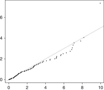
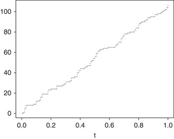
We implement the model using simulated data. Our data set have known parameters θ=0.5, λ=100 and T=1, for which the expected number of claims is λT=100. For this particular simulated data set, the observed number of claims is 107 and the mean inter-arrival time is 0.432−1=2.315 years (Figures 3 and 4).
QQ plot of the simulated inter-arrival times against the standard exponential. The dashed line has slope 1/2.

Step function plot of N(t) against t for our simulated data set.

Before presenting detailed results for Types I and IV data, note that for 0<τ≤T, we focus on the number of claims in [0,τ] which are unreported at time τ, while for τ>T, we focus on claims in [0,T] which are unreported at time τ. This is different from Jewell (Reference Jewell1989) who at any observation time τ>0 considers only unreported claims in the interval [0,T].
4.2. Claims with full reporting dates
For the Bayesian analysis, we use a Gamma (a 1, b 1) prior on λ and a Gamma (a 2, b 2) prior on θ. At time τ, given r=r(τ) reported claims, the joint posterior of λ and θ is
 $$\pi (\lambda ,\theta \!\mid\!D(\tau ))\propto\prod\limits_{\{ j\,\colon\,t_{j} \leq \tau \} } {\theta e^{{{\minus}\theta w_{j} }} (\lambda M)^{r} e^{{{\minus}\lambda M\Pi (\tau \mid\theta )}} p(\lambda )p(\theta )} $$
where we have removed the uninformative terms involving T, and
 $$\Pi (\tau \!\mid\!\theta )\,{\equals}\,\left\{ {\matrix{ {{\tau \over T}{\minus}{1 \over {\theta T}}\left[ {1{\minus}e^{{{\minus}\theta \tau }} } \right]} & {\tau \leq T} \cr {1{\minus}{1 \over {\theta T}}\left[ {e^{{{\minus}\theta (\tau {\minus}T)}} {\minus}e^{{{\minus}\theta \tau }} } \right]} & {\tau \,\gt\,T} \cr } } \right.$$
follows from (2) above, given exponential waiting times from occurrence to notification. The posterior conditional of λ is
 $$\eqalignno{ \pi _{\tau } (\lambda \!\mid\!\:\theta ,\:D(\tau )) & \propto L_{\tau } (D(\tau )\;\!\mid\!\:\lambda ,\:\theta )p(\lambda ) \cr & \propto\lambda ^{{a_{1} {\plus}r{\minus}1}} {\rm exp}\{ {\minus}\lambda (b_{1} {\plus}M\Pi (\tau \!\mid\!\:\theta ))\} $$
which is a Gamma (a 1+r, b 1+MΠ(τ|θ))) density. We also determine the posterior of θ at time τ
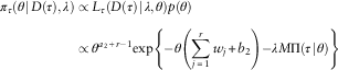 $$\eqalignno{ \pi _{\tau } (\theta \!\mid\!\:D(\tau ),\:\lambda ) & \propto L_{\tau } (D(\tau )\:\!\mid\!\:\lambda ,\:\theta )p(\theta ) \cr & \propto\theta ^{{a_{2} {\plus}r{\minus}1}} {\rm exp}\left\{ {{\minus}\theta \left( {\mathop{\sum}\limits_{j\,{\equals}\,1}^r {w_{j} {\plus}b_{2} } } \right){\minus}\lambda M\Pi (\tau \!\mid\!\theta )} \right\} $$
which is non-standard and so cannot be sampled from directly.
Remark 2 We note that this resembles a Gumbel distribution which has a long tail; the long-tailed nature of this distribution may contribute to the failure of the Gammoid approximation used by Jewel.
We propose a Gibbs updating scheme where each parameter is updated at each iteration. The updating is done via a Gibbs updating scheme with a single update random walk Metropolis sampler used for θ. For inference on u(τ), the number of unreported claims at time τ, we note that it is a Poisson random variable with parameter λM(1−Π(τ|θ))(see equation (3)). For any time τ, the updating proceeds as follows, given λ (i) and θ (i):
-
∙
 $$\lambda ^{{(i{\plus}1)}} \,\,\sim\,{\rm Gamma}\,\,\left( {a_{1} {\plus}r(\tau ),\,\,b_{1} {\plus}\Pi \,(\tau \!\mid\!\theta ^{{(i)}} )} \right)$$
-
∙
$$\theta ^{{(i{\plus}1)}} \,\sim\,\,\,\pi _{\tau } (\theta \!\mid\!\lambda ^{{(i{\plus}1)}} )$$
-
∙
$$u^{{(i{\plus}1)}} (\tau )\,\sim\,{\rm Poisson}\,\left( {\lambda ^{{(i{\plus}1)}} M(1{\minus}\Pi (\tau \!\mid\!\theta ^{{(i{\plus}1)}} ))} \right)$$
.



We follow Jewell (Reference Jewell1989) and choose a 1=2, b 1=0.02, a 2=4 and b 2=6. For our analysis, we do not estimate the parameters at time τ=0 since the number of claims at time 0 is 0 a.s.
Remark 3 Generally, we cannot obtain useful posterior estimates until at least one claim is known, since, in this case, no data are available, and we would simply be sampling from the prior distributions. If D(τ) is empty the likelihood should be defined to be equal to 1 since we would then be conditioning on an empty set. In this case, the posterior for λ and θ are their respective priors. So even though non-observation might have some information we cannot really update our beliefs about λ, the intensity of claims occurrence, which is not the same as claims observed.
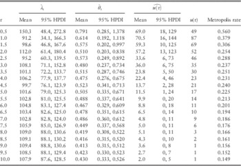
Table 2 shows how the posterior means of the parameters λ, θ and the unreported claims u(τ), change with time. Confidence intervals are shown in parentheses. The fourth column shows the actual number of unreported claims. Note that the number of unreported claims can increase or decrease with time since not all claims occur at time 0.
Posterior means of the model parameters as the observation time τ varies.

Note: The subscript τ, on λ and θ, indicates that the estimate was obtained using data reported up to that time.
HPDI, highest posterior density interval.
Based on the posterior analysis of the results in Table 2, the estimate of θ is decreasing with time. In particular, the posterior estimates of θ decreases from 0.791 to 0.430 as time increases. This is intuitive because claims with smaller delays tend to be reported first, and hence, our initial estimates of the delay time θ −1 will be small at first and will increase as time increases and more claims are reported. The estimate of the parameter θ, at time τ=10, is 0.430(0.048). This yields an average delay time of ~2.33 years, which is very close to 2.26 years, the average of the observed delay times.
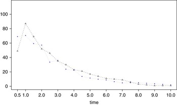
Figure 5 compares the posterior mean of the simulated values of u with the actual values at the times shown. Both quantities converge as time increases.
Plot of posterior mean of
 $$\widehat{{u(\tau )}}$$
against time (solid line). The figure also shows the actual number of unreported at the times given (dashed line).

4.3. Claims with no reporting dates
In this section, we illustrate the relative stability of the MCMC method versus the Gammoid approximation of Jewell (Reference Jewell1989). For type IV data, we have a count of the number of claims but no reporting dates. Thus for 1≤j≤r(τ), the density of the jth claim is
 $$\eqalignno{ p(D_{j} \!\mid\!\theta ) & \,{\equals}\,\Pi (\tau \!\mid\!\theta ) \cr & \,{\equals}\,{1 \over T}{\int}_{(\tau {\minus}T)^{{\plus}} }^\tau {F(w\!\mid\!\theta )dw} $$
which is just the probability that a claim is reported without knowing the actual dates. Substituting the above expression into (4) we get the joint posterior density of λ and θ
 $$\pi (\lambda ,\theta \!\mid\!D(\tau ))\propto p(\lambda )p(\theta )e^{{{\minus}\lambda M\Pi (\tau \mid\theta )}} (\lambda M)^{r} \prod\limits_{j\,{\equals}\,1}^r {\Pi (\tau \!\mid\!\theta )} $$
The posterior conditional density of λ is
 $$\eqalignno{ \pi (\lambda \!\mid\!\theta ,r) & \propto p(\lambda )L(D\!\mid\!\lambda ,\theta ) \cr & \propto\lambda ^{{a_{1} {\minus}1}} e^{{{\minus}b_{1} \lambda }} \lambda ^{r} {\rm exp}\{ {\minus}\lambda M\Pi (\tau \!\mid\!\theta )\} \cr & \,{\equals}\,\lambda ^{{a_{1} {\plus}r{\minus}1}} {\rm exp}\{ {\minus}\lambda (b_{1} {\plus}M\Pi (\tau \!\mid\!\theta ))\} $$
which we identify as the density of a random variable with a Gamma distribution. Likewise, θ has posterior density
 $$\eqalignno{ \pi (\theta \!\mid\!\lambda ,r) & \propto p(\theta )L(D\!\mid\!\lambda ,\theta ) \cr & \propto\theta ^{{a_{2} {\minus}1}} e^{{{\minus}b_{2} \theta }} \left[ {\Pi (\tau \!\mid\!\theta )} \right]^{r} \,{\rm exp}\{ {\minus}\lambda M\Pi (\tau \!\mid\!\theta )\} \cr & \propto\theta ^{{a_{2} {\minus}1}} \left[ {\Pi (\tau \!\mid\!\theta )} \right]^{r} {\rm exp}\{ {\minus}(b_{2} \theta {\plus}\lambda M\Pi (\tau \!\mid\!\theta )\} $$
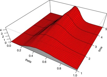
Remark 4 A representation of equation (8) is displayed in Figure 5 which shows the joint posterior distribution of (θ,τ). We highlight the posterior density of θ versus τ. As τ increases, the dispersion of θ decreases markedly, while its mean increases steadily. Moreover, the density of θ is long tailed for each fixed τ. However, its peakedness increases while the thickness of its tail and skewness decrease as τ increases.
We agree with Jewell (Reference Jewell1989) that there is less and less information in Type IV data as τ increases (Figure 6). To see this, note that as τ increases Π(τ|θ) → 1 and from (8) we see that π(θ|λ) → p(θ), the prior density of θ, for any λ. In the next section, we show that whereas the MCMC estimates approach the prior parameters, the Gammoid approximations grow without bound! It is interesting to note that the above argument holds for any inter-arrival distribution that θ is assumed to follow.
Plot showing the posterior density of θ as τ increases from τ=1 to τ=5. As τ increases, and more information is contained in the process D(τ), the estimate of θ shows less dispersion around its mean value.

4.4. Comparison of results
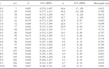
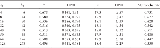
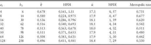
Setting a 1=2, b 1=0.02, a 2=4, b 2=6, we run the MCMC algorithm and then compare our results with those of Jewell (Reference Jewell1989). The results for Type IV data are summarised in Tables 3 and 4. Here we focus on θ, since from (7), we see that the posterior conditional of λ is the same as for Type I data given in equation (6).
τ versus θ, a 1=2, b 1=0.01, a 2=4, b 2=6.

Note: HPDI, highest posterior density interval.
Prior sensitivity, τ=4T.
Note: HPDI, highest posterior density interval.
Our Table 3 is analogous to table 2 in Jewell (Reference Jewell1989). Table 3 shows the changes in the parameter estimates as τ increases. As our previous discussions suggest, as τ increases there is less information contained in the likelihood function. In this case, the prior dominates and the posterior density of θ should be asymptotically equal to the prior density. While this is intuitive, the estimates based on Gammoid approximations grow without bound as τ increases.
Our results are also sensitive to the prior information assumed on the delay parameter θ. Moreover, they show that with even relatively uninformative priors, our algorithm converges quite easily in some cases where the Gammoid approximations give poor estimations. This is contrary to what is reported in Jewell (Reference Jewell1989). In fact, our estimates stabilise as τ increases, whereas those based on the Gammoid approximations grow without bound. Thus, we see that the MCMC method can offer computational advantages over the poor approximation of Jewell. Table 4 shows the effect of prior assumptions on the parameter estimates as a 1, b 1, a 2 and b 2 change.
Our results also show that stability is more sensitive to choices of a 2 and b 2 than on values of a 1 and b 1; that is, if p(θ) is informative then p(λ) can be diffuse without affecting the results.
The values of a 2 and b 2 were chosen so that the mode (a 2−1)/(b 2), of the Gamma prior is the same as the known value θ, hence the (maximum likelihood) estimates would approach the true value of θ. In Table 4, we exclude the case where both a 2 and b 2 are infinitely large.
Another important point to note is that for any choice of inter-arrival distribution time as τ → ∞ Π(τ|θ) → 1 and thus we are sampling from the prior on θ. This is also the case for Type I and Type II data.
5. Summary and Discussion
5.1. Motivating the Gammoid approximations
Jewell (Reference Jewell1989) shows that there is no maximum likelihood estimator of λ and θ in the case of Type IV data, and hence no estimator of the number of unreported claims. By assuming a Bayesian formulation however, a solution in terms of Gammoid functions was shown to be possible. The total number of unreported claims at time τ has a Poisson distribution with rate parameter λ[T−MΠ(τ|θ)], where M=min{τ,T}. This rate is bounded above by λT[1−Π(T|θ)] which is the rate used in Jewell (Reference Jewell1989) when the observation time τ≥T. This includes two types of unreported claims; the first being all which have already occurred and are unreported, and all which are yet to occur. Assuming Gamma priors on θ and λ, it can then be shown that the posterior marginal distribution of u can be approximated by a Gamma-type integral. However, some approximation must be made to obtain the parameters of this Gamma integral. Full details can be found in Jewell (Reference Jewell1989).
5.2. MCMC
A natural method for the computation of the posterior quantities λ and θ, and hence also the prediction of unreported claims u, is the MCMC algorithm. In addition to posterior estimates, we are able to compute posterior confidence intervals and determine how useful the Bayesian formulation is. We implemented the model assuming all of our data are of type IV (i.e. no reporting dates or occurrence dates are known) and examined how the choice of the parameters a 2 and b 2 that generate the prior θ affects the outcome. When no information is contained in the likelihood function, the prior should dominate the likelihood. This is clear from our analysis. However, with the Gammoid approximations this is not the case, except where the priors are very informative. Our primary conclusion is that in any Bayesian analysis with the absence of an informative likelihood, the prior distribution dominates the likelihood function; also the prior information presents our best available knowledge about the parameters of interest. Another interesting fact is that these conclusions hold for any waiting time/delay distribution. The type of information available does not affect the estimate of λ, the arrival parameter.
5.3. Assessing convergence of the MCMC algorithm
All our results are based on running the Gibbs algorithm for 100,000 iterations after a burn in of 100,000. To assess convergence we use the method of Gelman (Reference Gelman1996). Since we are looking at a continuous-time model, we have to assess convergence for each t that we choose to estimate the model parameters. The last column in each of Tables 2–4 shows the Metropolis acceptance rates for θ.
5.4. Possible extensions to the model
The basic result presented here is that IBNYR events, such as claims, have a Poisson distribution with a reduced arrival parameter if event arrivals are Poisson distributed. This is not entirely surprising and we could also have derived the result using the colouring theorem for Poisson processes (see e.g. Kingman, Reference Kingman1993: 53). There are a plethora of settings where the model can be applied to estimate the true values of the events generating and delay parameters, and then to predict the number of events that are unreported. Typical examples are insurance claims, number of persons infected by an epidemic/disease, the impact of a drug on mortality rate, products under warranty, murders committed by a serial killer or gang, rapes, financial frauds, survey sampling by mail and undetected bugs in computer software.
The model could be extended to incorporate event costs such as claim size/severity, and also letting the parameters θ and λ be time dependent. In this context, let us now introduce a random variable X for the cost/claim size/severity. Thus, each event is now an ordered triple (s, t, X), where s is the occurrence time, t the reporting date and X the unreported costs (e.g. claim size). One possible extension is to model the joint density of (s, t, X) as
 $p(s,t,X)\propto f\left( {{\textstyle{{t{\minus}s} \over {\kappa X^{\alpha } }}}\!\mid\!\:\lambda ,\theta ,\xi } \right)$
, where λ, θ and ξ are unknown model parameters. The development then proceeds analogously: conditional on time and the model parameters, we derive the likelihood which we can then use for inference. Other forms might allow for more general inhomogeneous Poisson processes such as Markov-modulated Poisson processes.
Acknowledgements
Garfield O. Brown would like to acknowledge the financial support of the Cambridge Commonwealth Trust. Winston S. Buckley would like to thank Nathan Carter, Charles Hadlock and Lucy Kimball for their support and encouragement.