1. Introduction
During the last decades, the research and industry in mobile robots have addressed too many applications, such as medical, agricultural, services, search, rescue, personal, environmental monitoring, and other applications [Reference He, Bourne, Steiner, Mortensen, Hoffman, Dudley, Rogers, Cropek and Leang1−Reference Skorobogatov, Barrado and Salamí6]. The robot needs to interact with its static environment to achieve the required task through most applications. One objective for the robot in this interaction is to provide a collision-free path to reach the target endpoint to perform the task; this problem is known as robot path planning (RPP). The past decades have seen rapid development of different solutions in a dynamic environment that is more realistic for real-life applications. Where the obstacles, the target, or both are assumed to be moving in their environment which adds more complexity to the path planning [Reference Hoy, Matveev and Savkin7−Reference Mohanan and Salgoankar11].
Several attempts have been made to address the problem of RPP in a dynamic environment, among them: the artificial potential field approaches (APF), graph-based approaches, velocity-based approaches, configuration space-based approaches, probability-based approaches, artificial intelligence-based approaches, and hybrid approaches. The hybrid approaches maximize the benefits by using one or multiple methods mentioned above to solve the problem. Applying these different techniques to the autonomous robot depends on several factors, such as the complexity of the robot platform model, the robot surrounding environment: two or three dimensional (2D or 3D), the provided information about obstacles by the sensors, obstacles sizes and shapes, uncertainty, and the computational requirements [Reference Mohanan and Salgoankar11−Reference Goerzen, Kong and Mettler13]. For instance, autonomous quadrotors are one category of unmanned aerial vehicles (UAV); this system requires a fast update rate due to its fast dynamics with size and weight constraints. These limitations affect the type of used sensors in the UAV platform, and consequently, the type and availability of the known information about the surrounding environment are influenced [Reference Skorobogatov, Barrado and Salamí6, Reference Hoy, Matveev and Savkin7]. Several path planning approaches are investigated within 2D and 3D environments based on APF. These APF proposed approaches in the literature are categorized as the potential field, the potential guided, harmonic potential function, wavefront expansion, and intelligent potential field [Reference Jaradat, Garibeh and Feilat10−Reference Scherer, Singh, Chamberlain and Saripalli14]. The APF was utilized in ref. [Reference He, Bourne, Steiner, Mortensen, Hoffman, Dudley, Rogers, Cropek and Leang1] to provide collision-free navigation of autonomous chemical-sensing quadrotor for environmental monitoring in a 3D environment with stationary obstacles and a given altitude. Fluid motion planner is extended for 3D nonholonomic vehicles [Reference Lau, Eden and Oetomo15]; the approach is based on an extended APF for motion planning to deal with 3D environments with fixed target point. In this approach, a differential equation of fluid flow is used to accomplish the desired path.
A hybrid APF with velocity synthesis algorithm is deployed for mobile robot navigation in 3D for an underwater vehicle with fixed target point [Reference Cheng, Zhu, Sun, Chu, Nie and Zhang16]; this approach is dedicated to dealing with underwater environments. In ref. [Reference Zhuoning, Rulin, Zongji and Rui17], a path planning approach using a fuzzy virtual force (FVF) is proposed. The approach deals with the robot as a particle point moving in a 3D environment which moves under the influence of an adaptive path planning approach to reach a fixed target point. Compared to the
 $A^*$
approach, the demonstrated performance simulation for the FVF approach showed a good fast path planning. A 3D collision avoidance approach based on potential field for small scale helicopter is proposed in ref. [Reference Paul, Krogstad and Gravdahl18]; the approach is deployed for formation application of grouped helicopter based on the simulation platform. A mobile RPP in a dynamic environment is proposed in ref. [Reference Yin and Yin19]; the approach mainly considers the relative position, velocity, and acceleration between the robot, the target, and the obstacle, and the approach is proposed to overcome the limitations in stationary approaches for path planning in 2D. A real-time target tracking in a 3D dynamic environment is proposed in ref. [Reference Yao, Wang and Su20]. The approach is developed to integrate two high-level techniques: the Lyapunov Guidance Vector Field method and the collision avoidance implemented based on the fluid flow approach. Another hybrid approach is presented in ref. [Reference Dong, Chen, Zhou and Zhang21]. In this approach, the path planning problem is solved by combining the virtual force approach with a search algorithm mainly
 $A^*$
for a fixed target point in a 2D environment. In ref. [Reference Budiyanto, Cahyadi, Adji and Wahyunggoro22], a potential filed approach is applied to multiple UAVs in a dynamic environment. In this research, each UAV has its attractive force to the target. Simultaneously each UAV is considered as an obstacle to the other UAVs, which should repulse away using another force function; the approach addressed the solution based on 2D environment at a given altitude for the UAV. A fluid-based approach is developed in ref. [Reference NanWang and JunWang23]; the proposed system mainly contains two layers to provide an optimal path for an unmanned ground vehicle in a 2D environment. A potential field approach is implemented in ref. [Reference Huang and Low24] to find the optimal path for UAVs. The approach is implemented to find the optimal safe, efficient, and smooth trajectory for the UAV at a given altitude using data from a 3D environment. An optimal potential field approach for multi-UAVs is addressed in ref. [Reference Sun, Tang and Lao25]; the approach is implemented based on a distance factor and a jumping technique to overcome common practical problems in other approaches.
A grid-based fuzzy approach is presented in ref. [Reference Shi, Li, Pan, Hwang and Li26]. A 3D fuzzy grid map is implemented to enhance the overall calculations using: 2D dual grid maps, the identifier, and the height maps. The collision-free path is generated later based on the developed maps using navigation algorithm in 2D environments. An implementation for a potential field approach for an unmanned water surface vehicle is presented in ref. [Reference Schofield, Wilde and Murphy27], using three different potential fields as constant, linear, and exponential to control the vehicle while approaching the target for rescue applications. A new method for path planning and obstacle avoidance problem of intelligent robots based on deep Q-learning with experience replay and heuristic knowledge is presented in ref. [Reference Jiang, Huang and Ding28].
A nonlinear tracking control method for Cushion robot based on fuzzy path planning with safe angular velocity is introduced in ref. [Reference Sun and Yu29]. A new strategy based on the potential field method to make the optimal control of multi-UAVs in target tracking and cooperative competition is presented in ref. [Reference Yang, Liao, Yang and Li30]. Another improved potential field for navigation in a dynamic environment is presented in ref. [Reference Chuan-ling, Jing and Jing-yu31]; the approach is developed based on the mobile robot position, velocity, acceleration, and size. The relative position and acceleration are considered in defining the potential function in the 2D environment. In ref. [Reference Liang, Liu, Song and Hao32], the relative position and velocity between the mobile robot, the dynamic target, and the obstacles are involved in defining the final potential function for path planning in 2D environments. In ref. [Reference Morais, do Nascimento, Brito and Basso33], a 3D anticollision-based APF method for mobile robots is presented. In addition, an RGB-D sensor is used to detect the obstacles. In this approach, the mobile robot can pass between closely spaced obstacles with very minimum oscillations. A new approach to plan the path of robots in dynamic and stationary environments using potential field method and genetic algorithm is presented in ref. [Reference Albaghdadi and Ali34]. A fuzzy optimal time-variant APF for controlling a mobile robot is proposed in ref. [Reference Macktoobian and Shoorehdeli35]. The approach provides path planning for the mission considering the changing characteristics for the shadows of the obstacles in 2D environments. A multipoint potential field approach for underwater vehicle path planning in a 3D environment is introduced in ref. [Reference Saravanakumar and Asokan36]; the approach utilizes a discrete space by equiangular points in the direction of robot motion. The robot moves in the direction of the point with minimum potential, and the paper introduces 3D motion planning systems for UAVs in the water. A real-time path planning for a mobile robot in an unknown 2D environment is proposed in ref. [Reference Sfeir, Saad and Saliah-Hassane37]. The work is intended to reduce the oscillations and conflicts if the obstacle is close to a fixed target.
In ref. [Reference Sabudin, Omar, Joret, Ponniran, Sulong, Kadir and Debnath38], the APF was improved with path pruning to achieve an optimal path for a mobile robot in an unknown 2D environment. The fractional repulsive potential is introduced in ref. [Reference Receveur, Victor and Melchior39] for a mobile ground vehicle to obtain an optimal trajectory in an unknown 2D environment. Another dynamical fractional repulsive potential was introduced in ref. [Reference Ruiz, Victor, Melchior and Chaumette40] for a mobile vehicle in a 3D environment with a fixed target. Deploying the potential field approach for mobile robot forming in a 2D dynamic environment was proposed in ref. [Reference Zhang, Gao, Xie and Liu41]. A hybrid dynamic path planning of mobile robots in a complex 2D environment was proposed in ref. [Reference Ravankar, Ravankar, Emaru and Kobayashi42]; the approach combines the APF with probabilistic roadmaps to implement a hybrid path planning approach.
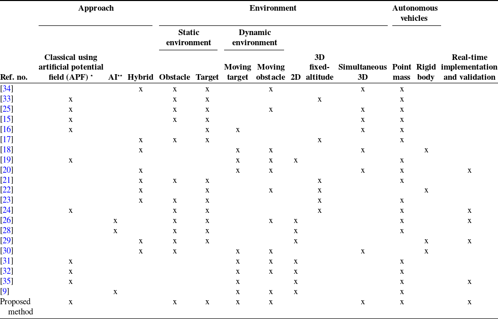
The majority of these potential field-based approaches were deployed in 2D stationary environments. For applying it to a dynamic environment, additional modification to the potential field forces and implementation efforts are required [Reference Hoy, Matveev and Savkin7, Reference Jaradat, Al-Rousan and Quadan9−Reference Goerzen, Kong and Mettler13]. The new environment requirements may be handled by augmenting additional factors or terms to the stationary relations, such as the relative positions and velocities. Such modifications may affect the computational and practical costs of the proposed approaches in 2D environments. Moreover, additional limitations should be considered for extensions of these approaches to the motion planning in 3D environments, such as model complexity, computational load, and the provided information from the perception process. These factors can affect the practical implementation of motion planning in real time [Reference Skorobogatov, Barrado and Salamí6, Reference Shi, Li, Pan, Hwang and Li26, Reference Liang, Liu, Song and Hao32]. 2D models were proposed to be used at different altitude positions in 3D environments as a solution. Therefore, this research develops a systematic analytical implementation approach to extend the generalized potential field forces in the 3D dynamic environment for quadrotors motion planning systems and overcome the theoretical and practical implementation in 3D environments. In this system, the quadrotor is considered to be moving under the influence of attractive and repulsive forces in the 3D space simultaneously. As a result, the quadrotor can change its altitude and projected planner position concurrently. Table I shows a detailed comparison between research works in the literature discussed above and the detailed work in this paper. This comparison table demonstrated that this research provided a real-time path planning implementation and validation of a simultaneous 3D-dynamic environment for an autonomous vehicle using APF when both target and obstacles are moving. This paper provides a set of simulations and experiments conducted to verify the motion planning systems’ validity and performance in a 3D dynamic environment.
Comparison of the literature research with the proposed approach.

* Includes artificial potential field (APF) approaches using mathematical models.
** Includes artificial potential field (APF) approaches using computational intelligence models such as fuzzy logic, neural network, or genetic algorithm.
The main objectives of this paper are summarized as follows:
-
To develop a systematic analytical solution of the potential filed approach for simultaneous path planning in a 3D dynamic environment.
-
To provide a simple solution of the local minima problem (LMP) in the potential filed path planning in static and dynamic environments.
-
To study the stability and the convergence of the developed method.
-
To perform statistical analysis of the developed approach and highlight its capability.
-
To implement and validate a real-time simultaneous path planning in 3D-dynamic environment of an autonomous vehicle using APF when both target and obstacles are moving.
The paper is organized as follows, after the introduction Section 1. The 3D extended potential force system is covered in Section 2. The local-Minima problem in the 3D dynamic environment is discussed Section 2.2. While the system’s validation based on simulations and real-time experiments are demonstrated in Sections 4 and 5, respectively. Finally, the conclusions are summarized in Section 6.
2. Potential field in 3D space
Oussama Khatib initially introduced the potential field approach for the manipulator robot’s path planning problem [Reference Khatib43]. Later, this method has been used for mobile robot navigation as well. The main idea and philosophy of the potential field approach are outlined as follows: The mobile robot moves in its environment while this environment can be described as a field of forces. The goal destination of the robot is an attractive force that pulls the robot toward it. At the same time, the obstacles are repulsive forces that push the robot away. The net potential force is the algebraic sum of these forces.
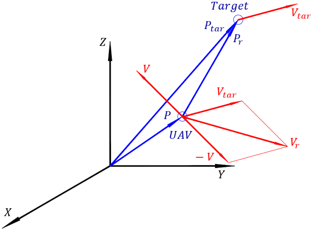
In this section, the derivations of the potential filed forces (repulsive and attractive forces) are presented to generate the potential field force for the UAV in a 3D dynamic environment. In this research, the UAV, the obstacles, and the target are not stationary and moving with constant velocities. The UAV is considered as a point-mass where its position in the workspace is denoted by
 $\vec{P}= R_x \ \hat{i}+ R_y \ \hat{j}+R_z \ \hat{k}$
, and the position vector of the target (destination)
 $\vec{P}_{tar}= T_x \ \hat{i}+ T_y \ \hat{j}+T_z \ \hat{k}$
. While, the velocity of the UAV and the target are
 $ \vec{V}= V_{rx} \ \hat{i}+ V_{ry} \ \hat{j}+V_{rz} \ \hat{k}$
and
 $\vec{V}_{tar}= V_{tx} \ \hat{i}+ V_{ty} \ \hat{j}+V_{tz} \ \hat{k}$
, respectively. As a result,
 $\vec{P}_r$
and
 $\vec{V}_r$
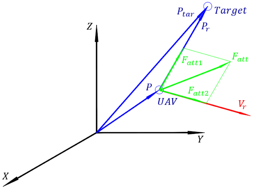
are the relative position and velocity vectors between the target and the robot, respectively. See Figs. 1 and 2.
 $P, P_{r}, P_{\textrm{tar}}, V, V_r, \textrm{and} \ V_{\textrm{tar}}$
for UAV tracking a moving target in a 3D space.

 $F_{\textrm{att}}, F_{\textrm{att}1}, \textrm{and} \ F_{\textrm{att}2}$
applied to UAV to track a moving target in 3D.

The following assumptions are imposed prior to starting the analyses [Reference Jaradat, Al-Rousan and Quadan9, Reference Jaradat, Garibeh and Feilat10, Reference Ge and Cui44]:
-
The target velocity and position are known all the time. Also, the target velocity is less than the UAV maximum velocity.
-
The obstacles position and velocity vectors are known all the time.
-
The UAV’s position and velocity vectors are known all the time.
2.1. Attractive potential force function in 3D space
The attractive force function is the gradient of the potential field function between the UAV and the target. The attractive force in 2D is defined by Ge and Cui [Reference Ge and Cui44]:
 \begin{equation} \vec{F}_{\textrm{att}}= \vec{F}_{\textrm{att1}}(P_r)+ \vec{F}_{\textrm{att2}}(V_r) \end{equation}
Equation (1) shows that the attractive force vector between the UAV and the target is the sum of two vectors. The
 $\vec{F}_{\textrm{att1}}$
vector depends on the relative position (The Euclidean distance
 $P_r = \|\vec{P}_{\textrm{tar}}(t)-\vec{P}(t) \|$
) between the robot and the target at any time. Equations (2) and (3) represent the mathematical form of
 $\vec{F}_{\textrm{att1}}$
. The
 $\vec{F}_{\textrm{att2}}$
is a function of the relative velocity between the robot and the target (
 $V= V_{\textrm{tar}}(t)$
-
 $V(t)$
), where
 $V_{\textrm{tar}}(t)$
,
 $V(t)$
are the velocities of the target and the UAV at time
 $t$
.
 \begin{equation} \vec{F}_{\textrm{att1}}(P_r)=m \ \alpha _{p} \left \|\vec{P}_{\textrm{tar}}(t)-\vec{P}(t)\right \|^{m-1} \ \vec{n}_{\textrm{RT}} \end{equation}
 \begin{equation} \vec{F}_{\textrm{att2}}(V_r)= n \ \alpha _{v} \|V_{\textrm{tar}}(t)-V(t)\|^{n-1} \ \vec{n}_{\textrm{VRT}} \end{equation}
The four positive scalar parameters
 $m,n, \alpha _p,$
and
 $ \alpha _v$
in Eqs. (2) and (3) need to be optimized based on the workspace size, the robot size and weight, and the speed of the robot as well as the target.
 $n_{\textrm{RT}}$
is the unit vector in the direction of the relative position vector between the target and the UAV. While
 $n_{\textrm{VRT}}$
is the unit vector in the direction of the relative velocity vector between the target and the UAV. Figures 1 and 2 provide a complete demonstration for the position and velocity for both the UAV as well as the target.
At any instance, the inverse of the directional cosine for the vectors
 $\vec{P_r}$
and
 $\vec{V_r}$
is used to get the angles between these two vectors and the three positive coordinate axes of the Cartesian coordinate. Where
 $\mathcal{L}_i$
represents the direction angle between the relative position vector
 $\vec{P_r}$
and the positive axes
 $i=\{x,y, z\}$
, and is defined by
 \begin{equation*} \label {reni} \mathcal {L}_i=\cos ^{-1}\left (\frac {\vec {P_r} \cdot \hat {e_i}}{\left \|P_{\text {r}}\right \| }\right ) \end{equation*}
where
 $\hat{e}=\{\hat{i}, \hat{j},\hat{k} \}$
is a unit vector in the direction of the three positive axes
 $\{x,y,z\}$
.
Also, the
 $\vec{F}_{\textrm{att2}}$
in the 3D space has the angles
 $\zeta _x$
,
 $\zeta _y$
, and
 $\zeta _z$
with the
 $x$
,
 $y$
, and
 $z$
axes. Where these angles are defined by
 \begin{equation*} \label {zetax} \zeta _i=\cos ^{-1}\left (\frac {\vec {V_r} \cdot \hat {e_i} }{\|V_{\text {r}}\|}\right ) \end{equation*}
As a result, Eqs. (2) and (3) can be rewritten in 3D space as
 \begin{equation} \left ( \begin{array}{c} F_{\textrm{att1x}} \\ F_{\textrm{att1y}} \\ F_{\textrm{att1z}} \\ \end{array} \right )=m \ \alpha _p\|P_r\|^{m-1}\left ( \begin{array}{c} \cos \left (\mathcal{L}_x\right ) \\ \cos \left (\mathcal{L}_y\right ) \\ \cos \left (\mathcal{L}_z\right ) \\ \end{array} \right ) \end{equation}
 \begin{equation} \left ( \begin{array}{c} F_{\textrm{att2x}} \\ F_{\textrm{att2y}} \\ F_{\textrm{att2z}} \\ \end{array} \right )=n \ \alpha _V \|V_r\|^{n-1}\left ( \begin{array}{c} \cos \left (\zeta _x\right ) \\ \cos \left (\zeta _y\right ) \\ \cos \left (\zeta _z\right ) \\ \end{array} \right ) \end{equation}
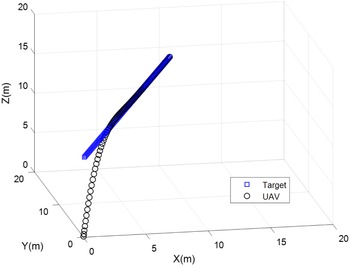
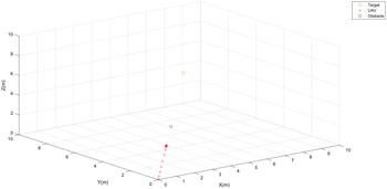
To validate the attractive force in 3D space, a simulation with no obstacles and moving target was conducted. As shown in Fig. 3, the UAV moves from the origin
 $ [ 0 \ 0 \ 0 ]^T$
with zero initial velocity, while the target moving in a straight line and constant velocity of
 $[ 0.1 \ 0.1 \ 0.1 ]^T \textrm{m/s}$
in the 3D space. The UAV tracks the target position, rendezvous with its motion, and lands safely on it after
 $47\; \textrm{s}$
. In this simulation, the performance for the attractive force was achieved using
 $m=n=2, \alpha _p=0.005, \alpha _v=0.1$
.
UAV tracking a moving target in 3D space using the new derived attractive force function.

2.1.1 Convergence and stability of the attractive potential force
To prove the converges of the UAV to the target, the UAV is set moving in the 3D space following a moving target influenced by attractive potential force. Then, the total attractive force applied to the UAV is expressed as follows:
 \begin{equation} F_{\textrm{att}}=m\alpha _p\left [P_{\textrm{tar}}-P\right ]{}^{m-1}+n\alpha _v\left [V_{\textrm{tar}}-V\right ]{}^{n-1} \end{equation}
Suppose that
 $F^*_{\textrm{UAV}}$
is the desired force to be applied to UAV to converge to the target and is expressed as follows:
 \begin{equation} F^*_{\textrm{UAV}}=a_{\textrm{tar}} m_{\textrm{UAV}}+F_{\textrm{att}} \end{equation}
Let
 $a^*_{\textrm{UAV}}$
be the desired acceleration when applying
 $F^*_{\textrm{UAV}}$
. So
 $F^*_{\textrm{UAV}} = m_{\textrm{UAV}} a^*_{\textrm{UAV}}$
, then by applying this equation and Eq. (6) into Eq. (7), the following equation is achieved:
 \begin{equation*}\label {StabilityEq3} a^*_{\textrm{UAV}} m_{\textrm{UAV}}=a_{\textrm{tar}} m_{\textrm{UAV}}+m\alpha _p\left [P_{\textrm{tar}}-P_{\textrm{UAV}}\right ]{}^{m-1}+n\alpha _v\left [V_{\textrm{tar}}-V_{\textrm{UAV}}\right ]{}^{n-1} \end{equation*}
Set
 $m_{\textrm{UAV}}=1\; \textrm{kg}, \;m =\;n=2$
, (the same parameters used in experiments and simulations) then recollecting the terms in the previous equation, we get
 \begin{equation*}\label {StabilityEq4} \left .[a_{\textrm{tar}}^*-a_{\textrm{UAV}}\right ]+2 \alpha _v\left (V_{\textrm{tar}}-V_{\textrm{UAV}}\right )+2 \alpha _p\left (P_{\textrm{tar}}-P_{\textrm{UAV}}\right )=0 \end{equation*}
Simplifying the terms in the previous equation, we get
 \begin{equation*}\label {StabilityEq5} \ddot {e}(t)+2 \alpha _v \dot {e}(t) + 2 \alpha _p e(t) =0 \end{equation*}
Taking Laplace for previous equation
 \begin{equation*}\label {StabilityEq6} S^2+ 2 \alpha _v S + 2 \alpha _p=0 \end{equation*}
Comparing the above equation to second-order general Laplace equation
 $ S^2+2\zeta \omega _n S+ \omega _n^2=0$
, we get the following two relations:
 \begin{equation*} 2\zeta \omega _n=2 \alpha _v \end{equation*}
 \begin{equation*} {\omega _n}^2=2 \alpha _{p} \end{equation*}
The system will be stable if both
 $\alpha _v\gt 0$
and
 $\alpha _p\gt 0$
. For instance, the system provides a critical damped system dynamic behavior such that UAV converges to the target without overshoot if
 $\zeta = 1$
hence
 $\omega _n= \alpha _v$
and
 $\alpha _v = \sqrt{2 \alpha _p}$
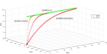
. To find the best values for
 $\alpha _{p}$
and
 $\alpha _{v}$
, three simulations were carried out for demonstration, Fig. 4. For large values of
 $\alpha _{p}$
and
 $\alpha _{v}$
, the system response is very fast, and the system response gets slower as the values of these two parameters are reduced. So the middle values were chosen.
UAV response for different values of (
 $\alpha _{p},\alpha _{v}$
).

2.2. Repulsive force function in 3D space
For obstacle avoidance in a dynamic environment, the repulsive force function between the robot and the obstacle is given by Eq. (8). As the robot starts approaching the influence range (IR) of the obstacle, the robot is affected by a repulsive force. This force depends on the relative position, and velocity between the robot and the obstacle [Reference Jaradat, Al-Rousan and Quadan9, Reference Jaradat, Garibeh and Feilat10, Reference Ge and Cui44]. Equations (8)−(26) show the detailed derivation of the repulsive force in 3D Space. In the case of more than one obstacle, the net repulsive force equals the sum of each repulsive force vector between the UAV and that obstacle.
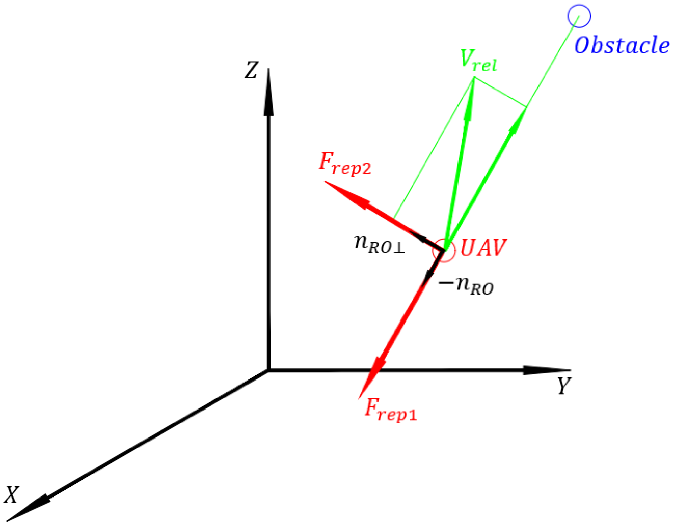
The repulsive force consists of two perpendicular forces (F
rep1 and F
rep2).
 $\vec{F}_{\textrm{rep}1}$
acts on a direction opposite to the relative position vector between UAV and obstacle where
 $\vec{F}_{\textrm{rep}2}$
acts on a direction perpendicular to
 $\vec{F}_{\textrm{rep}1}$
. The component
 $\vec{F}_{\textrm{rep}2}$
tries to move the UAV away from the obstacle and
 $\vec{F}_{\textrm{rep}1}$
tries to reduce its speed. That is why the value of
 $\vec{F}_{\textrm{rep}1}$
proportion to the relative velocity between the UAV and the obstacle (refer to Fig. 7).
 \begin{align} \vec{F}(p,v)_{\textrm{rep}}= \begin{Bmatrix} 0 & \textrm{if} \: \rho _s\left (p, p_{\textrm{obs}}\right )-\rho _m (v_{\textrm{RO}}) \geq \rho _o \\ \; & \textrm{and} \; v_{\textrm{RO}}(t)\leq 0 \\ \vec{F}_{\textrm{rep1}}+\vec{F}_{\textrm{rep2}} & \textrm{if} \: 0 \lt \rho _s\left (p,p_{\textrm{obs}}\right )-\rho _m (v_{\textrm{RO}})\lt \rho _o \\ \; & \textrm{and} \; v_{\textrm{RO}} \gt 0 \\ \textrm{not-defined} & \textrm{if} \: v_{\textrm{RO}}\gt \ 0 \ \\ \; & \textrm{and}\ \rho _s\left (p, p_{\textrm{obs}}\right )\lt \rho _m ( v_{\textrm{RO}}) \end{Bmatrix} \end{align}
where
 \begin{equation} \vec{F}_{\textrm{rep1}}=\frac{-\eta }{\left (\rho _s\left (p,p_{\textrm{obs}}\right )-\rho _m ( v_{\textrm{RO}})\right ){}^2} \left (1+ \frac{v_{\textrm{RO}}}{a_{\max }}\right ) \vec{n}_{\textrm{RO}} \end{equation}
and
 \begin{equation} \vec{F}_{\textrm{rep2}}=\frac{\eta \; v_{\textrm{RO}} \; v_{\textrm{RO} \bot }}{\rho _s\!\left (P,P_{\textrm{obs}}\right )a_{\max }\!\left (\rho _s\!\left(P,P_{\textrm{obs}}\right )-\rho _m (v_{\textrm{RO}})\right )^2} \vec{n}_{\textrm{RO}\bot } \end{equation}
where
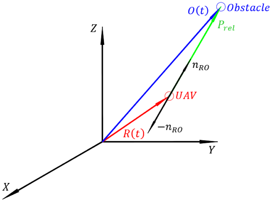
 $\vec{n}_{\textrm{RO}}$
is a unit vector in the direction of
 $\vec{P}_{\textrm{rel}}$
as shown in Fig. 5.
 $\vec{n}_{RO \bot }$
is also a unit vector perpendicular to the
 $\vec{n}_{\textrm{RO}}$
, as shown in Figs. 6 and 7.
Relative position vector between UAV and obstacle.

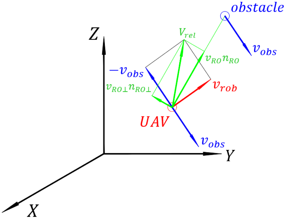
Relative velocity vector and its projection on
 $n_{\textrm{RO}}$
and
 $n_{\textrm{RO}} \bot$
vectors.

 $F_{\textrm{rep}1}$
and
 $F_{\textrm{rep}2}$
directions.

From Eqs. (9) to (10), the magnitudes of
 $\vec{F}_{\textrm{rep}1}$
and
 $\vec{F}_{\textrm{rep}2}$
depend on
 $v_{\textrm{RO}}$
,
 $v_{\textrm{RO} \bot }$
,
 $\rho _s$
, and
 $\rho _m$
. Where
 ${v_\textrm{RO}}$
is the projection of the relative velocity between UAV and obstacle vector to relative position between UAV and obstacle vector. Figures 5 and 6 show the relative position [
 $\vec{P} _{\textrm{rel}}=(O_x-R_x) \hat{i}+ (O_y-R_y) \hat{j} + (O_z-R_z) \hat{k}$
], and the relative velocity vector
 $[\vec{V}_{\textrm{rel}}= (V_{rx}- V_{ox}) \hat{i}+ (V_{ry}-V_{oy}) \hat{j} + (V_{rz}-V_{oz}) \hat{k}]$
between the UAV and the obstacle. Where [O
x
, O
y
, O
z
]
T
and
 $ [ R_x, R_y, R_z]^T$
are the location of the obstacle and the UAV, respectively.
 $ [V_{rx}, V_{ry}, V_{rz}]^T$
is the velocity vector of the UAV and
 $ [V_{ox}, V_{oy}, V_{oz}]^T$
is the velocity vector of the obstacle in the 3D space. Where
 $v_{\textrm{RO} \bot }$
is the projection of the relative velocity vector between UAV and obstacle to
 $n_{\textrm{RO}}\bot$
. While
 $ \rho _o$
is a positive constant describing the IR of the obstacle, and
 $\eta$
is a tuned positive constant that depends on the robot velocity. For detailed description of Eqs. (8)–(10) refer to ref. [Reference Ge and Cui44]. The angle
 $\theta$
, the angle between the two vectors
 $\vec{P}_{\textrm{rel}}$
and
 $\vec{V}_{\textrm{rel}}$
, is given by Eq. (11).
 \begin{equation} \theta = \cos ^{-1}\Biggl [ \frac{\vec{P}_{\textrm{rel}} \cdot \vec{V}_{\textrm{rel}}}{ \left \|P_{\textrm{rel}}\right \|\|V_{\textrm{rel}}\|} \Biggr ] \end{equation}
where
 $v_{\textrm{RO}}$
is the projection of the relative velocity (
 $\vec{V}_{\textrm{rel}}$
) to the relative position vector:
 \begin{equation} \|v_{\textrm{RO}}\|= \|V_{\textrm{rel}}\| \, \cos \left ( \theta \right ) \end{equation}
and
 \begin{equation} \|v_{\textrm{RO} \bot }\|= \|V_{\textrm{rel}}\| \, \sin \left ( \theta \right ) \end{equation}
Note that
 \begin{equation} \rho _m (v_{\textrm{RO}})=\frac{v_{\textrm{RO}}^2}{2 a_{\max }} \end{equation}
where
 $a_{\textrm{max}}$
is the maximum deceleration magnitude applied to the UAV to reduce its velocity, considered to be
 $1 \, \textrm{m}/{\textrm{s}}^2$
in this research.
 \begin{equation} \rho _s\left (\rho,\rho _{\textrm{obs}}\right )= \|P_{\textrm{rel}}\| \end{equation}
Recollecting the terms in Eq. (9), the magnitude of
 $\vec{F}_{\textrm{rep1}}$
is expressed as
 \begin{equation} \| F_{\textrm{rep1}} \| =\frac{\eta }{\left (\| P_{\textrm{rel}}\|-\frac{\left ( \| V_{\textrm{rel}}\| \cos \left ( \theta \right ) \right ){}^2 }{2}\right )^2 } * \left (1+ \| V_{\textrm{rel}}\| \cos \left ( \theta \right ) \right ) \end{equation}
where its directional angles are given by
 \begin{equation} \epsilon _i=\cos ^{-1}\left (\frac{-\vec{P}_{\textrm{rel}} \cdot \hat{e}_i}{\|- P_{\textrm{rel}}\|}\right ) \end{equation}
As a result,
 $F_{\textrm{rep}1x}$
,
 $F_{\textrm{rep}1y}$
, and
 $F_{\textrm{rep}1z}$
are rearranged as follows:
 \begin{equation} \begin{pmatrix} F_{\textrm{rep}1x}\\ F_{\textrm{rep}1y} \\ F_{\textrm{rep}1z}\\ \end{pmatrix} = ||F\textrm{rep}1||. \begin{pmatrix} \cos (\epsilon _x)\\ \cos (\epsilon _y) \\ \cos (\epsilon _z)\\ \end{pmatrix} \end{equation}
On the other hand, recollecting terms in Eq. (10) results in the magnitude of the
 $F_{\textrm{rep}2}$
as follows:
 \begin{equation} \|F_{\textrm{rep}2}\|=\frac{\eta{\|V_{\textrm{rel}} \|}^2 \sin (\theta ) \cos (\theta )}{\|P_{\textrm{rel}}\|(\|P_{\textrm{rel}}\|-\frac{1}{2}\|V_{\textrm{rel}}\|\cos (\theta ))} \end{equation}
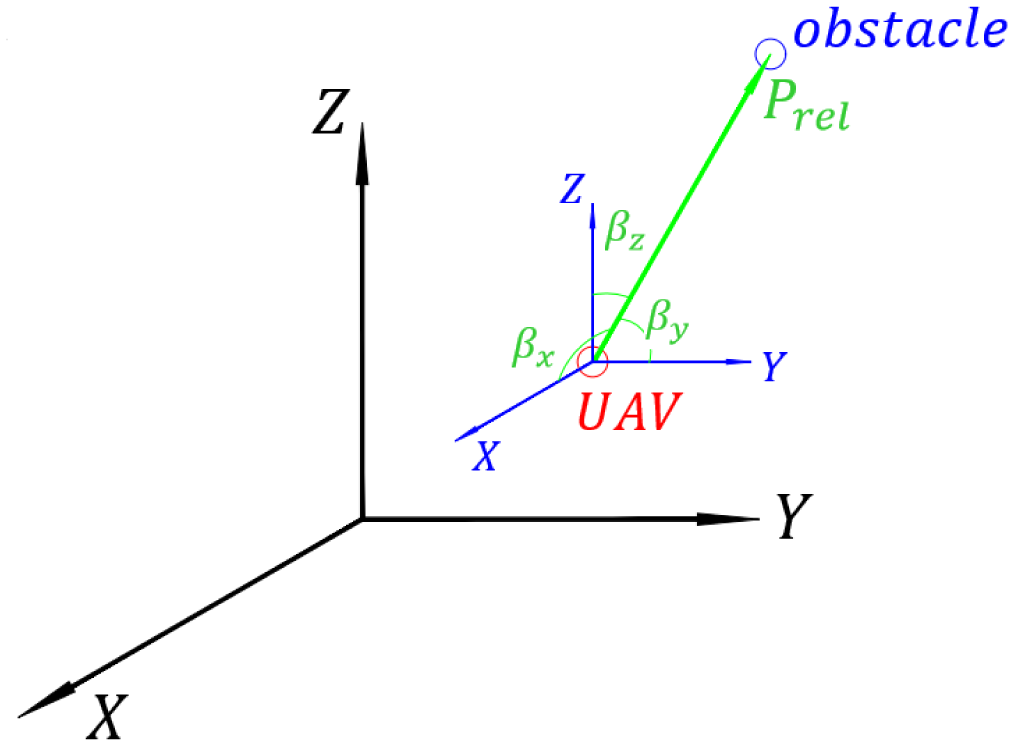
 $\beta _x$
,
 $\beta _y$
, and
 $ \beta _z$
angles.

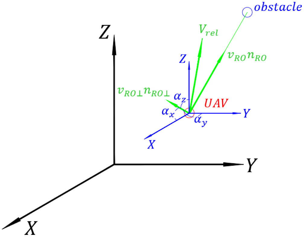
 $\alpha _x$
,
 $\alpha _y$
, and
 $ \alpha _z$
angles.

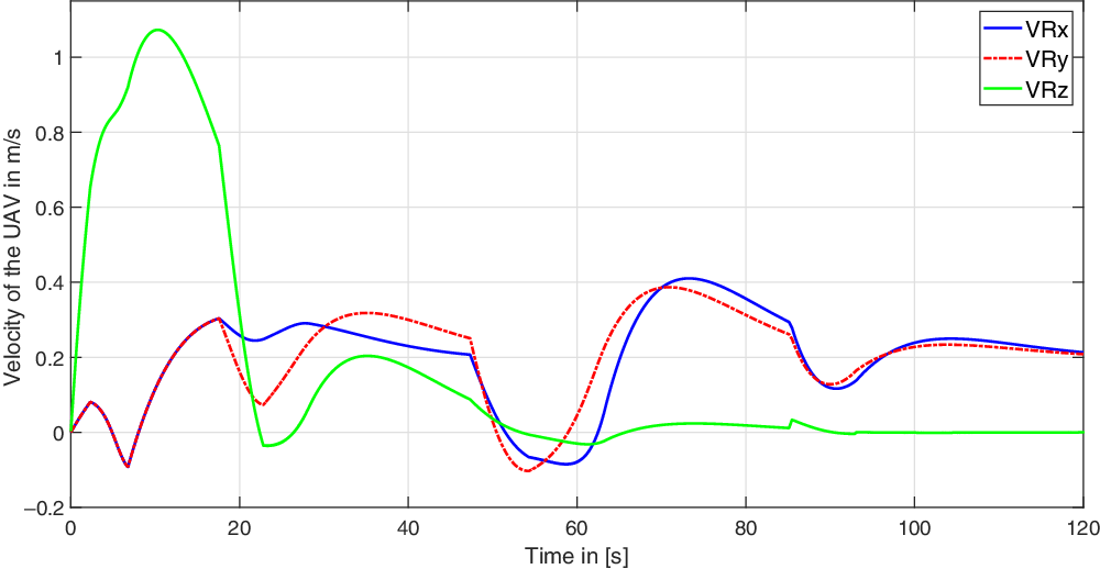
Velocity of UAV in x, y, z directions.

Path of UAV, obstacle1, obstacle2 at
 $t=50 \ [\textrm{s}]$
.

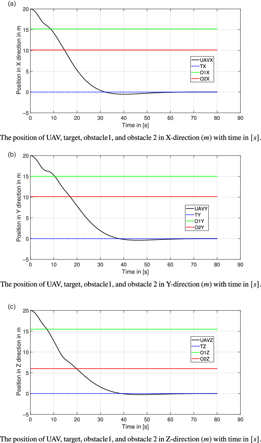
The position of the UAV, target, obstacle1, and obstacle2 with time.

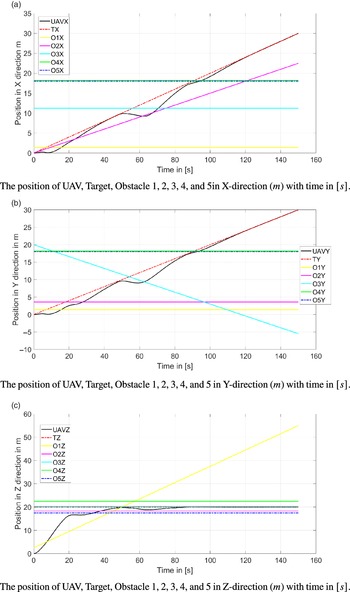
The position of the UAV, obstacle1, obstacle2,obstacle3, obstacle4, obstacle5, and Target.

The position of the UAV, Target, Obstacle1, and Obstacle2 with time.

Velocity of UAV in x, y, z directions.

LMP in static environment.

LMP in dynamic environment.

Explanation of LMP.

Solution of LMP in static environment.

Solution of LMP in dynamic environment.

The direction of
 $F_{\textrm{rep}2}$
is in the same direction of
 $v_{\textrm{RO} \bot }$
. To find the direction of
 $v_{\textrm{RO} \bot }$
, the direction of
 $v_{\textrm{RO}}$
is found which has the same direction of
 $\vec{P}_{\textrm{rel}}$
. Using the cosine law the angles between
 $\vec{P}_{\textrm{rel}}$
and
 $x,y, \ \textrm{and} \ z$
axes,
 $\beta _x,\beta _y, \ \textrm{and}\ \beta _z$
, are given in Eq. (20), as in Fig. 8. These angles are the same angles between
 $v_{\textrm{RO} }$
vector and the
 $x,y, \ \textrm{and} \ z$
axes, so
 $v_{\textrm{RO} }$
vector is defined in Eq. (21). And the
 $v_{\textrm{RO} \bot }$
is given in Eqs. (22) and (23).
 \begin{equation} \beta _i=\cos ^{-1}\left (\frac{\vec{P}_{\textrm{rel}} \cdot \vec{e}_i}{\| P_{\textrm{rel}}\|}\right ) \end{equation}
 \begin{equation} \vec{v}_{\textrm{RO}}=\left \|v_{\textrm{RO}}\right \|( \cos \left (\beta _x\right ) \hat{i} + \cos \left (\beta _y\right ) \hat{j}+ \cos \left (\beta _z\right ) \hat{k}) \end{equation}
 \begin{equation} \vec{v}_{\textrm{RO}\bot }=\vec{V}_{\textrm{rel}} - \vec{v}_{\textrm{RO}} \end{equation}
 \begin{equation} \begin{split} \vec{v}_{\textrm{RO}\bot } = &( (V_{\textrm{rx}}-V_{\textrm{ox}})- \|v_{\textrm{RO}}\|\cos (\beta _x)) \hat{i}+\\ & ((V_{\textrm{ry}}-V_{\textrm{oy}})- \|v_{\textrm{RO}}\|\cos (\beta _y)) \hat{j}+\\ & ( (V_{\textrm{rz}}-V_{\textrm{oz}})- \|v_{\textrm{RO}}\|\cos (\beta _z)) \hat{k} \end{split} \end{equation}
 $\vec{V}_{\textrm{RO}\bot }$
has the same direction of
 $\vec{F}_{\textrm{rep}2}$
then
 $\alpha _x$
,
 $\alpha _y$
, and
 $\alpha _z$
are the angles between
 $\vec{F}_{\textrm{rep}2}$
and
 $x,y, \ \textrm{and} \ z$
axes. So
 $F_{\textrm{rep}2x}$
,
 $F_{\textrm{rep}2y}$
, and
 $F_{\textrm{rep}2z}$
are given by Eq. (24). Figure 9 illustrates the angles
 $\alpha _x,\alpha _y, \ \textrm{and} \ \alpha _z$
.
 \begin{equation} \begin{pmatrix} F_{\textrm{rep}2x}\\ F_{\textrm{rep}2y} \\ F_{\textrm{rep}2z}\\ \end{pmatrix} = ||F\textrm{rep}2||. \begin{pmatrix} \cos (\alpha _x)\\ \cos (\alpha _y) \\ \cos (\alpha _z) \\ \end{pmatrix} \end{equation}
where
 \begin{equation} \alpha _i=\textrm{cos}^{-1}\left [\frac{(V_{\textrm{ri}}-V_{\textrm{oi}})-\left \|v_{\textrm{RO}}\right \|\cos \left (\beta _i\right )}{\left \|v_{\textrm{RO}\bot }\right \|}\right ] \end{equation}
Thus, the total repulsive force is given by the vector equation as follows:
 \begin{equation} \vec{F}_{\textrm{rep}}= \vec{F}_{\textrm{rep}1}+\vec{F}_{\textrm{rep}2} \end{equation}
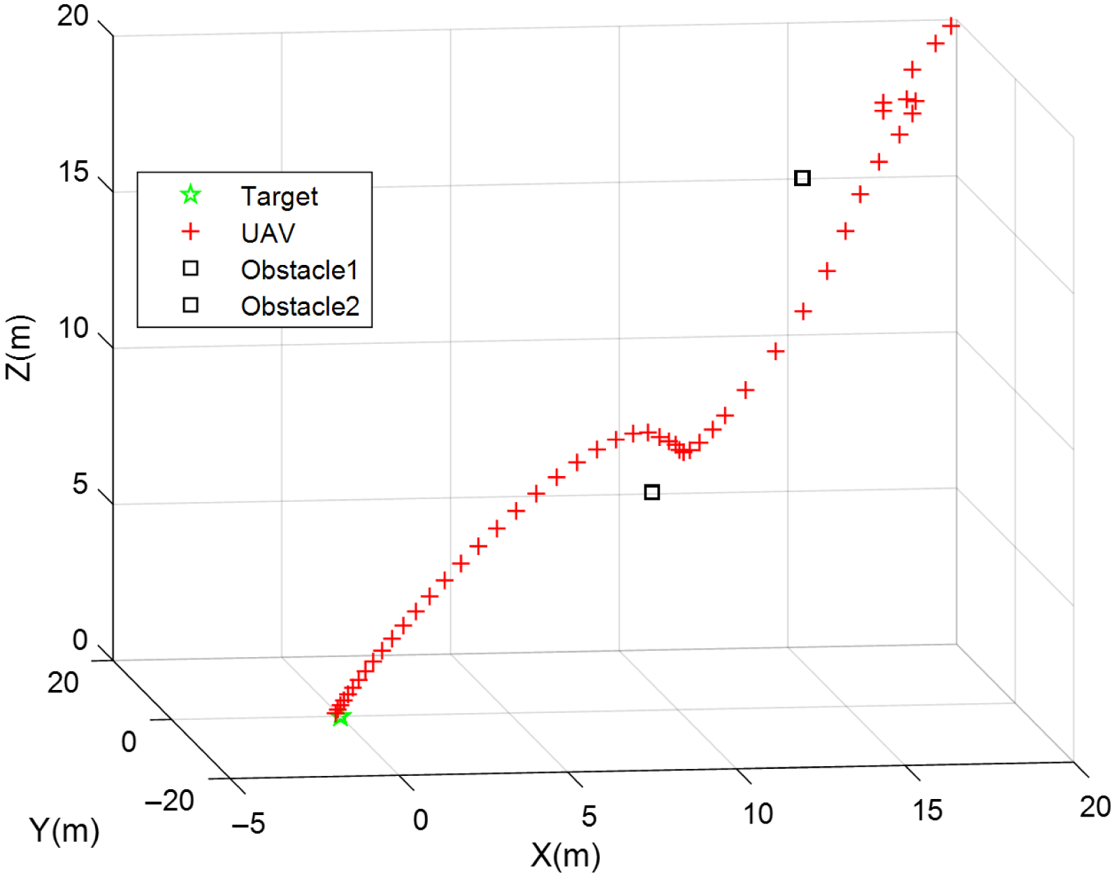
Two simulation studies were carried out to validate the derived attractive and repulsive forces. The first simulation study is presented to show the capability of the derived functions in the case of a static environment. Whereas the second simulation study deals with a highly dynamic environment. In both studies, the UAV was able to navigate smoothly away from the obstacles and reach the target safely. In the first simulation study (static environment), the first obstacle is located at position
 $[15 \ 15\ 15.3]^T$
, while the second obstacle is located at
 $[10.12\ 10.12 \ 6]^T$
, and the target is located at
 $[0 \ 0 \ 0]^T.$
The UAV starts its motion initially from point
 $[ 20 \ 20 \ 20 ]^T$
with zero initial velocity. At the time
 $t = 5 \ \textrm{s}$
, the UAV enters the IR of the first obstacle. The UAV continues to repulse away from the first obstacle until it reaches a point away from the obstacle’s IR at
 $t = 10 \ \textrm{s}$
. Then, the UAV moves toward the target until it approaches the second obstacle at
 $t = 19 \ \textrm{s}$
. As a result, the UAV starts to move away from the new obstacle until it gets away from its IR at
 $t = 33 \ \textrm{s}$
. Finally, the UAV successfully softly landed on the stationary target at
 $t = 50 \ \textrm{s}$
as shown in Fig. 11.
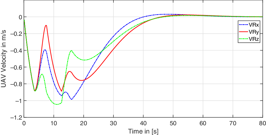
The x, y, and z-position components change with time of the UAV, the obstacles, and the target as shown in Fig. 12. The velocity components of the UAV are shown in Fig. 10. It is clear from the figure that the UAV reaches the target at time
 $t=50\ \textrm{s}$
, where its speed becomes zero.
The second simulation study is carried out to validate the derived forces of a dynamic environment in space. In this simulation, the UAV moves in a highly dynamic environment where five obstacles are involved and one moving target. The first obstacle starts its motion from point
 $[1.4 \ 1.4 \ 2.5]^T$
and moves with constant velocity of
 $[0 \ 0 \ 0.35]^T$
. The second obstacle starts its motion from point
 $[0 \ 3.56 \ 18.3]^T$
with a constant velocity of
 $[ 0.15 \ 0 \ 0 ]^T$
. The third obstacle moves in a constant velocity of
 $[0 \ -0.17 \ 0 ]^T$
from point
 $[ 11.2 \ 20 \ 20]^T$
. While the fourth and fifth obstacles are stationary and located at
 $[18 \ 18 \ 22.5]^T$
and
 $[18 \ 18 \ 17.5]^T$
, respectively. The target starts its motion from point
 $[0 \ 0 \ 20]^T$
with constant velocity of
 $[0 \ 0.2 \ 0.2]^T$
. On the other hand, the UAV starts its motion from the origin and with zero initial velocity.
Figure 13(a) shows that the UAV starts moving toward the target by the influence of the attractive force between the UAV and the target. At the time
 $ t = 3 \ \textrm{s}$
, the UAV started to get affected by the first obstacle. As a result, the UAV changed its path away from the obstacle until it gets away from the IR of the obstacle at time
 $t = 13 \ \textrm{s}$
.
Then at
 $t = 19 \ \textrm{s}$
, the UAV enters the IR of the second obstacle. So, it starts to repulse away from it until it gets out of the obstacle range at
 $ t = 32 \ \textrm{s}$
as shown in Fig. 13(b). Influenced by the attractive force, the UAV starts moving toward the target until it approaches the third obstacle at
 $ t = 52 \ \textrm{s}$
as shown in Fig. 13(c). Then, the UAV starts pulling away as shown in Fig. 13(d) at
 $ t = 70 \ \textrm{s}$
. At
 $ t = 95 \ \textrm{s}$
, the UAV starts approaching the IR of the stationary fourth and fifth obstacles and successfully passes between these two obstacles, see Fig. 13(e). Finally, the UAV successfully and softly landed on the moving target at
 $ t = 105 \ \textrm{s}$
, refer to Fig. 13(f).
Figure 14 shows the position components change with time of the UAV, the target, as well as the five obstacles. Figure 15 shows the magnitude of the velocity components changes with time of the UAV. From the two figures, it is clear that the robot reaches the target and they start moving with the same velocity.
System performance by increasing the number of obstacles in the operating space.

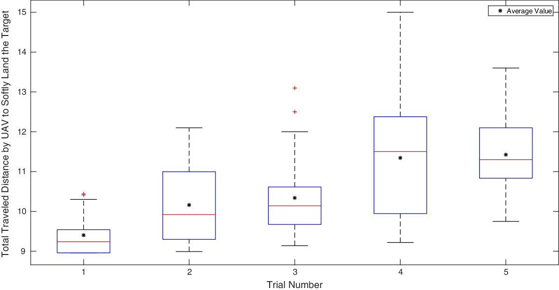
Simulation Result for total traveled distance of the UAV in the five trials, with 5, 10, 15, 20, and 25 obstacles.

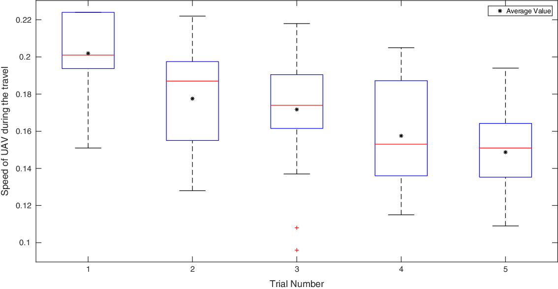
Simulation for the speed of the UAV in the five trials, with 5, 10, 15, 20, and 25 obstacles.

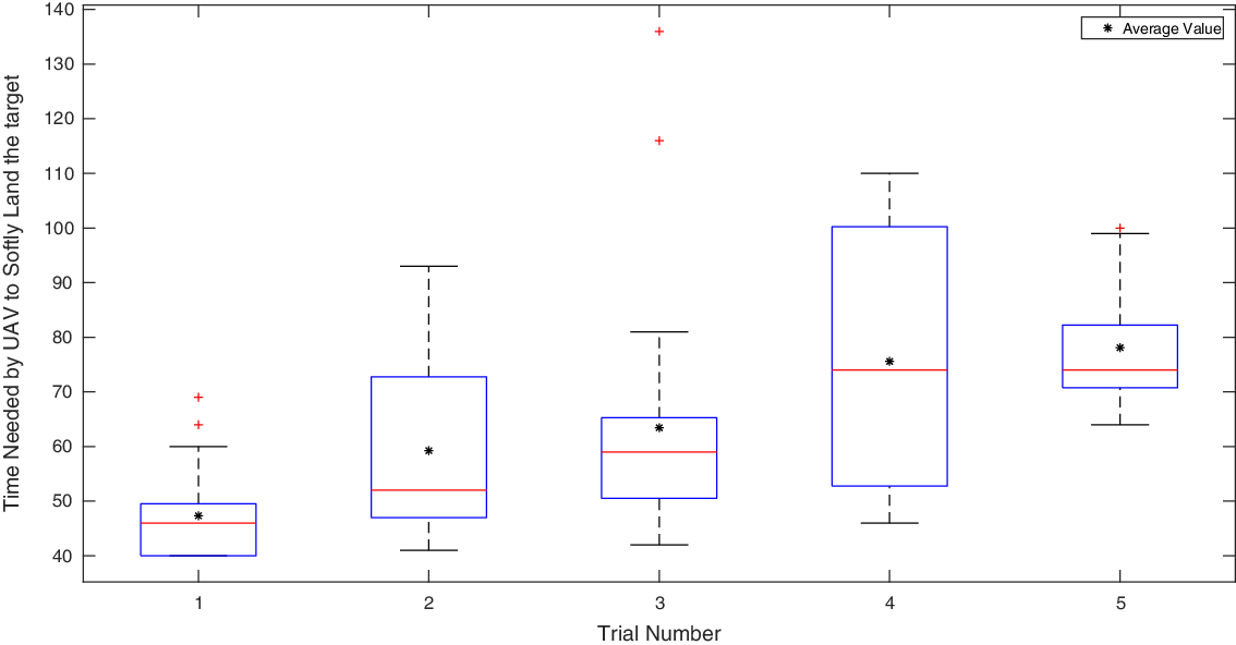
Simulation result of the time needed by the UAV to softly-land on the target, with 5, 10, 15, 20, and 25 obstacles.

Experimental setup.

Feedback control flowchart implemented on the onboard chasing drone.

Position tracks of the three vehicles in the 3D coordinates.

3. Local minima problem
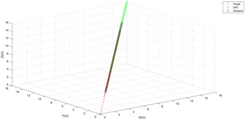
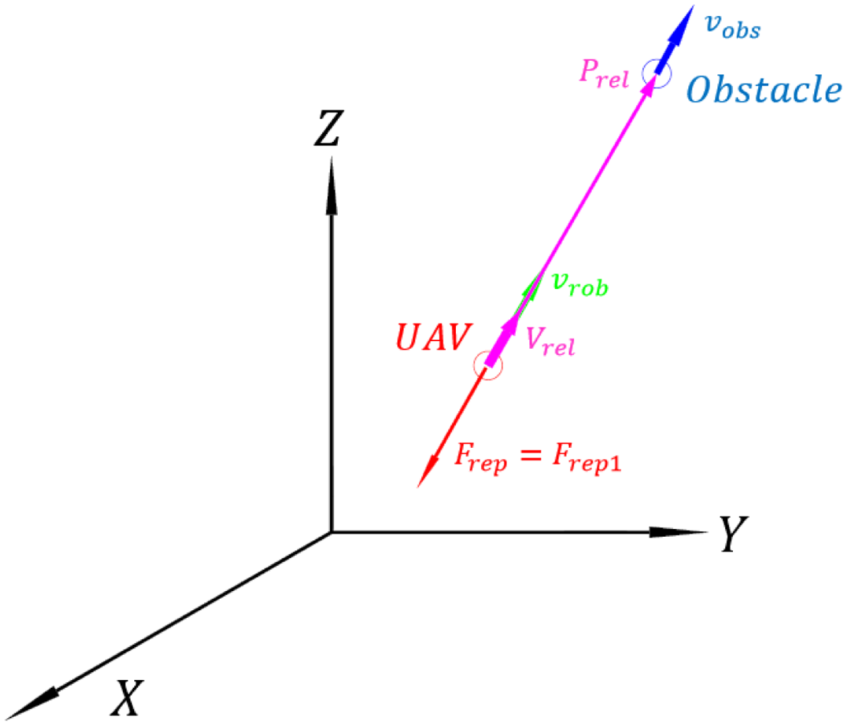
The LMP occurs in the 3D environment when UAV, obstacle, or resultant forces from all obstacles and the target are acting on the same line of action. At the beginning of this situation, the UAV is influenced by the attractive force and thus causes the UAV to move toward the target until it enters the IR of the obstacle. Under this circumstance, the UAV is influenced by the target and the obstacle where the attractive and repulsive forces are affecting the UAV. The attractive force and repulsive force are in the same line, but each one is opposing the other. This causes the UAV to reduce its velocity until both forces are equal. As a result, the UAV stops its motion waiting for the obstacle or target to change its location, so the three objects are not on the same line of action, as shown in Fig. 16. Another situation resulted when both target and obstacle moved in constant velocity and on the same line of action, as shown in Fig. 17. When this problem happens, the repulsive force has only one term, which is
 $ F_{\textrm{rep}1}$
, the second term of the repulsive force which is
 $ F_{\textrm{rep}2}$
, approaches zero. This is because the relative velocity vector between the UAV and the obstacle is in the same direction as the relative position vector between the UAV and the obstacle. Figure 18 shows complete demonstration of this situation. When the UAV, the obstacle, and the target on the same line of action, the relative velocity vector and the relative position vector between UAV and target are in the same direction. In this case,
 $\mathcal{L}_x=\zeta _x$
,
 $\mathcal{L}_y=\zeta _y$
, and
 $\mathcal{L}_z=\zeta _z$
. Furthermore, the attractive force acts in the opposite direction of
 $ F_{\textrm{rep}1}$
so
 $\varepsilon _x=\pi -\zeta _x$
,
 $\varepsilon _y=\pi -\zeta _y$
, and
 $\varepsilon _z=\pi -\zeta _z$
. After drawing the free body diagram for the UAV in LMP situation and assuming that UAV is
 $ 1 \ \textrm{kg}$
mass, the acceleration of the UAV in the LMP is presented in the following equation:
 \begin{equation} \left [ \begin{array}{c} \ddot{x} \\ \ddot{y} \\ \ddot{z} \\ \end{array} \right ]=m\alpha _p\parallel P_r\parallel{}^{m-1}\left [ \begin{array}{c} \cos \left (\zeta _x\right ) \\ \cos \left (\zeta _y\right ) \\ \cos \left (\zeta _z\right ) \\ \end{array} \right ]+n\alpha _v\parallel V_r\parallel{}^{n-1}\left [ \begin{array}{c} \cos \left (\zeta _x\right ) \\ \cos \left (\zeta _y\right ) \\ \cos \left (\zeta _z\right ) \\ \end{array} \right ]+\parallel F_{\textrm{rep}1}\parallel \left [ \begin{array}{c} \cos \left (\pi -\zeta _x\right ) \\ \cos \left (\pi -\zeta _y\right ) \\ \cos \left (\pi -\zeta _z\right ) \\ \end{array} \right ] \end{equation}
To overcome these issues, the resultant forces is augmented with an additional term to detect the trap position when the total force is equal to zero. Then the UAV has the ability to maneuver by applying the augmented force term to the UAV and escape from the trap position due to LMP. The augmented additional term has the same magnitude of the repulsive force but acts on another corrected direction at the trap position, as follows:
 \begin{equation} \overrightarrow{F}_{\textrm{total}}=\overrightarrow{F}_{\textrm{att}} + \overrightarrow{f'}_{\textrm{rep}1} \end{equation}
 \begin{equation} \overrightarrow{f'}_{\textrm{rep}_1}=\overrightarrow{f}_{\textrm{rep}_1} + \delta \left (\left \| \overrightarrow{F}_{\textrm{att}} + \overrightarrow{f}_{\textrm{rep}1} \right \|\right )\begin{bmatrix} \textrm{Cos} (\mu ) & - \textrm{Sin}(\mu ))& 0\\ \textrm{Sin}(\mu ) & \textrm{Cos}(\mu )& 0\\ 0& 0 & 1 \end{bmatrix}\begin{bmatrix} f_{\textrm{rep}1x}\\ f_{\textrm{rep}1y} \\ f_{\textrm{rep}1z}\\ \end{bmatrix} \end{equation}
where
 $\delta (\tau )= \left \{\begin{matrix} 1 &, \tau =0\\ 0 &, \tau \neq 0 \end{matrix}\right .$
. And
 $ \mu = \sin ^{-1}(||f_{\textrm{rep}1}||/||F_{\textrm{att}}||)$
, at the local minimum condition
 $\mu = \pi/2$
and the repulsive force is
 \begin{equation} \overrightarrow{f'}_{\textrm{rep}1}= \overrightarrow{f}_{\textrm{rep}1} + \begin{bmatrix} 0 & -1 &0 \\ 1& 0 & 0\\ 0& 0 & 1 \end{bmatrix} \begin{bmatrix} f_{\textrm{rep}1x}\\ f_{\textrm{rep}1y}\\ f_{\textrm{rep}1z} \end{bmatrix} \end{equation}
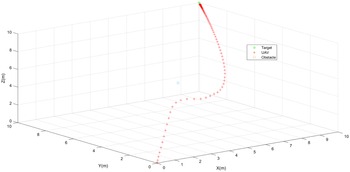
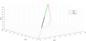
The proposed solution successfully solves the LMP for stationary and moving objects, see Figs. 19 and 20.
4. Performance analysis of the proposed algorithm
In order to check the performance of the proposed algorithm with the increasing number of obstacles, a statistical study is carried out for
 $125$
simulations. In each simulation, the UAV starts its movement form
 $ [0\; 0\; 0]^T$
with zero initial velocity where the target is stationary at
 $[5\; 5\; 5]^T$
. So the operating space is
 $ [5 \times 5 \times 5]^T \textrm{m}^3$
. Furthermore, the IR of the obstacle is selected to be 1.5 m and the repulsive force is multiplied by a scaling parameter
 $\eta =0.3$
.
The IR and
 $\eta$
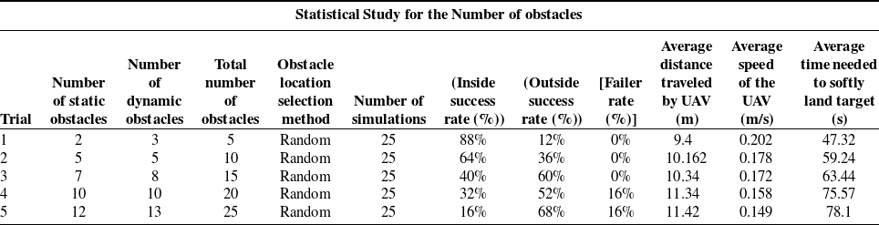
are related to each other. In the first trial, five obstacles were used, three of which were dynamic obstacles and the location of each obstacle was selected randomly to be in the first quarter. A number of 25 simulations are performed; and in each simulation, the UAV successfully softly lands on the target after 47.32 s without colliding with any of the five obstacles. Moreover, in this trial, the UAV traveled with an average path of 9.4 m during the average time of 47.32 s. Other trials are detailed in Table II.
We can conclude from the table that by increasing the number of obstacle in the space, the inside success rate (the UAV successfully softly lands on the target without going outside the
 $[5\times 5 \times 5] \ \textrm{m}^3$
operating space) is decreased dramatically from
 $88 \%$
in the first trial to
 $16\%$
in the last trial. However, the outside success rate is increased from
 $12\%$
in the first trial to
 $68\%$
in the last trial. Moreover, the failure rate (the UAV did not softly lands on the target) increased from
 $0\%$
in the first trial to
 $16\%$
in the last trial. On the other hand, by increasing the number of the obstacles, the total distance traveled by UAV increases because the UAV maneuvers more in the space to avoid the increasing number of obstacles and requires more time to softly lands on the target. So the average speed is also decreased by increasing the number of obstacles. While the time needed by the UAV to softly lands on the moving target increases. The detailed distances, speeds, and time for the UAV in the 125 simulation are plotted in Figs. 21−23.
Time history of the three vehicles trajectories.

Experiment snapshots taken during one of the tests that show the position of the vehicles during the maneuver.

5. Experimental results
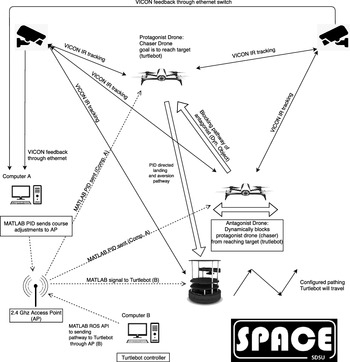
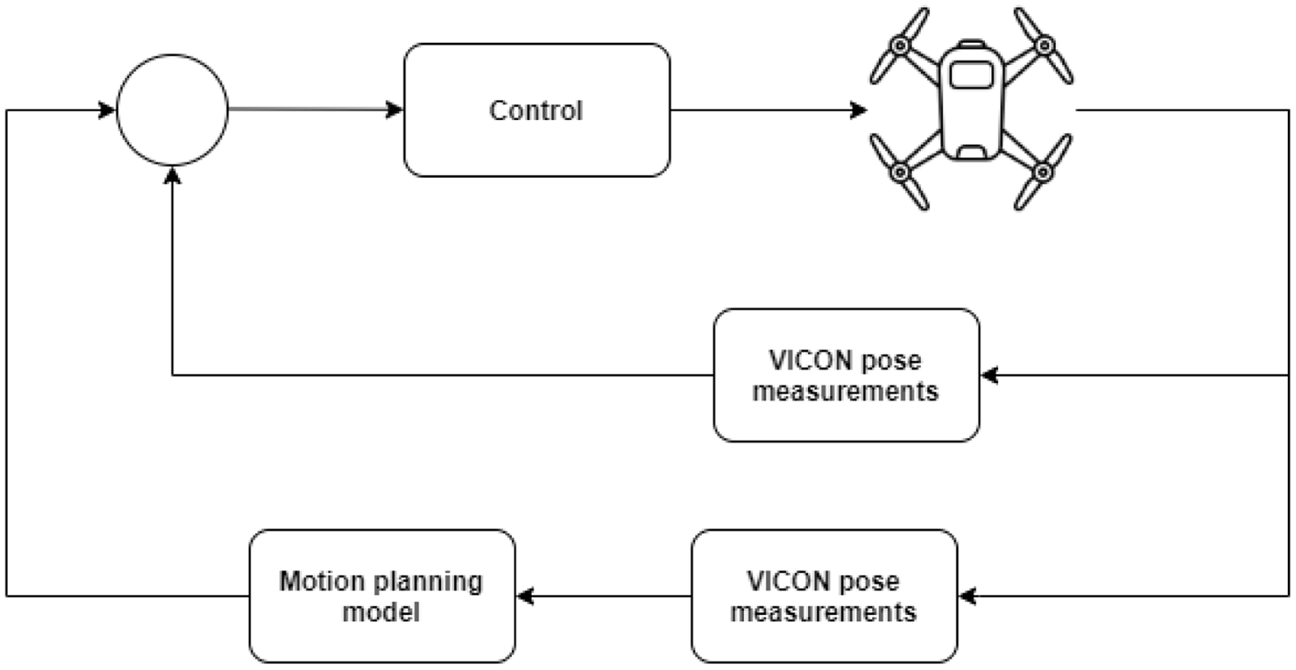
In this section, an experiment is conducted in the Spacecraft Platform of Astronautics and Celestial Emulation (SPACE) laboratory to simulate the path planning of an UAV in a 3D dynamic environment. The SPACE laboratory is fully equipped with a guidance, navigation, control (GNC) platform to emulate six degrees of freedom vehicle motion in submillimeters resolution. Figure 24 shows the hardware and platform setup of the experiment. Three platforms are used: two parrot bebop drones, one is a chaser (protagonist) and one is a dynamic obstacle (antagonist), and a Turtlebot robot as a landing target. Six 16MP-VICON cameras are utilized to measure the pose information of the three platforms. The pose rates are estimated using the VICON measurements. The chasing drone receives GNC commands to follow the planned motion given in the generalized potential force functions. As shown in Fig. 24, the Turtlebot robot (target) moves in configurable paths controlled by Computer B via MATLAB ROS API. Both the protagonist and antagonist drones are commanded through Computer A. The antagonist drone flies according to random trajectories around the target (Turtlebot) to block the protagonist drone from reaching a safe land on the target (Turtlebot). All three platforms are controlled using PID control laws to follow the desired paths. The PID controllers receive the pose information for each platform from the VICON system and compute the necessary commands, so each platform follows its desired path. Figure 25 shows the feedback control implemented to pilot the protagonist drone safely through the antagonist environment and land on the target (Turtlebot). Both the Turtlebot and the antagonist drone have predetermined paths. The motion planning model computes the desired 3D waypoints for the protagonist drone using the generalized potential force functions based on the measured position information of the three vehicles from the VICON system. The protagonist drone has an onboard PID controller that takes the VICON measurement to compute the error departure from the desired waypoints and commands the drone to follow the waypoints.
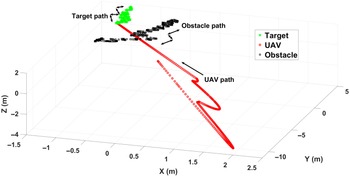
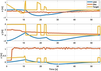
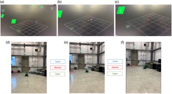
Figure 26 exhibits the 3D trajectories for the three platforms simulated in the SPACE laboratory. Several tests have been conducted to ensure the robust and efficient maneuver of the protagonist drone by tuning the onboard control system. Also, Fig. 27 shows the time history of the three vehicle trajectories during the experiment. Figure 28 exhibits snapshots of the three vehicles taken during one of the experiments. The target vehicle is labeled in the green box, the obstacle vehicle in the red box, and the chaser vehicle is a blue box. In Fig. 28, the positions of the three vehicles are displayed just after take-off (a) and (d), during maneuver (b) and (e), at landing (c) and (f). Figure 28(a−c) are shown in VICON tracker.
6. Conclusion
In this research, the motion planning system in 3D dynamic space is implemented for UAVs operation. The system provides a systematic approach to extend the generalized potential field forces to be used in a 3D dynamic environment for UAV motion planning. In this system, the UAV is considered to be moving under the influence of attractive and repulsive forces in 3D space simultaneously. Most of the implemented approaches tried to treat the motion planning problem in 3D as a projection in 2D space at a given altitude with fixed obstacles. The quadrotor in this paper is considered to be moving under the influence of attractive and repulsive forces in the 3D space simultaneously. As a result, the quadrotor changes its altitude and projected planner position concurrently when both target and obstacles are dynamic. The presented analytical implementation provides the reader with a systematic approach to implement and validate the APF in 3D dynamic environments. Moreover, LMP in 3D static and dynamic environments is analyzed and resolved. Simulations, as well as experiments, are conducted to validate the systems for UAVs operation in a 3D dynamic environment. An optical tracking system is used to provide the pose information of the moving objects during real-time runs using six Vicon cameras. The demonstrated results show the effectiveness of the motion planning system, and the LMP was successfully solved for stationary and moving objects.
Ethical approval
This article does not contain any studies with human participants or animals performed by any of the authors.
Authors contributions
All authors contributed equally.
Funding
This research received no external funding.
Competing interests
The authors declare that they have no conflict of interest.
Availability of data and materials
The data that support the findings of this study are available from the corresponding author upon reasonable request.