1. Introduction
Many developing countries obtain a large share of their income from the harvesting of common property or open access renewable natural resources, including fisheries, forests, grazing grounds, and water resources. The literature, which originated in Scott Gordon's (Reference Gordon1954) classical paper, has emphasized the effect of these activities on the renewable natural resources which in turn are a key factor of production. The issue is that these harvesting activities are not only resource-impacting but, most importantly, also highly resource-dependent. When the number of producers using open access resources is large, there is overexploitation and excessive degradation of such resources that in the end makes producers poorer (the so-called ‘tragedy of the commons’).
However, as this literature emphasizes, even in the complete open access case there are automatic mechanisms that place limits to the extent of resource degradation. The main reason for this is the high dependence of harvesting on the renewable resources; as the natural resource deteriorates, productivity of the harvesting effort falls which in turn reduces the incentives to spend efforts in the harvesting of such resource. In the end there may be a long-run equilibrium in which the level of harvesting of the resource is equal to the regeneration of the renewable resource and the value of the average product of effort in exploiting the resource is equal to the (opportunity) cost of such effort in alternative activities. At this point no further deterioration of the resource or of the income of the producers occurs. To emphasize the importance of the feedback productivity effects associated with the degradation of renewable resources as a stabilizing mechanism, we call these activities ‘resource-dependent’ sectors (or, at times, simply ‘harvesting’ sectors).
The automatic resource stabilizing effect as considered in the standard literature implicitly assumes that the alternative activities that dictate the opportunity cost of harvesting effort do not rely on the renewable natural resource as a factor of production. Moreover, it must also be the case that in the standard model the nonharvest production activities are not resource-impacting either. In reality, however, many of the most important alternative production activities, especially in developing countries, while not dependent on the renewable resources as a factor of production, do impact on them. Most industrial production as well as the extraction of exhaustible resources and energy production impact upon the renewable natural resources despite the fact that the renewable resource is not a factor of production for these activities.Footnote 1 Mining, coal extraction, hydroelectric power generation, various manufacturing activities as well as oil and gas extraction severely impact on the renewable resources, often affecting water supplies, causing water and soil contamination, flooding of large areas sometimes formerly used by small producers, deforestation, degradation of fisheries, and more. Henceforth, we call these industries ‘resource-impacting’ sectors (or at times simply ‘industrial’ sectors).
Since the resource-impacting sectors do not use the renewable resource as a factor of production, the automatic equilibrating mechanism prevailing in the standard case of resource degradation by harvesters of such resources is in principle absent for resource-impacting activities. The degradation of the renewable resource may not discourage the expansion of the resource-impacting activities. So even if there were a third sector that was neither resource-dependent nor impacting, there is no inherent mechanism that would limit production-induced damages upon the renewable resources caused by these sectors. Thus, the potential environmental destruction and consequent impoverishment of the resource harvesters could be much more serious in this case compared to the standard one. In the absence of regulation mitigating the impact effect of the resource-impacting sectors on the renewable resources, the extent of the resource destruction could be completely unchecked. However, using a formal model we show below that the above intuition is not always right, but we ascertain the specific conditions required for it to be, in fact, correct.
Another significant difference between resource-dependent and resource-impacting activities is that the former tend to involve very large numbers of mostly self-employed and poor producers relying mainly on labor-intensive technologies, while the latter are comprised of relatively few large firms that tend to be capital intensive. This is an important issue that the ensuing theoretical model highlights.
In general most resources of great economic importance are inherently open access. The fact that the resource-dependent sector is composed of so many small producers renders it almost impossible to regulate them. Also, as Partha Dasgupta has often emphasized, the fact that most natural resources such as animals, insects, rivers, ground water, fish resources and the atmosphere are frequently mobile renders it almost impossible to establish or enforce property rights (Dasgupta, Reference Dasgupta, Simpson, Toman and Ayres2005).Footnote 2 The idea of setting property rights on these resources is a chimera and so is that concerning ‘optimal’ taxes or regulations that could have a chance of effective enforcement.
By contrast, the fact that the resource-impacting sector is often comprised of few and large firms using capital-intensive technologies, would in principle facilitate regulating them, for example, as some countries try to do, by requiring environmental impact assessments as requisites to approving capital investment projects. Paradoxically, however, the very fact that these firms are large makes them economically and politically powerful which itself becomes an obstacle for their effective regulation. This is true for developing countries and even for a country as advanced as the USA as none other than President Obama has recently recognized in connection with the oil disaster in the Gulf of Mexico: ‘For too long . . . there has been a cozy relationship between the industry and the [regulators] that permit them to drill . . .’ (Tumulty and Eilperin, Reference Tumulty and Eilperin2010). Similar remarks have often been made concerning other major disasters caused by other resource-impacting industries including coal mining. The regulators often sleep with the regulated. For these reasons we make no apologies for the assumption of open resource access made throughout the theoretical model.Footnote 3
There is increasing empirical evidence regarding the importance of the nonharvesting yet renewable resource-impacting activities as a source of destruction of such resources (Engel and López, Reference Engel and López2008). Documented cases include oil and gas extraction in the Amazon, Indonesia, and sub-Saharan Africa affecting forest and water resources and impairing the livelihood of local communities; mining in the arid deserts of Chile (mineral extraction and processing being highly intensive in the most scarce renewable resource, water) resulting in ground water depletion hurting hundreds of thousands of indigenous people that have been forced to migrate; oil and gas exploration in forests of Ecuador hurting renewable resource-dependent local communities for many years; gold extraction in the north of Chile and Argentina threatening a large glacier which is a vital source of irrigation and drinking water; coal extraction especially using mountain top removal which causes large negative impacts on forests and water resources.Footnote 4
The impacts of oil spills on marine and other renewable natural resources are by now legendary. According to reports, every year on average oil extraction in Nigeria causes one disaster as large as the Exxon Valdéz was (Nwilo and Badejo, Reference Nwilo, Badejo, Sutherland and Nichols2006). Some 230,000 cubic meters of oil – from at least 300 spills – contaminate the Niger delta region annually (Moffat and Linden, Reference Moffat and Linden1995). In Mexico, unregulated oil extraction has forced massive relocations and led to hazardous living conditions including the release of toxic substances and disruption of water supplies damaging crops and depleting fish populations (Chelala, Reference Chelala1998). In Ecuador, extremely high levels of water pollution affecting the livelihood of hundreds of thousands of people depending on harvesting activities have been attributed to contamination from unlined waste pits created by Texaco's involvement in the Ecuadorian forests (Kane, Reference Kane1996; Brooke, Reference Brooke1994).Footnote 5
Despite the empirical importance and potential conceptual ramifications of the existence of resource-impacting industrial or extractive sectors on the renewable resources and on the income of often poor harvesters, the modeling efforts have mostly ignored the interactions between resource-dependent and resource-impacting sectors. Some authors look at the management of the commons by harvesters mostly in isolation from the rest of the economy and concentrate on factors that affect the management efficiency of the commons (Ostrom, Reference Ostrom1990; Ostrom et al., Reference Ostrom, Gardner and James1994; Baland and Platteau, Reference Baland and Platteau1997, Reference Baland and Platteau1998). Other studies do consider general equilibrium interactions of the harvester sector with the ‘rest of the economy’, but have often used models based on Brander and Taylor (Reference Brander and Taylor1997), where the alternative sectors are ‘clean’, i.e., they do not impact the resource stock (Brander and Taylor, Reference Brander and Taylor1998; Copeland and Taylor, Reference Copeland and Taylor2009; and many others).Footnote 6
While these analyses examine the dynamics of the renewable resource, they are static in all other respects by not allowing for capital investment and for the interactions between capital accumulation and the renewable resource dynamics. That is, they are not suitable to analyze sustainable economic development. In this literature the ‘other’ sector (in our case the resource-impacting sector) is static and its only role is competing for labor with the resource-dependent sector thus dictating a fixed opportunity cost to the harvesters. By contrast, in our analysis the ‘rest of the economy’ plays a much more fundamental role having its own endogenous dynamics, in turn triggered by the incentives to save and capital accumulation arising from market conditions. This endogenous dynamics plays a vital role as a source of economic development and in determining the sustainability characteristics of such development. Our focus is on characterizing the process of economic development rather than on static trade patterns as most of this literature does.
The mechanics of the ensuing model is as follows: the industrial resource-impacting sectors recruit their work force from the large number of harvesters and invest in physical capital. The expansion of the industrial sector directly impacts on the renewable resource causing its degradation. This in turn may reduce the productivity of harvesters and in principle make it possible for the industrial sector to pay lower wages. On the other hand, the fact that the industrial sector pulls labor out of the harvesting sector has the opposite effect on the natural resource by decreasing harvesting pressures. A third aspect to consider in the analysis is the fact that the expansion of the industrial sector also causes the price of the harvested good to increase in a closed economy or in an open economy able to influence world prices. The price effect makes recruitment of harvesters a bit more expensive to the industrial firms and at least partly mitigates the possible income losses that harvesters could suffer as a consequence of the degradation of the natural resource.
2. The production sectors
We consider two production sectors, a renewable resource-dependent or harvesting sector and the resource-impacting or industrial sector. The natural resource is under open access regime. To emphasize the differences in capital intensity between the two sectors we assume that the resource-dependent sector uses only labor and the natural resource as factors of production, while production of the resource-impacting sector uses both labor and capital. We assume that harvesting of the renewable resource is carried out according to the standard production function originally proposed by Schaefer (Reference Schaefer1957) and subsequently used by many other authors (i.e., Copeland and Taylor, Reference Copeland and Taylor2009; Brander and Taylor, Reference Brander and Taylor1998; Clark, Reference Clark1990, and many others),

where N is the stock of natural resource, LE is the level of employment in the sector, and A is a fixed productivity factor.
The resource-impacting sector is capital intensive so its production uses capital in addition to labor. We assume a Leontief production function for this sector,Footnote 7
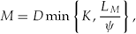
where M is output level, K is the stock of capital used by the resource-impacting sector, LM is labor, D is a productivity parameter, and ψ is the labor-to-output ratio. Given that we have normalized the capital-output ratio to one (one over D indeed), ψ is also the labor to capital ratio. That is,


The total labor endowment of the economy is fixed at L so that the employment level in the resource sector is LE = L − LM. The resource-dependent sector picks up whatever labor is not employed by the industrial sector. Using (3ii) we have that

The natural resource stock is subject to the following dynamics:

where N is the stock of renewable resources, g(N) is a function representing the natural renewal of the resource, and the parameter φ represents the resource impact factor of the industrial sector production. The most important difference between this formulation and the standard one is that (5) allows for the industrial sector to impact on the renewable natural resource stock, despite the fact that its production does not depend on it.
We specify the standard logistic model for natural resource renewal function, g(N) = rN(1 − N/ ), where r is the intrinsic growth rate of the natural resource and is the maximum carrying capacity of the natural system (Clark, Reference Clark1990). Using (1), (3), and (4) in (5), we obtain an explicit representation of the resource dynamics

3. The consumption sector
We assume that the representative consumer has the following indirect utility function:

where  is the total nominal consumption expenditure, p 1 and p 2 are the prices of the industrial good and resource good, respectively, and e(p 1, p 2) is the (indirect) unit expenditure function or cost-of-living index (so that /e(p 1, p 2) is the real level of consumption). Preferences are assumed to be Cobb–Douglas which means that the unit expenditure function is also Cobb–Douglas

where β is the fixed expenditure share of the industrial good and 1 − β is the share of the resource good in the consumer budget.
Using Roy's identity we can derive the consumer demands for the two goods
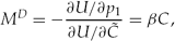

In (9) and (10) we have normalized by the price of the industrial good so that C ≡ /p 1 is the total consumption expenditure in units of the industrial good and p ≡ p 2/p 1 is the relative price of the resource good.
4. Market equilibrium conditions
Since the two sectors compete for labor we have that both sectors have to pay the competitive wage rate. If H > 0, then the economy's wage rate is equal to the average value product of labor in the harvesting sector. Given that a closed economy remains diversified, H > 0, which implies that the wage rate in units of the industrial good (w) is

The market clearing condition for the resource-dependent or harvested good requires that

The industrial good is assumed to provide the material goods for new capital investments as well as for consumer goods. Hence, production of the resource-impacting or industrial good must be equal to the consumer demand for the good plus the capital investment. Thus, using (3i) and (9), we have

where I is gross investment in new capital.
Finally, the demand for investment goods is assumed to be proportional to the level of profits in the industrial sector, where profits π = DK − wLM. Thus we have

where 1 > s > 0 is a fixed parameter that can be interpreted as the rate of savings out of profits. That is, we are assuming that the economy is poor so that workers, whether in the resource-dependent or in the resource-impacting sector, do not save. Only capitalists save part of their profits.Footnote 8
Equilibrium in the industrial good sector implies that I = ID which, using (13) and (14), imply that

Finally, the change of the stock of capital over time is

where δ is the fixed rate of depreciation of the stock of capital.
5. Solving the temporary equilibrium
The equilibrium conditions (11)–(15) in conjunction with the labor market equilibrium condition given by (4) solve for the temporary equilibrium values of the six endogenous variables, w, C, p, LE, LM, I. This is a temporary equilibrium solution in the sense that the solution values are all conditional on the initial levels of the stocks of capital and natural resources, K and N. The subsequent dynamics of these stocks in turn is determined by the temporary equilibrium values of the above-mentioned endogenous variables.
Using (11) and (12) in (13), we obtain
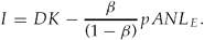
Combining (4), (14) and (17) we solve for the equilibrium level of the wage rate, pAN,

Thus, as expected, the equilibrium level of the wage rate is increasing in K and decreasing in the size of the labor force, L. Significantly, the harvesters’ income per unit of effort is not dependent on the stock of natural resources. A positive equilibrium wage rate requires that the denominator in (18) be positive. Then we have the following lemma.
Lemma 1. The level of pAN > 0 if and only if K < βL/[(β + (1 − β)s)ψ].
This lemma implies that the resource-dependent sector can survive (by paying a positive per capita income to the harvesters) only if the stock of capital in the industrial sector is not too large relative to the total labor force. In general the wage rate is increasing in K. As long as K is below the limit indicated in Lemma 1, pAN can be equal to the wage rate as indicated by (11), but if K is above that limit the average income in the harvesting sector cannot match w anymore and hence (11) would become an inequality with w > pAN; in this case all harvesters would move to the industrial sector and the resource sector would not be able to survive. However, below Lemma 2 shows that the long-run equilibrium level of K is in fact lower than the limit established in Lemma 1 for w = pAN > 0.
The following proposition follows if the condition of Lemma 1 holds:
Proposition 1. Assume that the condition in Lemma 1 is satisfied (i.e., the economy is diversified) then the per capita income of workers engaged in harvesting activities is increasing in K regardless of the impact of K on the stock of natural resources.
Proposition 1 can be shown by inspection of equilibrium condition (18). The per capita income of the harvesters (pAN) is increasing in K. Even if the expansion of the industrial sector associated with a higher level of K causes the natural resources to contract, the income of the harvesters increases. The reason for this is that any fall in N that a higher K might trigger would be compensated by a more than proportional rise of the price of the harvested good. What happens is that the increase in K has both a cost push and a demand effect that magnify the impact on p.
Finally we use (3i), (3ii), (11), and (18), and the definition of profits provided above (π = DK − wLM) to obtain the equilibrium level of profits

6. The dynamics of the stock of capital
Using (14), (16), and (18) (recalling that w = pAN), we obtain the capital accumulation equation

or, equivalently, the rate of capital accumulation,  ≡
 /K, is

Equations (20) or (20i) characterize the dynamics of the capital stock. From (20i) it follows that there is a unique long-run equilibrium level of K at which = 0

where ξ ≡ (sD − δ)/sψ. In (21) the long-run equilibrium level K* is positive if ξ > 0, which in turn means that D − δ > 0; that is, if the rate of savings per unit of capital is greater than the rate of depreciation of capital that is indeed a necessary condition for the economy to be able to invest at all.
Also, there is an absolute maximum feasible value for K defined by the total labor endowment of the economy. Suppose that K is so large that all the labor force gets absorbed by the industrial sector. Then we have that the maximum level of capital is Kmax = L/ψ. The economy would not invest beyond this level. From (21) it follows that indeed K* < Kmax. In addition, comparing the condition for pAN > 0 established in Lemma 1 and (21) it is clear that

Hence we have the following lemma.
Lemma 2. (a) The long-run equilibrium level of the stock of capital satisfies the condition of Lemma 1 and therefore pAN > 0. Thus an economy that is initially diversified (i.e., that initially produces both final goods) remains diversified into long-run equilibrium. (b) This also implies that the absolute maximum constraint for K(Kmax) is never binding, that is, K* < L/ψ.
Thus, Lemma 2 shows that diversification as required by the fact that the closed economy must consume both goods is in fact consistent with the long-run equilibrium level of capital. Moreover, as long as the economy initially produces the resource commodity it can continue doing so indefinitely.
Moreover, from (20) it is easy to see that > 0 if K < K* and < 0 if K > K*. That is, the dynamics of the capital stock is quite straightforward: there is a unique level of K at which capital becomes constant and the stock of capital globally converges to such equilibrium level. We now turn to the characterization of the dynamics of the stock of natural resources.
7. The dynamics of the natural resource
Long-run equilibrium in the resource sector implies that  = 0. Hence, using (6), we have

Define the following variable:
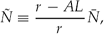
which could be interpreted as the hypothetical level of N that would prevail in the long run if K = 0. We note that Ñ > 0 as long as production of the harvest good is feasible over the long run. In fact, it can be easily seen from (22) that r − AL is the slope of the = 0 schedule when N = 0, which has to be positive. Then we can rewrite (22) as follows:

Thus using (24) it follows that two cases are possible:
(i) Assume that ψ AÑ < φ D then N ≥ Ñ is not compatible with a positive level of K/N. Hence, it must be the case that along the
 = 0 schedule, N < Ñ. Thus, in this case we have that ψAN < φD for all feasible levels of N under the assumption ψ AÑ < φ D. Also, as we show below, in this case the = 0 schedule has a segment that is downward sloping and another one that is upward sloping.
(ii) Assume that ψ AÑ > φ D then the
= 0 schedule is consistent with K/N > 0 only if N > Ñ. This means that ψAN > φD for all feasible levels of N in this case. Now, the = 0 schedule is upward sloping for all levels of K and N ≤ .
Below we characterize the = 0 schedule for each case. Also, from (24) it follows that along the = 0 schedule we have that
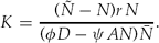
The economic meaning of all this can be made clear by the following experiment: suppose that initially K = ϵ, where ϵ is an arbitrary small number as close to zero as possible (but not quite zero because in a closed economy we need a positive level of both outputs). Then Ñ is an approximation to the equilibrium level of N that would prevail if the industrial sector is minimal and almost all the labor force is employed in the resource-dependent or harvesting sector. The term φ D − ψ AÑ represents the net marginal effect of expanding the industrial sector (i.e., of increasing K) on the natural resource degradation at this point. It is comprised of the direct impact effect (φD) which is always positive (that is, it always increases resource degradation) and the indirect impact (–ψAN) caused by the fact that an expansion of the industrial sector induces a reduction in the level of employment in the harvesting sector which in turn reduces pressure on the natural resource. Cases (i) and (ii) above represent the cases when the net impact of K on the degradation of N is negative and positive, respectively. So in case (i) capital accumulation starting when N ≈ Ñ causes N to fall, while the opposite happens in case (ii).
8. Development paths
Before we proceed to characterize the development paths of the economy under each of the above cases, we need to define our concept of sustainable development.
Definition. An economy is said to be sustainable if it follows a path that converges toward a steady-state equilibrium characterized by a positive and stable level of the natural resource. More formally, a sustainable development path implies that limt → ∞N(t) ≡ N* > 0.
Note from the above definition that in contrast with sustainable development, unsustainable development would be characterized by a path where N continuously declines along the growth process but does not become zero in finite time as long as the economy is closed. We now characterize the development patterns of the economy when cases (i) or (ii) prevail.
Case (i): the net impact of the industrial sector is to increase resource pressure (ψ AÑ < φ D)
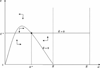
In this case the marginal impact on the natural resource of industrial workers (equal to φD) is greater than the maximum marginal impact of harvesters (equal to ψ AÑ). We note that ψ AÑ is the maximum impact because as we showed above, in case (i) we have that N ≤ Ñ. In this case the = 0 schedule as shown in (25) must lie completely to the left of Ñ for positive levels of K (figures 1a and 1b); that is, the = 0 schedule is defined only for N ≤ Ñ.
Case i: Aψ Ñ < φ D with sustainable long-run equilibrium

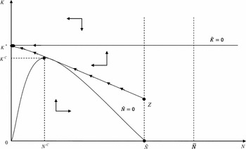
Case i: Aψ Ñ < φ D with unsustainable long-run equilibrium

From (25) it follows that along the = 0 schedule we have that K = 0 if either N = Ñ or N = 0. Also, the slope of the = 0 curve is negative when evaluated at N = Ñ and it is positive when evaluated at N = 0. Finally, as we show below, the = 0 curve reaches a maximum at a unique level of N, which means that this curve has an inverted U shape. The = 0 curve in figures 1a and 1b is drawn consistent with this characterization.
Figure 1a shows the case when sustainable development is possible. This is the case when K* is below the maximum height of the = 0 curve as happens in Figure 1a. The long-run equilibrium of the system is shown in Figure 1a by the coordinates labeled N* and K* which simultaneously satisfy the conditions = 0 and = 0. In Figure 1a there is another lower level of N that also satisfies this condition, but it can be easily seen that such equilibrium is unstable.
The arrows show the motion of the system outside the steady state. As can be seen in Figure 1a, for levels of K above those required by the = 0 condition, the stock of the resource declines and it increases for levels of K below the = 0 curve. This can be seen by inspecting (22) and is due to the fact that in this case ψ AÑ < φ D. Also, as discussed in the previous section, the dynamics of the stock of capital as shown by (20) implies that K increases (decreases) if K < K* (K > K*) regardless of the level of N. Thus, the = 0 schedule is a horizontal line in the K − N space as drawn in the figures.
We now turn to determine the maximum height of the = 0 curve. Differentiating (25) and making the derivative expression equal to zero, we find that the critical level of N at which this curve reaches its maximum height is
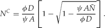
We note that the solution is real because case (i) implies that ψ AÑ/φ D < 1. Also, consistent with this case we have chosen the negative root solution because NC < Ñ < φD/ψA. The maximum level of K consistent with the = 0 condition is obtained by using (26) in (25):
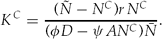
The key issue is whether K*as defined by (21) is above or below KC. If K* < KC as in Figure 1a, sustainable development is possible; however, if K* > KC, then sustainable development is not possible; that is, in this case limt → ∞N(t) = 0. The level of the resource continuously falls (and p continuously increases) over time. By solving (22) it can be shown that N* > 0 if K* < (r − AL)/ψA. This condition is in fact equivalent to the condition K* < KC.
Figure 1b shows the case where K* > KC (or equivalently, K* > (r − AL)/ψA). Now, unlike the case drawn in Figure 1a, the system cannot achieve sustainable equilibrium over the long run. The arrow line Z K* represents a possible (unsustainable) pathway for an economy that starts with a low level of capital and a relatively high endowment of N and converges toward resource extinction, but never quite reaches that level in finite time.
The following proposition emerges from the previous analysis.
Proposition 2. Assume that ψ AÑ < φ D. Then the expansion of the industrial or resource-impacting sector necessarily reduces the stock of natural resources. Industrial expansion may in this case even threaten sustainable development. The likelihood of unsustainable development is increasing with the economy's saving rate (s), with the share of the industrial good in the consumer budget (β), and with the gross or direct resource impact effect of K (φD), and decreasing in ψA. Also, the population size (L) increases the risks of unsustainable development.
All results in Proposition 2 follow directly by comparing (21) and (27) using (26) with the aid of figures 1a and 1b. The results in Proposition 2 make intuitive sense. Under the condition of case (i), the industrial sector is more resource demanding than the harvest sector. Hence industrialization necessarily reduces the stocks of natural resources. The second part of Proposition 2 describes the conditions under which the effect of industrialization goes beyond merely the reduction of the stock of natural resources and threatens sustainable development.
An economy that expands capital fast (i.e., an economy that has a high level of savings) and where consumers’ demand for industrial goods is large is more likely to follow an unsustainable development path than an economy where consumer and investment demand for the industrial good are low. Also, the risk of unsustainable development increases the greater is the difference of the marginal destructive effects on the natural resource between workers employed in the industrial sector and those in the harvest sector (φD − ψ AN). Finally, a larger size of the labor force allows a greater expansion of the industrial sector that causes a greater negative impact upon the natural resource. Increasing L raises the steady-state level of capital, K*, and reduces the maximum level of K that is compatible with sustainable development, Kc.
Several of the factors that increase the likelihood that industrialization will trigger unsustainable development shown by Proposition 2 are often present in developing countries. For example, fast industrializing China and India have extremely high savings rates, very large populations and consumers have a high preference for industrial goods as reflected in large budget shares for such goods.
The following proposition characterizing the long-run equilibrium for case (i) follows from the previous analysis.
Proposition 3. Assume that ψ AÑ < φ D. Then when K is in long-run equilibrium (i.e., K = K*), we have that K, C, LE, and pAN are all constant. If K* < KC, then in long-run equilibrium = 0 and thus the constancy of the wage rate, pAN, is achieved at constant levels of both N and p. However, if K* > KC, then in long-run equilibrium < 0 and hence the constancy of pAN requires that  /p = − /N > 0.
Proposition 3 follows from the fact that when K becomes constant equal to K* we have that by (4) LE is constant and by (18) pAN is also constant. Also by (12) total consumption expenditures, C, are also constant in the long run. In addition, a constant level of pAN can be achieved by a constant level of both p and N, which corresponds to the case of sustainable development depicted in Figure 1a or, alternatively, by N falling and p increasing proportionally to the fall in N. The latter is of course the case of unsustainable development that occurs when K* > Kc as depicted in figure 1b.
Case (ii): the net impact of the industrial sector is to reduce resource pressure (ψ AÑ > φ D)
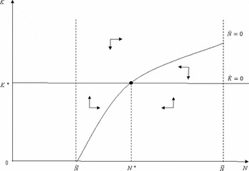
In this case the marginal impact of industrial workers on the natural resource (equal to φD) is less than the minimum marginal impact of harvesters (equal to ψ AÑ). Evaluating N at Ñ yields the minimum impact of harvesters in case (ii) because now N ≥ Ñ. Figure 2 depicts this case. The = 0 schedule is now upward sloping for Ñ ≤ N ≤ .Footnote 9 Hence, as shown in figure 2, in this case development is always sustainable.
Case ii: Aψ Ñ > φ D with sustainable long-run equilibrium

In this figure the long-run equilibrium is shown at K* and N*. The arrows show the motion outside the steady state. The most important difference between figures 1a and 1b is that, unlike case (i), now the stock of the resource is increasing for levels of K greater than those required by the = 0 condition. This is very important: now, in contrast with case (i), the dynamics of the natural resource implies that accumulation of capital causes the resource stock to expand rather than fall. If the economy emerges from near zero capital stock (and from N ≈ Ñ), its accumulation leads to increase the stock of natural resource, a condition holding for all N ≥ Ñ.
Growth of the capital stock pulls labor from the resource sector, but also causes N to increase; so the labor productivity may in part compensate the fall in the number of harvesters. If K = L/ψ the harvest sector would be abandoned; that is, the harvesting production at this level of capital becomes uncompetitive. However, the second part of Lemma 2 shows that this is not possible in equilibrium, that K* < L/ψ. Now, solve (22) for N and evaluate the solution at K = L/ψ. This yields the absolute maximum feasible value for N. The solution is

Clearly, we have that since the term inside the curly brackets is less than two, which means that Nmax < . Hence, the long-run equilibrium is as depicted in figure 2, with N* < . Thus, as the economy moves toward long-run equilibrium, the industrial sector expands, LE falls and N increases; the net effect of harvest output is negative because the direct effect caused by the reduction of harvesters dominates the indirect effect that this reduction of harvesters causes on the resource stock. But in case (ii) economic expansion is associated with a continuous reduction of the harvest sector and with the recovery of the stock of natural resources.Footnote 10 The following proposition summarizes the previous analysis.
Proposition 4. Assume that ψ AÑ > φ D. Then the development path of the economy is always sustainable. Capital accumulation is associated with an increase of the resource stock, but the level of harvest production continuously falls toward a positive steady-state level. The extent of resource recovery increases with the economy's saving rate (s), with the share of the industrial good in the consumer budget (β) and with the difference between the marginal resource impacts of labor in the harvest and industrial sectors (ψ AÑ − φ D).
Thus, capital accumulation and economic growth is in this case compatible not only with reducing resource degradation, but rather with a gradual recovery of the natural resources. The same conditions that in case (i) increase the likelihood of unsustainable development increase the scope of natural resource recovery along the growth process in case (ii). Importantly, in the cases represented by both Figure 1a and figure 2, the convergence toward sustainable long-run equilibrium may not be monotonic. Various types of approaches could occur, including convergent cyclical paths.
9. Conclusions
The main findings of this paper are as follows:
1 Industrialization does not necessarily threaten sustainable development even under conditions of nonexisting property rights on the natural resources and when the industrial sector is resource impacting as we assume in this paper.
2 We have derived a surprisingly simple expression – which depends on parameters that are often available or at least are in principle measurable – that makes it possible that industrial expansion be consistent with sustainable development. We have shown that if the marginal impact of industrial workers on the natural resource is less than or equal to the marginal impact of harvesters, sustainable development with industrial development is not only feasible, but industrial development will induce a recovery of the natural resources over time.
3 However, if the above condition is not satisfied, then industrial development will lead to further degradation of the natural resource, but not necessarily to an unsustainable development path. We showed the conditions under which industrial development does prevent the economy from following a path consistent with sustainable development. We have shown that under conditions often prevailing in large developing countries, industrial development is likely to trigger unsustainable development. In particular, countries with a large population, high savings rates and a large share of expenditures in industrial goods in the consumers’ budget, are most likely to follow an unsustainable development path as they industrialize. This outcome becomes even more likely in conditions of high environmental fragility as those prevailing in many poor tropical and subtropical areas.
4 Whether the expansion of the industrial sector hurts or benefits the renewable natural resources, the per capita income of the harvesters whose output directly depends on the natural resource necessarily rises with the industrial expansion.
Thus, the analysis yields some surprising results. In particular the fact that the existence and expansion of a resource-impacting sector may under certain conditions make sustainable development more, not less, likely is a surprising finding. Otherwise the expansion of the industrial sector not only would further degrade the natural resources over the long run, but it may even threaten the very sustainability of economic development.
All this can happen, while the income of the harvesters grows along the industrial development process. This by itself is not surprising. What is surprising is that this is true regardless of the gravity of the impact of the industrial sector upon the renewable resource stock. This result holds even if industrial development causes unsustainable economic development.
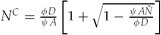 , would in this case be imaginary; this means that for any real-valued number within the Ñ ≤ N ≤