1 Introduction
Sentiment analysis has become an important area of research (Pang and Lee Reference Pang and Lee2008; Bollen, Mao and Zeng Reference Bollen, Mao and Zeng2011; Liu Reference Liu2012) in the last decade, with a high potential of industrial applications. Sentiment analysis is concerned with extracting opinions or emotions from text, especially from user generated web content. Specific tasks include, among others, differentiating opinions from facts, identifying sentiment targets/aspects, detecting positive or negative opinion polarity, determining opinion strength, and monitoring mood and emotion. Currently, two major approaches exist: lexicon and machine learning based. Lexicon-based approaches use high quality, often manually generated sentiment lexicons. Machine-learning-based approaches use automatically generated feature sets from various sources of evidence (e.g., n-grams, parts of speech, emoticons, syntactic parses, negation, and clause types) in order to capture the nuances of sentiment. This means that generally, large sets of features are extracted, out of which only a small subset may be good indicators for the sentiment.
In our work, we focus on the task of predicting user ratings from reviews, based on a machine-learning approach, and more specifically on automatically selecting relevant features for this task. Given the high number of initial features and their low overall quality, feature selection has the potential of having a considerable impact on the performance of a classifier. As a consequence of the large feature set, we will focus on filter methods, i.e., on methods in which the quality of a feature is evaluated by an extrinsic measure, such as information gain (IG), rather than by an evaluation on held-out data (Guyon and Elisseeff Reference Guyon and Elisseeff2003), as in wrapper methods. The specific problems that we will address in this study, the extension of feature selection methods, which generally assume a binary classification, to a multi-class setting, and the challenge that feature selection methods face in a highly skewed setting, are dictated by characteristics of our data set: We use a set of user reviews of online cooking recipes, collected from Epicurious.Footnote 1
On the Epicurious platform, users can leave ratings as well as reviews of recipes. The platform additionally provides an overall rating for a recipe, which is the average of all user ratings. In our setting, the task of the machine learner is to predict the average rating based on the user reviews. That is, we use these ratings as underlying user opinions, and the task is to predict those using textual information from reviews. This is a simulation of situations in which only text but no numeric expression of sentiment is available. This data set is highly skewed: The majority of ratings is positive, and only few ratings are negative. The obvious solutions, using either over-sampling or under-sampling, are not ideal since the minority class constitutes only approximately 1 per cent of the whole data set. Thus, any sampling has an inherent risk of ignoring or downgrading important features. Additionally, we have empirically shown in a previous work (Yu et al. Reference Yu, Zhekova, Liu and Kübler2013) that under-sampling is detrimental to results.
The other important characteristic of the data set is that we have four different ratings, from 1-fork to 4-fork,Footnote 2 which serve as our target classes in a classification setting. As a consequence of the four classes, standard feature selection methods for binary classification are not directly applicable. There are different methods of extending such binary methods to a multi-class setting, and we will investigate those for our problem.
Thus, the underlying questions that we attempt to answer in this study concern the extension of binary feature selection methods to a multi-class setting and the improvement of the classifier for minority classes. The latter will be approached by making features more robust in the sense that we increase their coverage by using part-of-speech (POS) tagging, stemming, and word clustering in addition to or instead of word forms. One underlying challenge with our data set, and potentially with a large range of other data sets in sentiment analysis, lies in the problem that most words by themselves are not good indicators for a single class. Rather, most words tend to occur in several classes, and the few words that occur only in one category tend to be very infrequent and thus do not generalize well. For example, ‘sugar’ or ‘awfully’ may appear in both positively and negatively rated recipes. In contrast, for topic classification, there are words more characteristic of single classes, e.g., ‘parsing’ from an NLP paper is less likely to be used in a high performance computing paper, where ‘GPU’ would be more probable. Using longer n-grams does not change this picture much, but adds data sparsity. Thus, a feature selection method needs to be robust in order to handle such challenging features sets. If there are clear features, it is more likely that most feature selection methods will find them.
The remainder of this article is structured as follows: In Section 2, we present related work. Section 3 describes our research questions in more detail, and Section 4 describes our experimental setup, including data set, preprocessing, classifier, and feature selection details. In Section 5, we present our results concerning the two research questions, and in Section 6, we present a more in-depth analysis of the different feature selection methods. In Section 7, we conclude.
2 Related work
Our work touches on several areas of research: sentiment analysis, feature selection for machine learning, and machine learning for highly skewed data sets. Since all of these fields have a wide variety of publications, we will focus in our review on the most relevant publications. We will start with literature in sentiment analysis, then move on to feature selection in the related field of text classification, and finally discuss feature selection for highly skewed data and in multi-class scenarios.
2.1 Sentiment analysis
Currently, sentiment analysis is approached via supervised learning when annotated data is available. Commonly used classifiers include support vector machine (SVM), Naive Bayes, Maximum Entropy models, and Neural Networks (Mullen and Collier Reference Mullen and Collier2004; Pang and Lee Reference Pang and Lee2004; Ye, Zhang and Law Reference Ye, Zhang and Law2009; Glorot, Bordes and Bengio Reference Glorot, Bordes and Bengio2011). Sequential models, such as Conditional Random Fields, are applied to capture sentiment shifts (Sadamitsu, Sekine and Yamamoto Reference Sadamitsu, Sekine and Yamamoto2008; Nakagawa, Inui and Kurohashi Reference Nakagawa, Inui and Kurohashi2010). In these approaches, feature engineering plays an important role since such approaches often start from surface oriented features, which provide a large feature base but are typically not very informative individually. Typical features fall into several categories: textual cues such as bag-of-words, bag-of-n-grams (e.g., Pang and Lee Reference Pang and Lee2004); syntactic cues such as POS tags, substructures from syntactic parses (e.g. Wilson, Wiebe and Hoffmann Reference Wilson, Wiebe and Hoffmann2005; Nakagawa et al. Reference Nakagawa, Inui and Kurohashi2010); and high-level cues such as word clustering and word embeddings (e.g., Maas et al. Reference Maas, Daly, Pham, Huang, Ng and Potts2011; Socher et al. Reference Socher, Pennington, Huang, Ng and Manning2011). There are also resource-dependent features, such as sentiment scores from a lexicon (e.g., Baccianella, Esuli and Sebastiani Reference Baccianella, Esuli and Sebastiani2010). We follow standard approaches and use word n-grams as our feature base.
2.2 Feature selection
In this section, we describe approaches to feature selection in sentiment analysis and in text classification, which can be regarded as a more general definition of a set of tasks including sentiment analysis.
Text classification is a field that, similar to sentiment analysis, often uses surface features such as a bag of words. Thus, feature selection has received much attention in this field (c.f., e.g., Yang and Pedersen Reference Yang and Pedersen1997; Brank et al. Reference Brank, Grobelnik, Milic-Frayling and Mladenic2002; Zheng, Wu and Srihari Reference Zheng, Wu and Srihari2004; Li et al. Reference Li, Xia, Zong and Huang2009). Feature selection mainly aims to (1) increase computational efficiency by finding a subset of features that perform as well as a much larger set and (2) filter out noise and less relevant features to avoid overfitting. Feature selection is mainly categorized into filter methods and wrapper methods (Guyon and Elisseeff Reference Guyon and Elisseeff2003). Filter methods generally evaluate features by assigning them a ranking score based on the distributional statistics in the data. Wrapper methods identify the optimal subset of features using held-out data. Since the number of subsets is exponential, wrapper methods are extremely inefficient when the feature set is large, even with greedy algorithms. For this reason, we focus on filter methods.
Since filter methods use an external ranking method that is not task-related, one of the concerns is whether such methods prefer frequent or infrequent features. While infrequent features tend to be very characteristic for a class, they may not generalize well to the test data. Highly frequent features, in contrast, generalize well, but may not be very predictive of a class. Filter methods can be based on information theory, statistical tests, or more common principles. Li et al. (Reference Li, Xia, Zong and Huang2009) show that mutual information tends to assign high scores to infrequent words. IG can be interpreted as a weighted average of mutual information, which reduces the bias towards infrequent words. Li et al. (Reference Li, Xia, Zong and Huang2009) and Kummer and Savoy (Reference Kummer and Savoy2012) show that Chi-square and Z-score tend to prefer very frequent features. There are more general methods, for example, odds ratio, the class discrimination measure (CDM) (Chen et al. Reference Chen, Huang, Tian and Qu2009), term strength (Yang and Pedersen Reference Yang and Pedersen1997), and using feature weights from a machine learner. Brank et al. (Reference Brank, Grobelnik, Milic-Frayling and Mladenic2002) finds odds ratio to favor rare words, and they observe a performance improvement when using weights from an SVM classifier to eliminate features of poor quality.
We now turn to sentiment analysis. Certain tasks, such as subjectivity classification, polarity classification, and rating prediction, can be regarded as special cases of text classification. However, the tasks differ in that sentiment analysis usually works with much shorter texts, and words seem to be less specific to a certain class. Thus, not all results from text classification transfer to sentiment analysis.
Most approaches to feature selection in sentiment analysis are filter methods. An exception can be found in the work by Duric and Song (Reference Duric and Song2012), which uses Hidden Markov Model Latent Dirichlet Allocation to separate terms describing entities from terms expressing opinions. Filter methods are dominated by methods based on categorical proportional difference (CPD), which measures a feature’s difference in frequency of occurring in positive versus negative reviews. O’Keefe and Koprinska (Reference O’Keefe and Koprinska2009) compare CPD with two feature selection methods based on manually assigned scores from SentiWordNet. They show that CPD outperforms the other methods in a polarity classification task. Agarwal and Mittal (Reference Agarwal and Mittal2012) propose two variants of CPD: probability proportion difference (PPD) uses the difference of the CPD values for the positive and negative class, and categorical probability proportion difference (CPPD) combines CPD and PPD. Agarwal and Mittal (Reference Agarwal and Mittal2012) show that CPPD performs best in terms of F-measure in a polarity classification task, outperforming CPD, IG, and the baseline using the whole feature set. Kummer and Savoy (Reference Kummer and Savoy2012) focus on a new classification scheme, but they point out that Z-scores tend to assign high scores to frequent terms.
A related task to ours is approached by Severyn and Moschitti (Reference Severyn and Moschitti2015), who use SVMs to learn a sentiment lexicon from twitter data using distant supervision.
2.3 Feature selection for highly skewed data sets
In sentiment analysis, most studies are performed on the Movie Review data set, which has become an established benchmark for sentiment analysis. This set is balanced, consisting of 1,000 positive and 1,000 negative movie reviews. The balance was created via sampling and does not represent the class distribution in the original reviews. For this reason, we focus here on approaches from text classification, where the question of skewing has been approached. Of particular relevance to our work is the work by Forman (Reference Forman2003), who conducted an extensive study of 12 features selection methods on 229 binary text classification data sets, with an average skewing ratio of 1:31. Forman (Reference Forman2003) introduces a new feature selection method, bi-normal separation (BNS), which is the separation between two thresholds in a normal distribution, each corresponding to the probability of a feature occurring in the positive or negative class. Forman (Reference Forman2003) shows that BNS performs within 1 per cent of the best F-measure on 65 per cent of the data sets, while IG is within this margin for 40 per cent of the data sets. In general, the more skewed the class distribution, the more significant the gain that feature selection produces (compared to using the whole feature set). Forman (Reference Forman2003) reports that BNS is more beneficial for highly imbalanced settings. Additionally, while BNS yields higher recall for the minority class, IG yields better precision, and BNS favors more infrequent words, while IG tends to prefer frequent features, therefore leading to a lower dimensionality and thus more efficient models.
Our current work is based on a previous work (Liu, Kübler and Yu Reference Liu, Kübler and Yu2014b), in which we evaluated five feature selection methods (including BNS and IG) on a binary classification task, based on two highly imbalanced sentiment analysis data sets, both from the social media domain. We sampled both data sets to investigate the effect of varying skewing ratios, from 1:1 (balanced), 1:1.57 (slightly skewed), to 1:8 (highly skewed). We found that the benefit of performing feature selection is more significant when the data set is balanced or slightly skewed. We also found that IG is the most stable and best performing method, while the other methods tend to fluctuate. For this reason, we chose IG for our current experiments, which extends our previous work by investigating more robust features and multi-class classification.
2.4 Feature selection in multi-class scenarios
One straightforward extension to our previous work towards multi-class problems is multi-class information gain (M-IG), a metric originating from decision tree learning (Mitchell Reference Mitchell1997). Forman (Reference Forman2004) shows that M-IG tends to promote many features from the easy class and choosing only a few from the difficult classes, making it difficult to fully represent the difficult classes. In Forman’s work, easy and difficult classes are identified according to the F-measure in a multi-class classification task. As a solution, Forman (Reference Forman2004) introduces two variants of round-robin experiments decomposing an n-class classification problem into n 1-versus-all subtasks. The methods vary in how they choose features, either each subtask contributes an equal number of features or the numbers are randomly drawn. Both methods outperform M-IG on nineteen multi-class text classification data sets. Note that these methods are similar to our approaches presented in Section 3.1.
3 Research questions
In this section, we discuss the two major research questions in more detail. The first question focuses on how to extend standard binary feature selection methods to a multi-class scenario. The second question investigates how we can improve performance for the minority classes. Here, the underlying idea is to improve feature representation such that we improve the coverage of the selected features in the minority classes. This means making features more general, for example, by using part-of-speech tags in addition to words.
For all questions, we rely on our previous findings (Liu et al. Reference Liu, Guo, Dakota, Rajagopalan, Li, Kübler and Yu2014a, Reference Liu, Kübler and Yu2014b) and use words as features, either as unigrams, bigrams, or trigrams (but see Section 3.2 for modifications). We concentrate on IG as the metric underlying feature selection since it proved to be the most robust method. We also use a multi-class classifier (for details see Section 4.4). This means that all features chosen in competitions are merged and given in their entirety to the classifier. An alternative architecture would consist of binary classifiers parallel to the competitions in combination with a final voting mechanism. Since the focus of the current work is on feature selection, this approach is beyond the scope of this paper.
3.1 From binary to multi-class feature selection
For this research question, we investigate the following five methods:
-
(1) Binary feature selection (BIN)
-
(2) Automatic feature selection (Lasso)
-
(3) 1-versus-all competition (1-versus-ALL)
-
(4) 1-versus-neighbor competition (1-versus-NBS)
-
(5) Multi-class information gain (M-IG)
For all four methods except Lasso, we use IG. For all settings except for the M-IG, we use the standard definition for two classes. The equation for IG in a binary setting is shown as
 $$\begin{equation}
IG(f) = \sum _{ f \in \lbrace 0,1 \rbrace } \sum _{ C \in \lbrace 0,1 \rbrace } P(f, C)\text{log} \frac{ P(f,C) }{P(f)P(C)}
\end{equation}$$
where f is a feature and C represents one of the two classes. In the case of M-IG, this equation is extended as shown below (Yang and Pedersen Reference Yang and Pedersen1997):
 $$\begin{equation}
IG(f) = \sum _{i=1}^{m}P(c_i)\text{log}P(c_i) + \sum _{ f \in \lbrace 0,1\rbrace } P(f) \sum _{i=1}^{m}P(c_i|f)\text{log}P(c_i|f)
\end{equation}$$
where m ranges over all classes and c i is the ith class. For our task, m = 4.
Every n-gram, from unigrams to trigrams, in the corpus is considered a feature. Probabilities of classes (given features) are calculated as their relative frequency in the training data.
Binary feature selection (BIN):
This is our baseline, which we have used before (Liu et al. Reference Liu, Guo, Dakota, Rajagopalan, Li, Kübler and Yu2014a, Reference Liu, Kübler and Yu2014b). In this case, we perform feature selection based on two classes, the positive class (including reviews for 3-fork and 4-fork recipes) and the negative class (including 1-fork and 2-fork recipes) and then use all selected features for the classification task. This method simplifies feature selection in a multi-class classification scenario to a binary one, assuming that the features selected for either class are still clear enough to help the classifier to choose correctly between all four classes. This method is applicable in our case because we only have four classes, and a 1-fork rating can be considered a more extreme case of a 2-fork rating, etc.
Automatic feature selection (Lasso):
As a more competitive baseline, we perform logistic regression using L1 regularization, which performs implicit feature selection during training of the regression model. The regularization decreases the weights of some features to zero, and those features are ignored. Logistic regression has been shown to successfully perform feature selection in the presence of exponentially many irrelevant features (Ng Reference Ng2004).
1-versus-all competition (1-versus-ALL):
In this setting, we perform four independent, binary feature selection subtasks, in which every class is paired with all other classes. That is, the first round consists of selecting features from 1-fork recipes versus all other recipes. This is a standard solution to multi-class feature selection and similar to multi-class SVMs (Crammer and Singer Reference Crammer and Singer2002), in which an n-class prediction problem is divided into n binary prediction subtasks, with each prediction distinguishing one class from the rest. Afterwards, features selected from each binary subtask are combined into a global feature set.
While the binary feature selection method is more coarse grained (it only distinguishes positive from negative recipes), 1-versus-ALL chooses features for each individual class. However, the downside of this selection method is that we may choose features that are good at separating a class from a far class, for example, 1-fork from 3-fork rather than from the closer 2-fork class. This may be a serious risk for minority classes since the words indicative of positive reviews are more pervasive and thus have a higher chance of being chosen in the selection process for 1-fork versus all other classes. Thus, this method may leave us with many features that occur across classes and are not very discriminative.
1-versus-neighbor competition (1-versus-NBS):
In this setting, we address the concern we have for the 1-versus-ALL setting. Here, we have three selection subtasks, each involving a target class versus its next higher class, i.e., 1-fork versus 2-fork, then 2-fork versus 3-fork, and 3-fork versus 4-fork. Our assumption is that this variant will produce more reliable features for the minority classes than the 1-versus-ALL competition since we use a different search space in each case, thus creating ‘experts’ that can distinguish close neighbors rather than search across the whole spectrum. Note that this method also requires ordered classes.
Multi-class information gain (M-IG):
This is a straightforward extension of IG, i.e., we use equation (2) rather than (1). Here, features are directly ranked with respect to their ability for separating the four classes. Our assumption is that this method will give the best separation into the four classes, but at the same time Forman (Reference Forman2004) has shown that M-IG has a tendency to choose features from the easiest class. Thus, we would expect that many of the features in the global set will be selected from the majority classes.
3.2 Improving performance on the minority classes
For this research question, we investigate how we can improve accuracy on the minority classes given that we have extreme skewing in the data set. Our previous work (Liu et al. Reference Liu, Kübler and Yu2014b) has shown that the choice of feature selection metrics has little effect on the performance on minority classes. Additionally, in many of our initial experiments, we saw that because of the extreme skewing in the data, no examples are classified as 1-fork or 2-fork. Our underlying hypothesis is that with highly skewed data distributions, reviews belonging to a minority class contain many low-frequency features, which means that features selected from the minority classes do not generalize well to new reviews. Consequently, in order to retrieve at least some minority classes, we mostly investigate methods that allow a generalization of the features. We also look at standard sampling methods, such as over-sampling. More specifically, we investigate the following methods:
-
(1) Stemming
-
(2) POS tagging
-
(3) Brown clustering
-
(4) Review sampling
-
(5) Over-sampling
Stemming:
This condition is based on the assumption that feature selection suffers from data sparsity. This can be alleviated by using stemmed forms instead of fully inflected word forms. We assume that the inflections do not carry important sentiment information and that stemming should not harm performance by over-generalizing.
POS tagging:
This is another form of generalizing from a word form. Here, we add POS tags as additional features. We use the Penn Treebank tagset (Santorini Reference Santorini1990), which uses thirty-six POS tags. However, while this approach reduces data sparsity, it is possible that this generalization is too coarse grained since it generalizes both positive and negative adjectives to a standard adjective label (JJ), for example. We use POS n-grams in addition to word n-grams.
Brown clustering:
This is a hierarchical clustering method that clusters words based on their contexts (Brown et al. Reference Brown, Della Pietra, deSouza, Lai and Mercer1992). Brown clustering has been shown to be beneficial for parsing (Koo, Carreras and Collins Reference Koo, Carreras and Collins2008), relation extraction (Sun, Grishman and Sekine Reference Sun, Grishman and Sekine2011), and named entity recognition (Tkachenko and Simanovsky Reference Tkachenko and Simanovsky2012), among other problems. It creates smaller ‘classes’ of closely related words, thus is in granularity between POS tags and full word forms.
Review sampling:
This is an attempt to level out the effect on feature selection methods based on the fact that recipes from the majority classes have a large number of reviews, while recipes from the minority classes have only a few. If we look at recipes with more than ten reviews, we find that only 1.38 per cent of the 1-fork recipes fall into that category, 16 per cent of 2-fork, 49 per cent of 3-fork, and 57 per cent of 4-fork recipes. Consequently, we restrict the maximal number of reviews per recipe to ten randomly sampled reviews, thus mitigating the skewing at the review level. However, the removed reviews may contain valuable information, such as sentiment-bearing expressions not present in the sampled reviews. They may also provide more stable feature frequencies, which are important for rating prediction.
Over-sampling:
A widely adopted method to improve machine learning performance on skewed data sets is to conduct over- or under-sampling. We investigate how much effect over-sampling can have on the minority class in an extremely skewed data set. In this case, we randomly sample from the training data until we have a balanced training set. We do not investigate under-sampling here since in data sets with extreme skewing, under-sampling discards the majority of the whole data set, losing valuable information, as shown by Yu et al. (Reference Yu, Zhekova, Liu and Kübler2013).
4 Experimental setup
4.1 Data set
We have developed a web crawler to collect user reviews for about 20,000 recipes, published on the Epicurious website before and on April 02, 2013.Footnote 3 On the website, each recipe is assigned a rating of 1–4 forks, including the intermediate values of 1.5, 2.5, and 3.5. This is an accumulated rating over all user reviews. We then exclude recipes with ratings of 0, which usually indicate that recipes have not received any ratings. We round down all the half ratings, e.g., 1.5 fork counts as 1-fork, based on the observation that users are generous when rating recipes. We also exclude recipes without reviews or without rated reviews. The latter occur when a user rates a recipe without leaving a comment.
After these clean-up steps, the data set consists of 10,089 recipes, the distribution of ratings in the data set is shown in Table 1. Since 1-fork and 2-fork recipes constitute only 3.4 per cent of the data set, it is obvious that we face a problem with extreme skewing.
The distribution of ratings in the Epicurious data set

The data set is split into training and test sets in a stratified way to maintain the rating distribution. Since the feature selection experiments with all variables we are considering for the current work are extremely time consuming, we have decided to forego cross-validation and use a dedicated split into training and test data with a ratio of 2 : 1, see Table 1. Initial experiments with a three-fold cross-validation setting showed little variation in results.
4.2 Data preprocessing
Before splitting the data into training and test sets, preprocessing is conducted on the whole data set. Text from online reviews is known to be written informally. For example, words and punctuations are not properly spaced: ‘I like this cake, however it needs more butter’. Here, white-space segmentation is not sufficient to separate ‘cake’ and ‘however’. Letters are often repeated and thus create multiple forms of the same word: ‘yummy’, ‘yuuumy’, ‘yuuummmy’. Punctuations can be repeated for emphasis: ‘I love it!!!!!’; again creating multiple word forms. Contractions also increase the vocabulary size by appending the contracted part to the former word: ‘I’ve’, ‘my friend’s’. Additionally, URLs are common in online reviews when authors make recommendations or produce spam. These characteristics in online reviews increase data sparsity. Thus, we use a pipeline that performs the following normalizations:
-
(1) Replace all URLs by a special token ‘URL’.
-
(2) Replace all emoticons by a special token ‘EMO’.
-
(3) Replace all numbers – integers, time intervals, fractions – by a special token ‘KNUMK’.
-
(4) Replace all words and punctuations with repeating letters by their original form.
-
(5) Properly segment sentences, run-on punctuation, and run-on words.
-
(6) Separate all contractions into the first word and the contracted part. For example, ‘don’t’ is separated into ‘do’ and ‘n’t’.
For the experimental settings concerning our second research question (see Section 3.2), we perform stemming using the Porter Stemmer (Porter Reference Porter1980) to normalize words, and POS tagging using the TnT tagger (Brants Reference Brants2000). Since we need to keep the word segmentation consistent between the baseline feature set and the POS tagged set, we had to choose a POS tagger that does not perform segmentation internally, which restricted our choices. Consequently, we use TnT because it is known to perform well on data sets with many unknown words (cf., e.g., Maier et al. Reference Maier, Kübler, Dakota and Whyatt2014)). We use the pre-trained WSJ model.
For the experiments involving Brown clustering, we use the implementation by Liang (Reference Liang2005). The clustering is carried out on the training set after normalization. Then, each individual word in the training and test set is replaced with its cluster number, and the same replacement is carried out for all n-grams. In postprocessing, we grouped all words with a frequency of less than four occurrences in a RARE cluster. Unknown words in the test data were also assigned to this cluster. We have experimented with 1,000 and 1,500 unique word clusters. However, the number of clusters had little effect on classification results.
We do not filter stop words for two reasons: (1) Stop words are domain dependent, and some stop words may be informative for sentiment analysis. For example, users are likely to write more formally in negative reviews, listing specific factors for their negative arguments; thus, punctuations like ‘,’ and ‘.’ are likely to be sentiment-bearing in our data set. (2) Uninformative words that are equally common in all classes should be excluded by feature selection if the method is successful.
4.3 Feature representation
Different feature representation schemes can influence the accuracy in sentiment analysis, but since we focus on feature selection in this paper, we use the commonly adopted bag-of-words approach, extended to word n-grams. Each recipe is represented by all n-grams from its reviews with 1 ⩽ n ⩽ 3. Research in sentiment analysis (Pang, Lee and Vaithyanathan Reference Pang, Lee and Vaithyanathan2002) has shown that using binary feature values performed better than using weighting schemes in a task of classifying positive and negative movie reviews. However, movie reviews are relatively short, so other feature weightings may not necessarily out-perform binary weighting. In contrast, topic classification generally uses term frequency as feature weighting. Given the length of the (combined) reviews from each recipe and the focus of this paper, we use the n-gram frequency as feature weighting. In order to avoid noise and overfitting, we remove all features that occur fewer than four times in the training set.
4.4 Classifiers
Feature selection methods can behave differently in combination with different classification models, because of the underlying differences in parameter estimation and treatment of features. Given the wide success of SVMs (Crammer and Singer Reference Crammer and Singer2002) in text classification and sentiment analysis, we conduct all experiments reported here based on SVMs in the implementation of SVM multi-class V1.01 (Joachims Reference Joachims, Schölkopf, Burges and Smola1999). SVMs are a discriminative classifier that finds hyperplanes to separate different classes by maximizing the margin between the hyperplane and the support vectors. SVMs are capable of successfully using a large number of numeric features and are thus a logical choice given our feature set.
Initial experiments showed that SVM multi-class V1.01 reaches better performance on our skewed data set than the current V2.20 implementation. For this reason, all our experiments are based on V1.01. Because model learning and optimization is not the focus of this study, we use the default linear kernel and other default parameter values. We are aware that the parameterization can affect our results, but finding optimal parameters is a difficult problem, especially given our time intensive experiments, thus we leave this for future work.
For the experiments using logistic regression using L1 regularization (Lasso), we use the logistic regression implementation in Scikit learn.Footnote 4 We use the default parameters where the inverse of regularization strength is 1. Since logistic regression is a binary classifier, the multi-class learner is built by voting on four individual binary classifiers.
4.5 Evaluation
Classification results are evaluated by the micro-averaged F-measure, the macro-averaged F-measure, as well as precision and recall for each class. Note that in classification tasks for which every test case is guaranteed to be assigned one and exactly one class, micro-F is equivalent to accuracy. While micro-F averages over all instances in the test set, macro-F first averages over all instances per class and then averages over all class results. Thus, in calculating macro-F, every class receives equal emphasis while in micro-F, the weight is proportional to the number of examples in the test data. The latter means that in macro-F, the minority classes have the same effect on accuracy as the majority classes, while in micro-F, errors in minority class examples have less influence on accuracy since there are so few such examples. We perform significance tests using McNemar’s test.
4.6 Feature selection
Feature selection is performed on the training data only. We vary the number of features selected from 500 to 5,000 out of a total of 387,000 n-gram features, at a step size of 500. For the 1-versus-ALL and 1-versus-NBS settings, we take an equal number of features (M) from each binary classification subtask, with M ranging between 500 and 5,000. A subtask refers to a 1-versus-rest binary prediction problem, and produces a local feature set. The union of these local feature sets then produces the global feature set. Thus, for 1-versus-ALL, this results in a size of the feature set between M and 4M and between M and 3M for 1-versus-NBS. Note that we report the number of features selected per sub-task instead of the number of features in the global set since some features are selected in more than one subtask, and thus the overall number can be misleading. We will investigate these multiply chosen features in more detail in Section 6.
We generally do not experiment beyond 5,000 features since such experiments are time consuming given the variables that are investigated, and performance generally peaks at about 2,500 or 3,000 features. For completeness sake, we do present results for the full feature set for question 1.
5 Results
5.1 Feature selection methods for multi-class classification
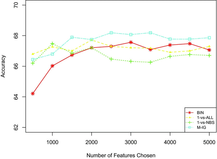
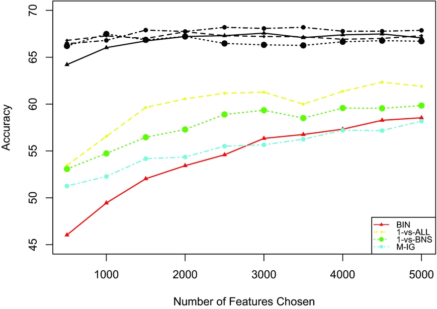
We first evaluate the four methods for multi-class feature selection presented in Section 3.1. For this evaluation, we mainly report micro-F (= accuracy). Figure 1 presents the results (micro-F) of all four feature selection methods when different numbers of features are selected. The results show that the four methods reach their optimal performance with different numbers of selected features: The 1-versus-neighbor method (1-versus-NBS) reaches a performance peak at 1,000 features, 1-versus-ALL reaches the peak at 2,000 features, and M-IG and the binary method (BIN) peak at 2,500 and 3,000 features, respectively. This comparison also shows that the binary selection method is surprisingly successful once a larger set of features is available. 1-versus-ALL and 1-versus-NBS are both initially competitive, but less so with a larger feature set. All these observations show that using an inherently multi-class feature selection provides a better feature set than using an approximation via several binary choices.
Comparing methods for multi-class feature selection (micro-F).

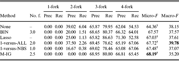
Table 2 shows the results for the four feature selection methods in more detail, with BIN and Lasso as baseline. For Lasso, the number of selected features ranges between 46 and 1,059, with the number of features correlating with the size of the class. The None setting uses the entire set of n-gram features, around 387,000. The results show that using all features (None) results in the lowest micro-F, which shows that the large set of features potentially contains irrelevant ones that affect the performance of the SVM. Lasso shows a similar performance to BIN, with a slightly lower micro-F and a slightly higher macro-F, thus showing that L1 regularization does not work well in our setting. For this reason, we will not continue this option further.
Results comparing feature selection methods for multi-class classification

The highest micro-F score is shown in bold. (The number of features is reported as per thousand.) †Significant on the 0.1 level as compared to BIN.
For the feature selection models, we focus on the optimal number of features per method, and we include precision and recall for the individual rating classes as well as macro-F. For the majority classes, we see that the trends for BIN and M-IG are different from those for 1-versus-ALL and 1-versus-NBS: BIN and M-IG have lower precision and higher recall for 3-fork; with the opposite trend for 4-fork. This shows that BIN and M-IG have a tendency to choose the 3-fork class, while the other two methods prefer 4-fork. The results for macro-F are approximately 30 per cent points lower than the micro-F results, thus showing that the low performance on classes 1 and 2 is extremely detrimental. We also see that given this evaluation, 1-versus-ALL performs better than all other methods, increasing results from 37.57 for BIN to 39.78 for 1-versus-ALL.
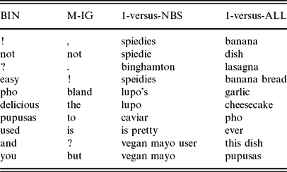
Table 3 shows the ten features that reach the highest IG per feature selection method. For 1-versus-ALL and 1-versus-NBS, the highest value for a feature reflects the highest score out of all subtasks. It is obvious that both BIN and M-IG chose a high number of stop words, while the other two methods tend to select less common words, such as ‘pho’. We will investigate the features selected by M-IG more closely in Section 6.1.
Top ten features chosen by different feature selection methods

The analysis in Table 2 also shows that none of the four feature selection methods allows the classifier to predict any 1-fork ratings. Additionally, all feature selection methods except M-IG allow finding some 2-fork examples, albeit with extremely low recall. Using multi-class information gain, the method with the highest accuracy over all classes, in contrast, results in not finding any 2-fork examples. In a setting where we may be interested in reliably identifying unsuccessful recipes, which should not be suggested to other users, this situation is far from being satisfying. For this reason, in the following section, we will investigate improving the situation for the two minority classes, 1-fork and 2-fork.
5.2 Improving performance on minority classes
In this section, we investigate whether methods for generalizing our lexical features will lead to improvements for the minority classes: We investigate stemmed words, POS tags, and word clusters based on Brown clustering (Liang Reference Liang2005) and compare them to the baseline where the features consist of word n-grams. These methods are based on the assumption that our feature selection methods are not able to find features that represent the 1-fork and 2-fork classes well. Since we have fewer recipes in these classes, we consequently have fewer features extracted from them, and it is less likely that these features will occur in test reviews. Thus, if we can make those features more general, and consequently more robust, we may have a better chance of identifying examples of the minority classes. Additionally, we investigate more traditional sampling methods, where we either sample the number of reviews per recipeFootnote 5 or we over-sample the minority recipes. Note that the goal here is to improve performance on the minority classes, even if this means a decrease in overall accuracy.
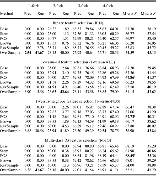
Table 4 shows the results of all methods. We focus here on a set of 2,500 features across all experiments since this is a good compromise given the results in Section 5.1. These results show that using POS tags in combination with either 1-versus-ALL, 1-versus-NBS, and M-IG actually result in a slight increase of accuracy over the least robust method using word forms as features (shown as Base in the table)Footnote 6 .
Results for improving performance on minority classes (using 2,500 features)

†Significant on the 0.1 level as compared to BIN. ‡Significant on the 0.05 level as compared, bold = highest value for this metric, to BIN and as compared to the next lower POS result.
When we look at the performance of the generalization and sampling methods on the 1-fork class, we see that only over-sampling results in finding 1-fork examples across all feature selection methods. Using over-sampling, we gain considerably in recall (ranging from 5.56 per cent for 1-versus-ALL to 41.67 per cent for BIN and M-IG), but precision is extremely low (ranging from 6.36 per cent for M-IG to 7.54 per cent for BIN). Looking at the 2-fork class, the picture looks more promising. Recall remains low for all generalizations but reaches values between 40.00 per cent for BIN and M-IG and 42.64 per cent for 1-versus-ALL when we use over-sampling. When we look at precision for the 2-fork class, the highest values are reached by using review sampling, ranging from 35.71 per cent for BIN to 61.91 per cent for 1-versus-ALL. Any success for the minority classes directly translates into a gain in macro-F: Both sampling methods consistently outperform the baseline.
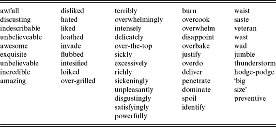
In general, stemming shows some improvement for the 2-fork class while keeping accuracy stable. Using POS tags does not show any obvious improvement for the minority classes but results in small gains in accuracy. In contrast, Brown clustering, either with 1,000 clusters or with 1,500 clusters, shows little or no improvement over the baseline. We assume that this is due to the low quality of Brown clusters, which are obtained from a relatively small training set. Table 5 presents examples of clusters. These examples show that on the one hand, these clusters group misspelled words with the correct variant, such as ‘loiked’ and ‘liked’, thus reducing data sparsity. On the other hand, they group words with positive sentiment along with negative words into the same cluster, for example ‘disliked’ and ‘liked’. Such clusters may not be useful for rating prediction.
Examples of word clusters created by Brown clustering

Review sampling shows the highest improvement on the 2-fork class but also results in a decrease of accuracy in the range of 4 per cent points. On the one hand, the number of reviews per recipe for each class is more balanced, resulting in a less skewed corpus. On the other hand, by restricting to ten reviews, we lose a great amount of information for the majority class, which is important for the separation between 3- and 4-fork classes. Thus, we see a drop in performance for these two classes. Over-sampling is the most successful method for minority classes, especially with regard to recall, but the drop in accuracy is even more pronounced than for review sampling, reaching almost 13 per cent points for the M-IG feature selection.
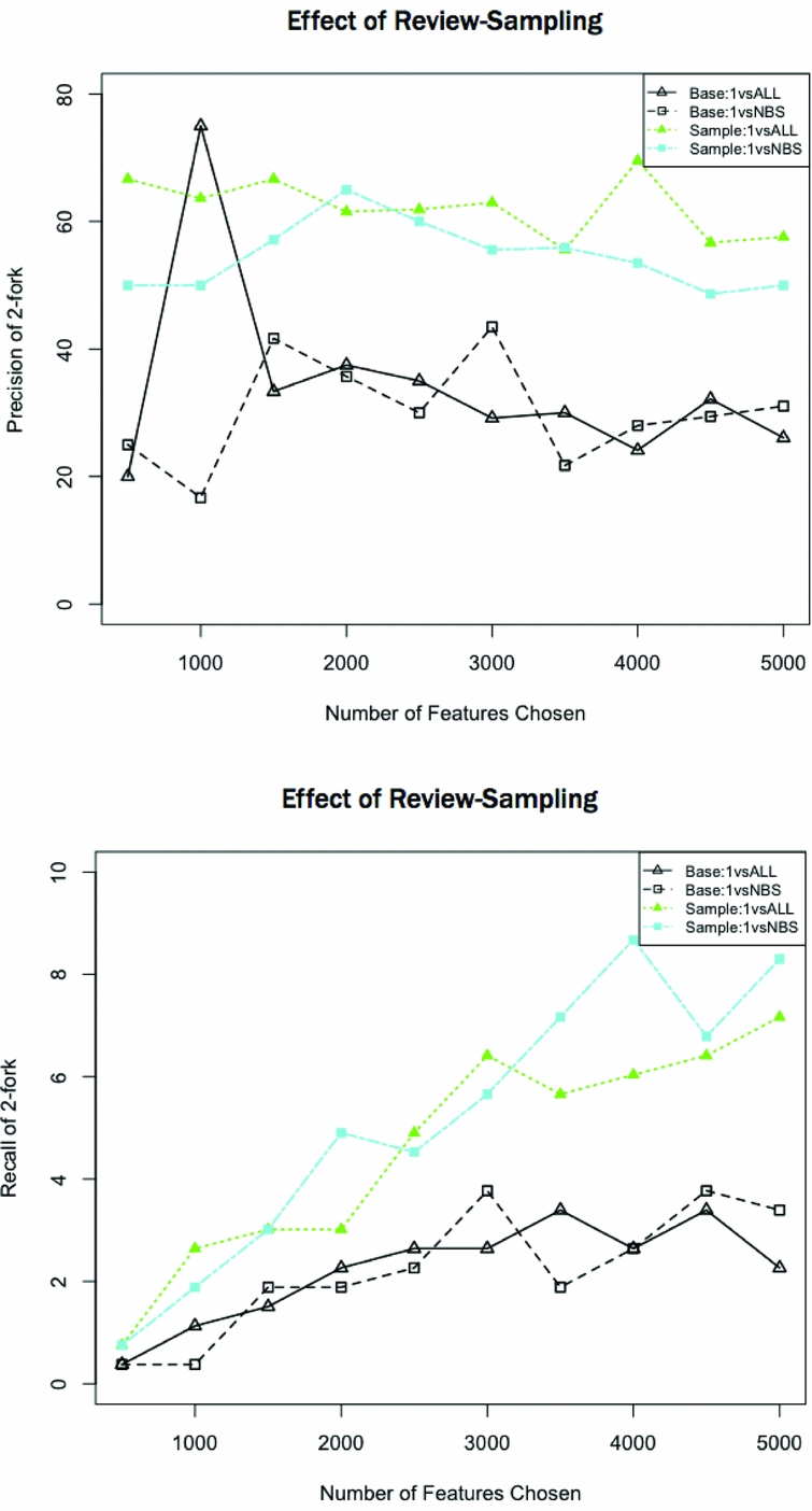
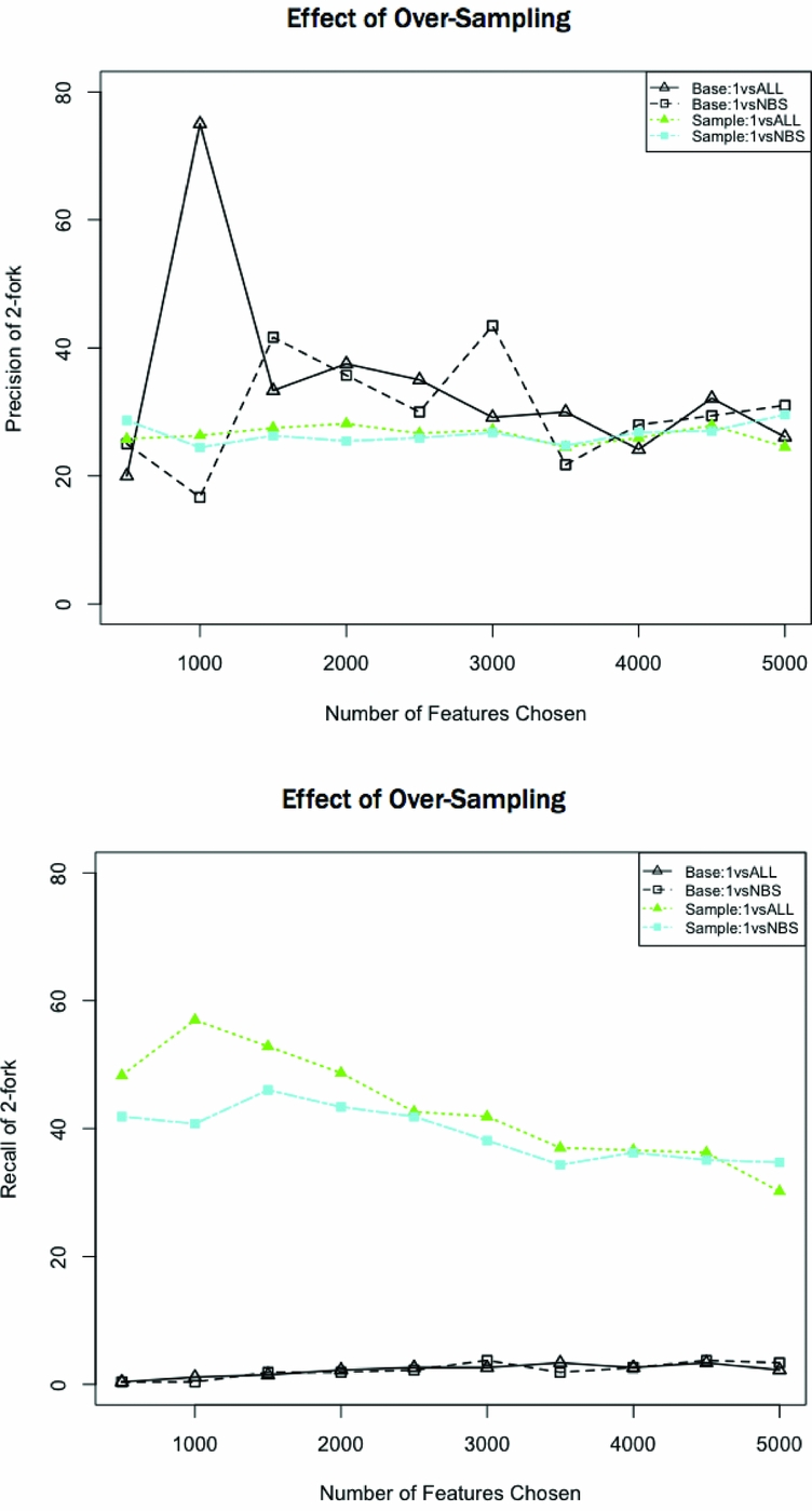
We further need to establish whether the observed positive behavior of the two sampling methods is stable across different numbers of selected features. Figure 2 shows a comparison of the precision and recall values between the baseline and the sampling methods for 1-versus-ALL (solid lines) and 1-versus-NBS (dotted lines) for the 2-fork class for review sampling, and Figure 3 for over-sampling. The graphs show that precision is stable for both sampling methods; recall increases steadily for review sampling and decreases for over-sampling. However, for both methods, recall is clearly superior compared to the baseline.
Effect of using review sampling on the precision and recall of the 2-fork class.

Effect of using over-sampling on the precision and recall of the 2-fork class.

We also had a closer look at the accuracies for over-sampling given increasing numbers of selected features. These results are shown in Figure 4. This graph shows that while the baseline methods (the four highest curves) remain stable across feature sizes, over-sampling in combination with all feature selection methods increases steadily with an increase in the number of features. However, even the best method using over-sampling, 1-versus-ALL, remains below the accuracy of the baselines without over-sampling. This may mean that over-sampling requires more features than the unsampled baselines. But since using a high number of features is costly when using SVMs, we refrain from increasing the feature sets further, especially given the results from Figure 2, which show that recall for the 2-fork class decreases while precision remains stable. Thus, adding more features will only increase a preference for the majority classes.
Loss in accuracy using over-sampling.

To conclude, the two most successful feature selection methods are 1-versus-ALL and 1-versus-NBS, in combination with review sampling for high precision and with over-sampling for high recall. The method with the highest performance in terms of accuracy, M-IG, in contrast, cannot profit very much from the methods presented here. These results lead to further questions, namely whether we can improve the performance of the M-IG feature selection, whether it is possible to combine the strengths of M-IG and 1-versus-NBS, and how well the selected features are distributed across different classes. We will investigate these questions in the following section.
6 Further analysis
6.1 M-IG analysis
Our results in Section 5.1 show that M-IG is the highest performing feature selection method where accuracy is concerned. However, we have also seen that M-IG reaches its high performance by exclusively grouping recipes into the majority classes, 3-fork and 4-fork. This leads us to the assumption that this method is not able to represent the minority classes suitably and that performance on the minority classes can be improved if we increase the contribution of the features selected from those classes. In order to investigate this assumption, we implement a variant of under-sampling, in which we sample the features from recipes of different classes rather than the individual recipes or reviews. This gives us control over the ratios of features from different classes. We can, for example, reach a feature ratio of 1 : 1 : 1 : 1, which means that all classes provide the same number of features, with the smallest class (1-fork) controlling the overall number. However, note that the ratio mentioned above is an idealization because a feature may be selected for more than one task and is thus counted towards each class with which it occurs. Originally, if we use all features from the different classes, we have the ratio 1 : 15 : 228 : 222.
We experiment with sizes between 400 and 800 features per class. However, since the smallest class controls the amount of features selected, the range of feature set sizes per class is smaller than in the experiments reported in Section 5. We investigate using the same number of features for all classes (1 : 1 : 1 : 1), allowing twice as many features for all classes except 1-fork (1 : 2 : 2 : 2), three times as many (1 : 3 : 3 : 3), and four times as many (1 : 4 : 4 : 4). Consequently, this method emphasizes the contribution of the minority classes to the feature set, but it has the possible drawback that we ignore many (highly discriminative) features from the majority classes.
The results of these experiments are shown in Table 6. Since low feature set sizes consistently produced low results, we refrain from reporting them here and focus instead on 600, 700, and 800 features per class. For the same reason, we do not show the results for ratio 1 : 1 : 1 : 1.
The effect of down-sampling feature sets for M-IG

bold = highest+second highest value for this measure
The results for under-sampling show that the lower ratios result in a lower accuracy than the baseline, which reached an accuracy of 68.19 per cent in Table 2. However, at a size of 700 features, we observe a slight increase of accuracy over the baseline for both higher ratios, in the case of using four times as many features coupled with an improved performance for the 2-fork class. This setting reaches a precision of 28.57 per cent and a recall of 0.75 per cent. For the sizes of 600 and 800 features and higher ratios, in contrast, we see a decrease in accuracy, but an increase in precision for the 2-fork class to 50.00 per cent for 1 : 3 : 3 : 3 and to 33.33 per cent and 11.11 per cent for 1 : 4 : 4 : 4.
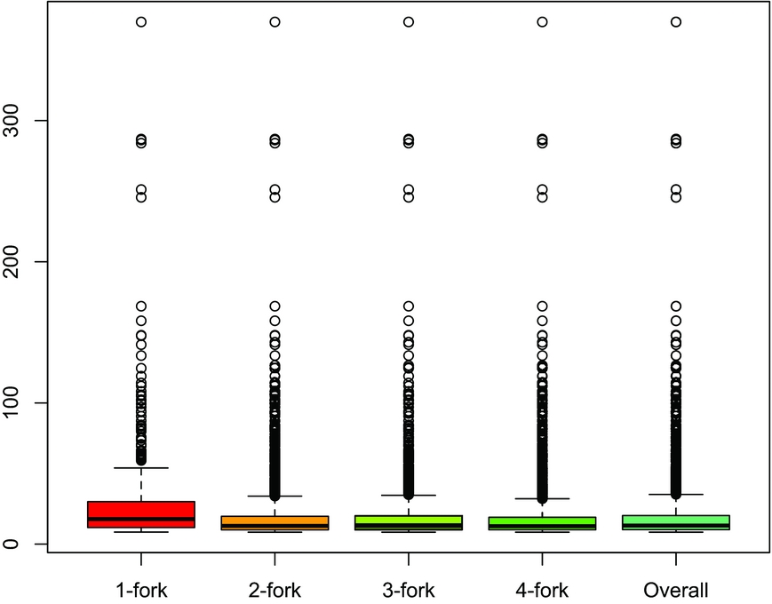
The results from the above experiments show that under-sampling the features from each class does not improve accuracy (with the exception of a minimal improvement using 700 features). To have a closer look, we plotted the IG of the highest ranked features per class in Figure 5. For readability the scale on the y-axis is multiplied by 107. In the box plot, the thick black lines in each box are the medians, and quantiles are delimited, by the bars, the boxes, and the median. Any values beyond the two bars are outliers.
Information gain values for features chosen by M-IG, outliers reflect the common words.

Figure 5 gives an indication that the top features chosen by M-IG are identical for all four classes. Table 3 in Section 5 additionally shows that the ten highest ranked features for M-IG are all stop words with very high frequencies. In the calculation of M-IG for each term, the conditional probabilities are weighted by p(f). It seems that the latter term outweighs any discrimination produced by the other terms. Thus, one drawback of M-IG is that it is biased toward extremely frequent words, which tend to be stop words. As described in Section 4, we did not remove these stop-words in preprocessing because we believe a good feature selection method should be able to filter out non-discriminative features including stop words. However, we did carry out an additional experiment, in which we removed punctuation and stop words using the nltk stop word list (Bird, Klein and Loper Reference Bird, Klein and Loper2009). These results were consistently about 2 per cent points lower, thus showing that the stop words were not the (only) cause for the low results. We still see many frequent words, which are not stop words.
We also experiment with a setting in which we relax the constraint that features need to occur at least four times in the minority classes in order to encourage more contribution from these classes. This method, however, leads to consistently lower results, both in terms of accuracy and in terms of performance on minority classes. We assume that the additional features do not generalize well and are thus not useful in testing. Additionally, we experiment with redefining the sample size of features for calculating the probabilities P(f) and P(c|f) in equation (2): Instead of using the frequency of each term in a given class, we normalize it by the number of documents in that class. For instance, ‘Love it. Love it. Love it’ is a more strongly positive sentiment than just ‘Love it’. The standard approach rates both cases similarly, while the normalization achieves a middle ground between the two approaches. However, this setting resulted in a slight improvement for some settings of the lower ratios, but these results did not reach the results of the higher ratios in the downsampled setting.
6.2 Combination of methods
In this section, we have a closer look at combining feature selection methods in order to combine their strengths. The results presented in Section 5.1 show that M-IG results in high accuracy, especially for the majority classes, but 1-versus-NBS has the best performance on the minority classes. This raises the question whether we can combine the strengths of both approaches. Such a combination can be performed in two ways: (1) We can take the intersection of the features sets, which means that we keep features that are chosen by both M-IG and 1-versus-NBS. That is, we focus on features that are rated highly by both methods. (2) Or we take the union, i.e., we keep features chosen by either M-IG or 1-versus-NBS. In this setting, we obtain a larger set of features since they are chosen by at least one method.
The experiments are conducted with the number of features varying from 500 to 5,000, the results are reported for 2,500 features to ensure comparability with previous analyses. The trends for the other feature set sizes show very similar regularities.
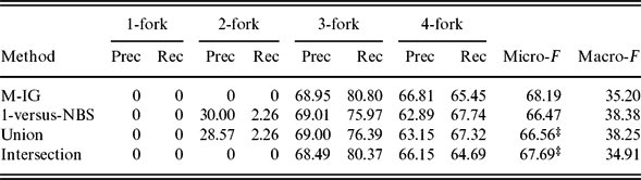
The results in Table 7 show that neither the intersection nor the union of features from the two methods yields the expected increase in performance. Both methods reach a higher accuracy than the 1-versus-NBS methods, but they cannot reach the accuracy of M-IG. However, it is interesting to see that the union reaches similar results for the individual classes to 1-versus-NBS, while the intersection is closer to M-IG.
Combining multi-class IG and 1-versus-NBS for feature selection

‡Significant on the 0.05 level as compared to M-IG.
Figure 6 shows the coverage of features in terms of the percentage of features in the global feature set occurring in each class. For example, for 1-versus-NBS, less than 20 per cent of the global feature set constitute features from 1-fork recipes. Again, a feature can be shared by multiple classes and is then counted toward every class in which it appears. This means that the percentages of one setting do not add up to one hundred. The figure corroborates that M-IG and the intersection have very similar feature distributions and that 1-versus-NBS and the union are equally similar. If we take the results from Table 7 and Figure 6 into account, we can conclude that the features selected by M-IG almost constitute a subset of the features selected by 1-versus-NBS. This also means that the additional features in 1-versus-NBS improve performance for the minority classes, but that simply adding them to the mix is insufficient to improve overall results; they need to be given proper weight.
Feature coverage for different settings combining M-IG and 1-versus-NBS (as ratios of the full sets).

6.3 The role of multiply occurring features
The motivation for using feature selection was based on our assumption that the feature selection process would identify highly discriminative features for the individual classes. However, when we had a closer look at the features selected in the experiments in Section 5.1, we noticed that individual features often occur in more than one binary feature selection subtask. A subtask is one binary feature selection in the 1-versus-ALL setting that selects features that can tell one class apart from all other classes (e.g., 1-fork versus all other classes). This observation led us to investigate how useful or harmful these features selected by multiple subtasks are for the classification task. There are two possibilities: (1) They are not specific for distinguishing a particular class and thus harmful in the multi-class prediction task. Therefore, by removing such features, we expect an increased accuracy. (2) The features are discriminative, potentially in combination with other features, of multiple classes at the same time and are thus useful in the multi-class prediction task. Thus, by focusing on these multiply chosen features, we should reach an increased accuracy. We will look into the following settings:
-
(1) Remove>1
In this setting, features that are chosen by more than one binary subtask are removed. Thus, we only keep features unique to one subtask.
-
(2) Remove>2
In this setting, we allow more overlap and only remove features that are chosen by more than two subtasks.
-
(3) Keep>1
This setting is the counterpart of experiment ‘Remove>1’: We only keep features chosen by more than one subtask.
-
(4) Keep>2
This setting is the counterpart of experiment ‘Remove>2’: We keep the features chosen by more than two subtasks.
In this analysis, we concentrate on the 1-versus-ALL setting, which has been shown to be the most robust next to the M-IG setting, which has been analyzed in the previous section. We report results for 2,500 features to ensure comparability to the experiments in Section 5.1. We have conducted experiments with varying feature numbers from 500 to 5,000 and observed similar trends.
We show the effects of manipulating the multiply chosen features on accuracy in Table 8. The baseline repeats the results for 1-versus-ALL from Section 5.1. Surprisingly, we see that removing the features chosen by multiple subtasks has a detrimental effect on accuracy: Remove>2 results in a decrease in accuracy of around 5–6 per cent points, while Remove>1 results in an even more extreme loss of around 15–16 per cent points. These findings support the hypothesis that such multiply chosen features, especially in their entirety, are useful discriminators in a multi-class prediction task. This is corroborated by our findings for the cases where we only keep multiply occurring features. In the case where we keep features chosen by more than one subtask, our results increase by almost 1 per cent point. This is a clear indication that these features, even though they are not very discriminative by themselves do support multi-class prediction. That is, even though some features have high IG values, they may be good predictors of the ALL class rather than the class that is separated out. This would explain why they are chosen by more than one subtask. Additionally, one drawback of filter-based feature selection methods is that they do not examine combinations of features, but only look at them individually.
Analyzing the role of multiply occurring features

†Significant on the 0.1 level as compared to 1-versus-ALL; ‡Significant on the 0.05 level as compared to 1-versus-ALL.
We also had a closer look at the performance of the classifier on different classes. These results are also shown in Table 8. They show inconclusive trends: While removing the multiply occurring features has a detrimental effect on the majority classes, keeping only features occurring in more than one class has a positive effect on them. With regard to the minority classes, both removing all features in more than one subtask and keeping only features that occur in more than one subtask has a positive effect on precision for 2-forks, while removing features that occur more than once has a positive effect on recall for 2-forks. However, since the number of examples affected is rather small, we assume that this is not a stable effect: 1-versus-ALL correctly predicts seven out of twenty 2-fork instances, Keep>1 correctly predicts six out of fourteen instances. Thus, we can conclude that removing multiply occurring features has a minimally positive effect on the minority classes. This can be attributed to the fact that the deleted features generally originate from the majority classes. Thus, we obtain a focus on pure minority features.
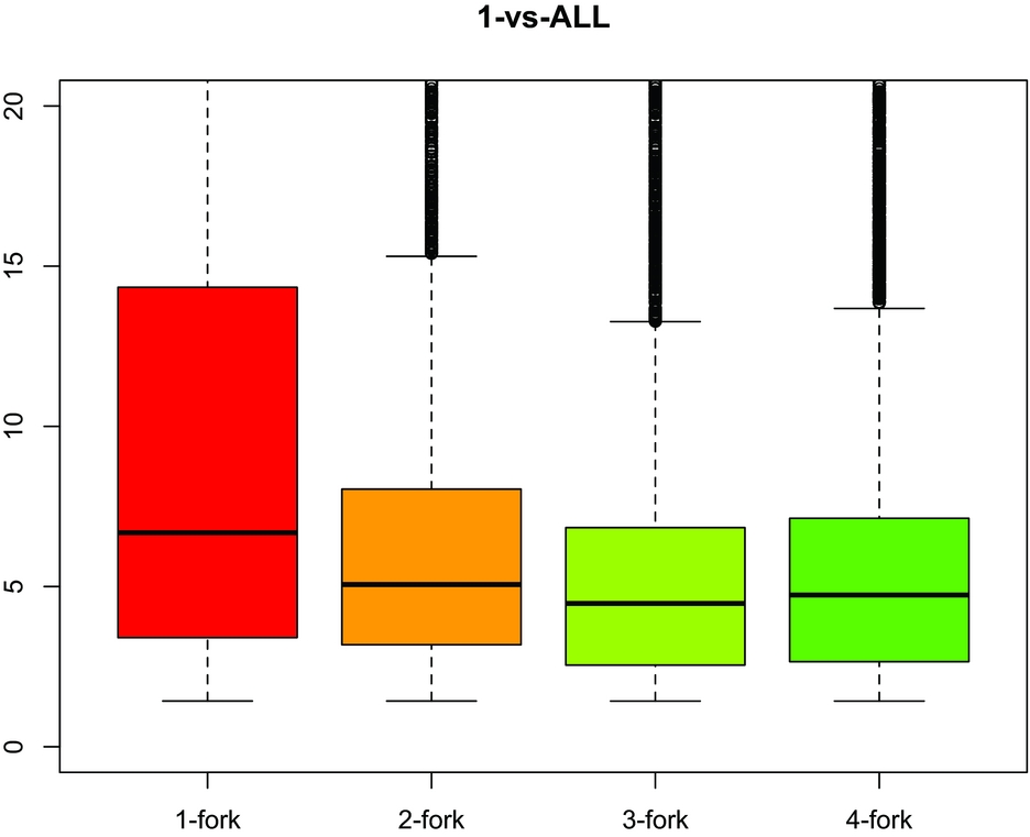
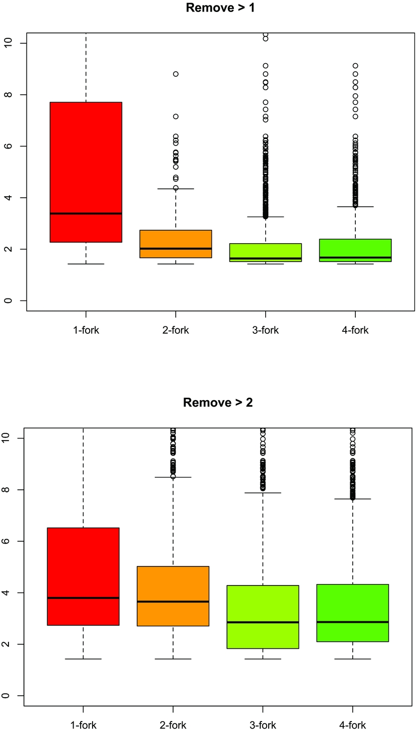
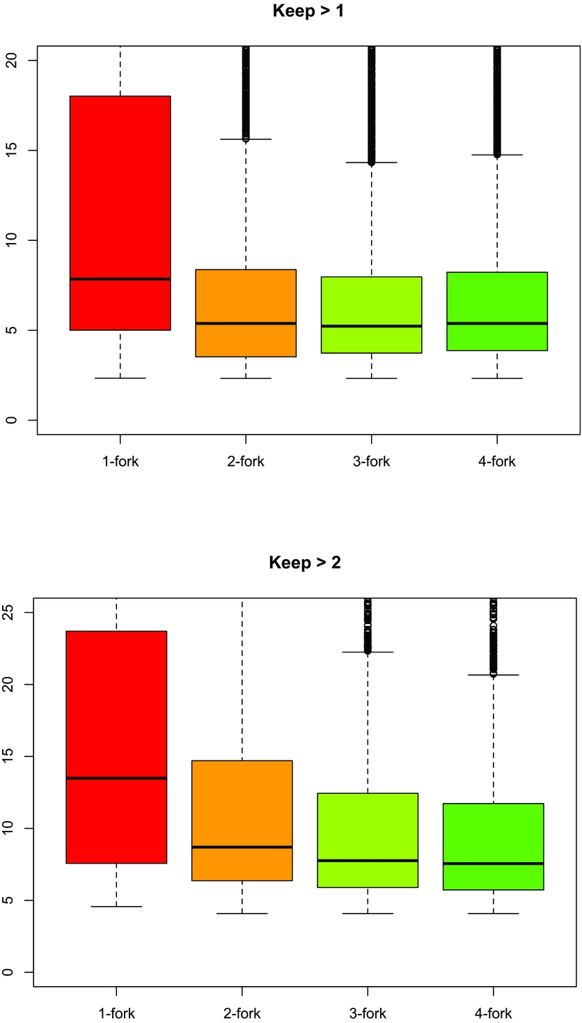
To further understand this phenomenon, we examine the feature distribution across classes in relation to their IG values. Figures 7–9 illustrate the IG values for features per class obtained in each setting. This analysis focuses on the quality of features per class. Again, the scale on the y-axis is multiplied by 107. The analysis in Figures 7–9 shows that the feature coverage is relatively similar for each setting. However, there are major differences in feature quality for the individual settings. The base setting produces feature values around IG values of 5(× 10−7), with Remove>2 having slightly lower IG values between 3 and 4. The Remove>1 setting has the lowest IG values, below 2 for most classes. In contrast, for the multiply occurring features, Keep>1 reaches IG values of above 5, and Keep>2 at around 10; the latter are the highest values across all settings. Note that these findings correlate with the accuracies shown in Table 8.
Feature quality in the 1-versus-ALL setting for multiply occurring features.

Feature quality in settings where multiply occurring features are removed.

Feature quality in settings where multiply occurring features are kept.

These findings suggest several conclusions: (1) In a 1-versus-ALL setting for feature selection, the more subtasks a feature is chosen in, the higher its IG value is. This supports our finding that multiply selected features are indeed beneficial for a multi-class classification. (2) Keep>2 yields a set of high quality features – using a much smaller feature set as shown in Table 9 – and maintains competitive results. Thus this setting has the best time performance among all others. (3) The quality of the features used in each setting is directly indicative of the multi-class classifier performance. Thus, a look at this quality can indicate whether a set of features will perform well in classification.
The absolute size of features per class

In Figures 7–9, we also notice that the 1-fork minority class has the lowest performance but is represented by the highest quality features compared with other classes. In contrast, the majority classes 3- and 4-fork are represented by features of low quality. To understand this situation better, we look at the coverage of features across classes. We define coverage as the percentage of the global feature set that occurs with a class. The feature coverage is shown in Figure 10. Note that one feature can occur in more than one class and is counted toward all classes in which it occurs. Thus, the percentages in Figure 10 do not necessarily add up to one hundred.
Feature coverage for different ways of handling multiply occurring features.

This analysis shows that even though the features that represent the 1-fork class have high IG values, there are only very few of them. Also, the percentage of 1-fork features remains equally low across all settings, whereas the percentages of features for the other classes increase. Keep>2, which reaches the highest accuracy, also has the highest percentage of majority class features. We also notice that in the Keep>2 setting, 4-fork produces more features than 3-fork, which translates into higher precision for 4-fork in this setting (see Table 8).
We also looked at the absolute number of features for the different settings, shown in Table 9. These numbers corroborate that the number of features for 1-fork is low across all settings, in comparison to the features for other classes. Note that the number of 2-fork features is the highest for the baseline, closely followed by Keep>1, which reaches the highest precision and recall values for this class across all settings (see Table 8).
From these findings, we can draw the conclusion that there are not enough features from the minority classes in any setting to reach a good coverage. Thus, in cases of extreme skewing with a small number of training instances, even high quality features cannot mitigate the low coverage. In addition, these features from the minority classes do not generalize well on test data. For example, of the 32 out of 2,500 features from 1-versus-ALL that are exclusive for 1-fork recipes, 20 do not occur at all in the test data, 2 features occur between 3 and 5 times, and 8 features occur once or twice. Given that there are 3,368 test instances in total, the contribution of these features toward 1-fork ratings is minimal.
To conclude this section, we have shown that features chosen by multiple binary feature selection subtasks are good discriminators for multi-class prediction. We have also shown that the quality of features correlates with the classification performance. However, feature quality alone is not sufficient to boost the performance for minority classes, because of a lack of feature coverage for those classes. While Keep>2 is the setting with the highest feature quality, we lack high quality features that are exclusive for each class. This implies that this type of sentiment analysis is a difficult task, likely due to the fact that reviewers use similar expressions in comments reflecting various ratings. In contrast, spam detection is a well-known classification task, which is also subject to extreme skewing, but which can be solved effectively. This task seems to have more features that are exclusive in spam and non-spam (such as ‘21 million dollars’, ‘prize!!!’, or ‘viagra’), which cover up the effect of extreme skewing. However, a confirmation of this assumption is outside the scope of the current work.
7 Conclusion
In this study, we have investigated a variety of methods for multi-class feature selection for sentiment analysis when the data set is highly skewed in terms of the class distribution. We have also investigated the effect of feature selection on the performance of minority classes. We have used a data set of cooking recipe reviews, which provides us with novel challenges: On the one hand, the reviews differ from other text classification data sets in that they do not have surface-level features that are exclusive for a single class. Instead, many surface-level features occur across different classes, which provides a challenge for feature selection methods. On the other hand, we decided to use the extremely skewed data set rather than sampling from the data set to reach an equal class distribution. Thus, we focus on a more realistic view of the problem of sentiment analysis than the previous work.
Our results show that M-IG is the best feature selection method in terms of overall accuracy. At first glance, these results seem to contradict the findings by Forman (Reference Forman2004), who found for document classification that a Round-Robin version of 1-versus-ALL performed better than M-IG. However, they show the same trend: Forman (Reference Forman2004) found that M-IG is good at predicting easy classes, which correspond to the majority classes in our data set. Since our data set is extremely skewed, the benefit of M-IG for majority classes outweighs the benefit of 1-versus-ALL and 1-versus-NBS for minority classes. Consequently, we observe a higher overall accuracy from M-IG.
In analyzing the features, we have found that M-IG tends to select the most common features, including stop words. This is a drawback since a good feature selection method should be able to filter out stop words by itself. It also explains why this method cannot profit from selecting features from minority classes since this restriction would again mainly choose highly frequent words. In contrast, 1-versus-ALL and 1-versus-NBS tend to select more rare features, with a higher percentage of words that represent the minority classes.
A closer look at the 1-versus-ALL method shows that many features with high IG values tend to occur in more than one class, thus corroborating our suspicion that in our task, there are no highly discriminative features for individual classes. Many words or phrases are shared among reviews of all ratings. Consequently, we need a larger set of words, which reach a high accuracy in classification in combination with other words. These findings also indicate that we can restrict the size of the feature set, thus reducing training and testing time while maintaining performance, by using features that are selected in more than two binary prediction subtasks.
Finally, to address the issue of extreme skewing, we have seen small improvements using 1-versus-NBS and 1-versus-ALL along with POS tagging or stemming to make our features more general. However, no setting produces satisfactory results on minority classes. We show that features from the minority classes are of high quality, with regard to IG, but they still reach the lowest coverage in the global feature set. Thus, we need to conclude that feature selection is not able to mitigate the effect of extreme skewing since we cannot increase the coverage of the features even by making the features more general. In such cases, collecting more data (if possible) seems to be the only way to reach better performance for the minority class. However, this also shows that using an evenly sampled data set (with regard to class distribution) means ignoring an important and extremely challenging problem and that results gained under such conditions may not generalize to the more realistic, skewed scenario.