



1. Introduction
When one phase of fluid is injected into an ambient gas environment through a circular tube, a cylindrical jet with axial velocity can be formed. Adding circumferential rotation to the jet, a swirling jet with azimuthal velocity can be further produced. The swirling jet is widely encountered in natural phenomena such as tornadoes and hurricanes (Karami et al. Reference Karami, Hangan, Carassale and Peerhossaini2019; Zhang et al. Reference Zhang, Wang, Liu, Xu, Khoo and Du2023). It also plays an important role in engineering applications such as the reduction of noise (Lee et al. Reference Lee, Lee, Woo, Han and Yoon2024; Li et al. Reference Li, Shen, Cheng, Gao, Liu and Yan2024), the improvements of combustion efficiency (Borsuk et al. Reference Borsuk, Williams, Meadows and Agrawal2015; Balakrishnan & Srinivasan Reference Balakrishnan and Srinivasan2016) and atomization efficiency (Ghaffar et al. Reference Ghaffar, Kasolang, Hamid and Eshak2023; Shim et al. Reference Shim, Kim, Kim, Kim, Ryu and Lee2023). Therefore, it is crucial to investigate the instability characteristics of the swirling jet.
Comparing with the non-swirling jet which has been widely investigated for more than 100 years (Lin Reference Lin2003; Eggers & Villermaux Reference Eggers and Villermaux2008; Montanero & Ganán-Calvo Reference Montanero and Ganán-Calvo2020), the instability of the swirling jet is much more complicated owing to the addition of an azimuthal velocity component. For the swirling jet of a homogeneous medium without the formation of an interface, numerous kinds of velocity profiles have been utilized to model the azimuthal flow. For example, the well-known Batchelor vortex was used in some early studies considering the temporal and spatiotemporal instabilities of the jet (Khorrami Reference Khorrami1991; Olendraru et al. Reference Olendraru, Sellier, Rossi and Huerre1999; Yin et al. Reference Yin, Sun, Wei and Wu2000). The Taylor vortex and the Lamb–Ossen vortex have also been utilized to approximate the basic azimuthal velocity profile of the swirling jet (Hu, Sun & Yin Reference Hu, Sun and Yin2001; Sun et al. Reference Sun, Hu, Gao and Yin2002). Since the Rankine vortex which consists of a core in solid-body rotation (i.e. the flow rotates with a constant angular velocity) surrounded by a potential flow with constant circulation can approximate the final state of swirling flow, it has been most commonly used for the jet azimuthal velocity profiles. Loiseleux, Chomaz & Huerre (Reference Loiseleux, Chomaz and Huerre1998) conducted a spatiotemporal instability analysis of an inviscid swirling jet based on the azimuthal Rankine vortex and the axial discontinuous velocity profile. They derived an analytical dispersion relationship of perturbation development and studied the transition between absolute instability (AI) and convective instability (CI). Gallaire & Chomaz (Reference Gallaire and Chomaz2003a) considered a similar model but assumed that there was a sudden jump of circulation outside the vortex core. They identified four physical mechanisms of jet instability, i.e. the Coriolis effect and the centrifugal effect caused by vortex core rotation, and the axial and the azimuthal Kelvin–Helmholtz instabilities (KHIs) caused by velocity difference. Gallaire & Chomaz (Reference Gallaire and Chomaz2003b) considered a model which could describe the intensity of shear stress in the azimuthal direction. The coefficient in their velocity profiles can be determined precisely through the experimental measurements of Billant, Chomaz & Huerre (Reference Billant, Chomaz and Huerre1998). Healey (Reference Healey2008) utilized another kind of velocity profile with the form of an error function, which was able to characterize the velocity boundary layer of azimuthal and axial flows simultaneously.
The instability characteristics of a swirling jet composed of two immiscible phases are more complicated due to the existence of an interface. Most theoretical models are based on the azimuthal velocity profiles of solid-body rotation or free vortex (i.e. a potential flow with constant circulation). For example, Liao et al. (Reference Liao, Jeng, Jog and Benjamin2000) carried out a temporal linear stability analysis of a viscous liquid jet surrounded by an inviscid swirling air stream. The axial velocity profiles of the liquid jet and the air stream were assumed to be uniform, and the azimuthal velocity of the air stream was established by the solid-body rotation profile and the free vortex. They found that these two azimuthal velocity profiles both have a stabilizing effect on the liquid jet. Parthasarathy & Subramaniam (Reference Parthasarathy and Subramaniam2001) conducted a linear temporal stability analysis of an inviscid gas jet swirling with constant circulation inside a co-flowing viscous liquid. The axial velocity profiles of the gas jet and liquid stream were assumed to be uniform. They found that the swirling of gas would enhance the jet instability and promote the occurrence of helical modes with high azimuthal wavenumbers. Kubitschek & Weidman (Reference Kubitschek and Weidman2007a) considered a viscous liquid column without axial velocity rotating with a uniform angular velocity, where the existence of the ambient gas is ignored. They introduced the Reynolds number  $Re$ and the Hocking number
 $L$ which demonstrates the relative importance between the surface tension and the centrifugal force to study the instability behaviours of the axisymmetric mode and the helical modes with different azimuthal wavenumbers. The phase diagram of mode transitions in
 $L$–
 $Re$ space was also given by comparing the maximum value of perturbation growth rate between different modes. Their later experimental studies (Kubitschek & Weidman Reference Kubitschek and Weidman2007b, Reference Kubitschek and Weidman2008) validated the transition rule of different modes as the jet angular velocity varies, and the refined interface structure and perturbation growth of the helical jets were also shown in experiments. Lim & Redekopp (Reference Lim and Redekopp1998) considered two swirling jet models, which correspond to the Rankine vortex with a jump of azimuthal velocity at the interface and the free vortex with different circulations. They found that the swirling effect would promote the AI of the jet as the vortex core size is smaller than the jet radius. Recently, three-dimensional numerical simulations have also been performed to study the helical breakup dynamics of a swirling jet. Sahu et al. (Reference Sahu, Chetan, Mahato, Kar, Das and Lakkaraju2022) carried out the simulation of a swirling liquid jet in a quiescent gas environment based on the open-source platform Gerris (Popinet Reference Popinet2003). The liquid–gas interface was resolved by the volume-of-fluid method, and the solid-body rotation of the jet was given as the inlet boundary condition. It was observed that under the action of centrifugal acceleration, the very small protrusions at the interface would elongate along the radial direction, evolving into ligaments and finally degenerating into droplets. Based on the Grabowski–Berger velocity profile (as described in Grabowski & Berger (Reference Grabowski and Berger1976)), Schmidt & Oberleithner (Reference Schmidt and Oberleithner2023) numerically studied the linear and nonlinear dynamics of two-phase swirling flows under the influence of a viscosity stratification. It was found that a more viscous outer liquid can lead to a more unstable flow.
Despite the existing theoretical studies on the interfacial instability of the swirling jet, it is notable that only the situations of a static column without axial velocity and a moving jet with uniform velocity distribution have been considered. In these models, the axial shear stress on jet interface is ignored due to the absence of velocity gradient. It is notable that in previous studies considering an axisymmetric liquid jet (i.e. a cylindrical jet without swirling), the shear effect has been proved to play a significant role in jet instability. For example, Lin & Reitz (Reference Lin and Reitz1998) considered the non-uniform velocity profiles of a viscous liquid jet and ambient gas, pointing out the importance of velocity boundary layer on jet instability. Additionally, Gañán-Calvo, Herrada & Montanero (Reference Gañán-Calvo, Herrada and Montanero2014) studied the instability of a liquid jet with spatially evolving velocity boundary layer. They found that the velocity boundary layer could hardly affect the jet instability as the flow evolved a sufficiently long distance downstream of the jet, whereas the velocity boundary layer would have a destabilizing effect on the jet at a distance of the order of the jet radius. As the swirling liquid jet is more complicated than the non-swirling jet due to the existence of the azimuthal velocity, how the axial shear effect manipulates the instability characteristics of the swirling jet motivates our interest. Moreover, as multiple factors (e.g. surface tension, centrifugal force, shear stress, etc.) act synergistically on the instability of a swirling liquid jet, it is significant to reveal the primary physical mechanisms of jet instability within a wide range of parameter space.
In this work, a linear temporal instability analysis is performed based on the swirling jet model where the azimuthal and axial velocity profiles are described by the Rankine vortex and the non-uniform velocity profile, respectively. An energy budget analysis is also employed to reveal the primary physical mechanisms of jet instability. The paper is structured as follows. In § 2, the theoretical model is introduced, including the basic flows, the governing equations and boundary conditions, and the procedures for linear instability analysis and energy budget analysis. In § 3, the rotary effect on jet instability is studied. In § 4, the parameters which measure the degree of axial shear effect are varied to examine their influences on jet instability. In § 5, the effect of axial shear on the transition of predominant modes is further examined. Experimental studies on interfacial instabilities of the swirling liquid jet are also carried out to verify the theoretical findings. In § 6, three primary jet instability mechanisms are identified by means of energy budget analysis. The effects of the azimuthal rotation and axial shear on the transition between different instability mechanisms are studied. The main conclusions are given in § 7.
2. Formulation of the problem
2.1. Physical model and governing equations
Figure 1 shows a sketch of the swirling liquid jet, in which a viscous jet with radius  $R_1$ is surrounded by ambient gas with radius
 $R_2$ under cylindrical coordinates of
 $(z, r,\theta )$. The liquid jet (with density
 $\rho _1$ and dynamical viscosity
 $\mu _1$) flows with velocity
 $\boldsymbol {U}^*_1(r)=U_1^*(r)\boldsymbol {e}_z+W_1^*(r)\boldsymbol {e}_\theta$ and the ambient gas (with density
 $\rho _2$ and dynamical viscosity
 $\mu _2$) evolves with velocity
 $\boldsymbol {U}_2^*(r)=U_2^*(r)\boldsymbol {e}_z+W_2^*(r)\boldsymbol {e}_\theta$, where
 $U_i^*(r)$ and
 $W_i^*(r)$ (
 $i=1, 2$) denote the axial and azimuthal velocity components, respectively. The surface tension of the liquid–gas interface is denoted by
 $\gamma$. To make the system dimensionless, the characteristic length, velocity, time and pressure are chosen as
 $R_1, W_1^*, R_1/W_1^*$ and
 $\rho _1W_1^{*2}$, respectively, where
 $W_1^*$ represents the azimuthal velocity at the jet interface. As a consequence, the dimensionless parameters involved in the theoretical model include the Reynolds number
 $Re=\rho _1W_1^*R_1/\mu _1$, the Weber number
 $We=\rho _1W_1^{*2}R_1/\gamma$, the density ratio
 $J=\rho _2/\rho _1$, the viscosity ratio
 $N=\mu _2/\mu _1$ and the radius ratio
 $a=R_2/R_1$. It is notable that the value of
 $a$ must be chosen much larger than unity to ensure a sufficient width of the gas environment.
Sketch of a viscous swirling liquid jet emerging into gas surroundings under cylindrical coordinates ( $z, r, \theta$). The Rankine vortex velocity profile and the non-uniform velocity profile with the form of parabolic and error functions are utilized to approximate the azimuthal and the axial basic flows, respectively.

The flows of the swirling liquid jet and the ambient gas are governed by the dimensionless Navier–Stokes equations which consist of the continuity equation and the momentum equation, i.e.
 \begin{gather} \boldsymbol{\nabla}\boldsymbol{{\cdot}}\boldsymbol{u}_i=0, \end{gather}
 \begin{gather} \frac{\partial\boldsymbol{u}_i}{\partial t}+\boldsymbol{u}_i\boldsymbol{{\cdot}}\boldsymbol{\nabla}\boldsymbol{u}_i={-}\left(\frac{1}{J}\right)^{\delta_{2i}}\boldsymbol{\nabla} p_i+\left(\frac{N}{J}\right)^{\delta_{2i}}\frac{1}{Re}\nabla^2\boldsymbol{u}_i, \end{gather}
where  $\boldsymbol {u}_i$ (
 $=(u_i,v_i,w_i)$) is the velocity component in cylindrical coordinates
 $(z, r, \theta )$,
 $p_i$ denotes the pressure,
 $\delta _{2i}$ is the Kronecker symbol and
 $i=1,2$ represent the liquid and the gas phases, respectively.
The corresponding boundary conditions are also given. At the symmetric axis  $r=0$, the bounded condition and the single-valued condition should be satisfied as follows:
 \begin{equation} u_1<\infty,\quad v_1<\infty,\quad w_1<\infty,\quad \lim_{r\rightarrow 0}\frac{\partial \boldsymbol{u}_1}{\partial\theta}=0,\quad \lim_{r\rightarrow 0}\frac{\partial p_1}{\partial\theta}=0. \end{equation}
At the interface ( $r=1+\eta$, where
 $\eta$ denotes a small perturbation of the interface position), the velocity continuity condition, the kinetic boundary condition and the dynamic boundary condition are given as
 \begin{gather} \boldsymbol{u}_1=\boldsymbol{u}_2, \end{gather}
 \begin{gather} v_1=\left(\frac{\partial}{\partial t}+\boldsymbol{u}_1\boldsymbol{{\cdot}}\boldsymbol{\nabla}\right)\eta, \end{gather}
 \begin{gather} (\boldsymbol{T}_2-\boldsymbol{T}_1)\boldsymbol{{\cdot}}\boldsymbol{n}-\frac{1}{We}(\boldsymbol{\nabla}\boldsymbol{{\cdot}}\boldsymbol{n})\boldsymbol{n}=0, \end{gather}
where  $\boldsymbol {n}$
 $(=(-({\partial \eta }/{\partial z}),1,-({\partial \eta }/{r\partial \theta })))$ represents the unit normal vector of the interface and
 $\boldsymbol {T}_1$
 $(=-p_1\delta _{jl}\boldsymbol {e}_j \boldsymbol {e}_l+({1}/{Re})[\boldsymbol {\nabla }\boldsymbol {u}_1+(\boldsymbol {\nabla }\boldsymbol {u}_1)^T])$ and
 $\boldsymbol {T}_2$
 $(=-p_2\delta _{jl}\boldsymbol {e}_j \boldsymbol {e}_l+({N}/{Re})[\boldsymbol {\nabla }\boldsymbol {u}_2+(\boldsymbol {\nabla }\boldsymbol {u}_2)^T])$ represent the hydrodynamic stress tensors of the liquid jet and the surrounding gas, respectively.
The boundary condition at  $r=a$ is
 \begin{equation} u_2<\infty,\quad v_2<\infty,\quad w_2<\infty,\quad p_2<\infty. \end{equation}
2.2. Basic velocity profiles
To carry out the linear instability analysis, a basic flow state must be given first. In this work, the velocity profile at the azimuthal direction is established as the Rankine vortex, with the specific form
 \begin{gather} W_1^*(r)={\varOmega} r, \quad {\rm at} \ r \le R_1, \end{gather}
 \begin{gather} W_2^*(r)=\frac{{\varOmega} R_1}{r}, \quad {\rm at} \ r>R_1, \end{gather}
where  $\varOmega$ is the rotary angular velocity of the liquid jet, as sketched in figure 1. The Rankine vortex describes the steady state of the swirling liquid jet and has been commonly utilized in previous theoretical studies (Moore & Saffman Reference Moore and Saffman1972; Loiseleux et al. Reference Loiseleux, Chomaz and Huerre1998; Gallaire & Chomaz Reference Gallaire and Chomaz2003a). The use of the Rankine vortex has also proved to be valid by experiments and numerical simulations (Billant et al. Reference Billant, Chomaz and Huerre1998; Sahu et al. Reference Sahu, Chetan, Mahato, Kar, Das and Lakkaraju2022). The dimensionless forms of the azimuthal velocities correspond to
 \begin{gather} W_1(r)=r, \quad {\rm at} \ r \le1, \end{gather}
 \begin{gather} W_2(r)=\frac{1}{r},\quad {\rm at} \ r>1. \end{gather}
As for the basic flow in the axial direction, we utilize the parabolic and error functions for the velocity profiles of the liquid jet and the gas surroundings, respectively. The parabolic function is known as the solution of pipe flow, which can be derived analytically to approximate the velocity profile of the liquid jet. The error function has been widely employed to construct the basic flow profiles of the jet or the mixing layers in previous studies (Yecko, Zaleski & Fullana Reference Yecko, Zaleski and Fullana2002; Otto, Rossi & Boeck Reference Otto, Rossi and Boeck2013; Matas, Delon & Cartellier Reference Matas, Delon and Cartellier2018). In our previous work (Li et al. Reference Li, Luo, Si and Xu2014), we successfully applied the error functions to model the surrounding air stream of an electrified liquid jet, in which a good agreement between theoretical predictions and experimental measurements was reached. The dimensional form of the axial velocity profile can be written as
 \begin{gather} U_1^*(r)=U_S+2\left[U_S-\frac{Q}{{\rm \pi} R_1^2}\right]\left[\frac{r^2}{R_1^2}-1\right], \quad {\rm at} \ r \le1, \end{gather}
 \begin{gather} U_2^*(r)=(U_\infty-U_S){\rm{erf}}\left[\frac{\sqrt{\rm \pi}}{2}\frac{4\mu_1\left(U_S-\dfrac{Q}{{\rm \pi} R_1^2}\right)}{\mu_2(U_\infty-U_S)}\left(\frac{r}{R_1}-1\right)\right]+U_S, \quad {\rm at}\ r>1, \end{gather}
where  $U_S$ is the axial velocity at the surface and
 $U_\infty$ is the axial velocity at the outer boundary of the ambient gas (i.e.
 $r=a$), as sketched in figure 1, and
 $Q$ is the flow rate of the liquid jet. More details on the derivation of the velocity profile can be found in Appendix A. The dimensionless form of the axial velocity profile corresponds to
 \begin{gather} U_1(r)=V[V_S+2(V_S-1)(r^2-1)],\quad {\rm at} \ r \le1, \end{gather}
 \begin{gather} U_2(r)=V\left[(W-V_S) {\rm{erf}}\left[\frac{\sqrt{\rm \pi}}{2}\frac{4(V_S-1)}{N(W-V_S)}(r-1)\right]+V_S\right],\quad {\rm at} \ r>1, \end{gather}
where  $V={\bar {U}_1}/{{\varOmega } R_1}$,
 $V_S={U_S}/{\bar {U}_1}$ and
 $W={U_\infty }/{\bar {U}_1}$. Here,
 $\bar {U}_1={Q}/{{\rm \pi} R_1^2}$ is the average axial velocity of the jet. To satisfy the real flow situations, the value of
 $V_S$ is directly related to that of
 $W$. Specifically, when the axial velocity of the jet is larger than that of the gas (i.e.
 $W<1$), the value of
 $V_S$ should be less than 1 to maintain the continuity of velocity at the interface. If the axial velocity of the jet is smaller than that of the gas (i.e.
 $W>1$), the value of
 $V_S$ should be larger than 1. When the jet velocity is equal to the gas velocity (i.e.
 $W=1$), the velocity profiles become uniform and thus
 $V_S=1$. It is notable that in figure 1, only the situation of
 $W<1$ is given for the sketch.
As the basic velocity profiles in the axial direction are non-uniform, axial shear stress exists both at the jet interface and in the fluid bulk. The strength of axial shear stress is in direct proportion to the derivatives of the axial velocities, with the form
 \begin{gather} \frac{{\rm d}U_1(r)}{{\rm d}r}=4V(V_S-1)r,\quad {\rm at} \ r \le1, \end{gather}
 \begin{gather} \frac{{\rm d}U_2(r)}{{\rm d}r}=4V(V_S-1)\exp\left({-\left[\frac{2\sqrt {\rm \pi}(V_S-1)}{N(W-V_S)}(r-1)\right]^2}\right),\quad {\rm at} \ r>1. \end{gather}
If  $V_S=1$, the values of
 ${{\rm d}U_1(r)}/{{\rm d}r}$ and
 ${{\rm d}U_2(r)}/{{\rm d}r}$ are equal to zero invariably, and the liquid jet and the surrounding gas both flow with uniform velocity without axial shear stress. For the non-uniform velocity profiles with
 $V_S \ne 1$, the absolute values of the velocity derivatives become larger as
 $V_S$ gradually diverges from 1, indicating the enhancement of shear stress. A stronger axial shear stress can also be reached as
 $V$ increases. The value of
 $W$ does not affect the strength of axial shear stress but mainly modulates the thickness of the velocity boundary layer of gas surroundings. Specifically, as the value of
 $W$ gradually deviates from 1, the thickness of the gas velocity boundary layer becomes larger due to the increase of the velocity difference between the liquid jet and the gas surroundings.
2.3. Linear instability analysis
In theoretical analysis, the physical quantities ( $\boldsymbol {u}_i, p_i$, where
 $i=1, 2$) are all divided into two parts: the basic state (i.e.
 $\boldsymbol {U}_i$ and
 $P_i$) and small disturbed quantities (denoted by
 $\tilde {\boldsymbol {u}}_i$ and
 $\widetilde {p_i}$). Utilizing these forms and ignoring the high-order nonlinear terms, the linear equations which govern the development of small perturbations are derived as
 \begin{gather} \boldsymbol{\nabla}\boldsymbol{{\cdot}}\tilde{\boldsymbol{u}}_i=0, \end{gather}
 \begin{gather} \frac{\partial\tilde{\boldsymbol{u}}_i}{\partial t}+\tilde{\boldsymbol{u}}_i\boldsymbol{{\cdot}}\boldsymbol{\nabla} \boldsymbol{U}_i+\boldsymbol{U}_i\boldsymbol{{\cdot}}\boldsymbol{\nabla}\tilde{\boldsymbol{u}}_i ={-}\left(\frac{1}{J}\right)^{\delta_{2i}}\boldsymbol{\nabla}\tilde{p}_i+\left(\frac{N}{J}\right)^{\delta_{2i}}\frac{1}{Re}\nabla^2\widetilde{\boldsymbol{u}_i}. \end{gather}
At the axisymmetric axis  $r=0$,
 \begin{equation} \frac{\partial\tilde{v}_1}{\partial\theta}-\tilde{w}_1=0,\quad \tilde{v}_1+\frac{\partial\tilde{w}_1}{\partial\theta}=0,\quad \frac{\partial\tilde{u}_1}{\partial\theta}=0,\quad \frac{\partial\tilde{p}_1}{\partial\theta}=0. \end{equation}
At the jet interface  $r=1+\eta$, the kinetic and dynamic boundary conditions can be written as
 \begin{gather} \tilde{u}_1+\frac{{\rm d}U_1}{{\rm d}r}\eta=\tilde{u}_2+\frac{{\rm d}U_2}{{\rm d}r}\eta, \end{gather}
 \begin{gather} \tilde{v}_1=\tilde{v}_2, \end{gather}
 \begin{gather} \tilde{w}_1+\frac{{\rm d}W_1}{{\rm d}r}\eta=\tilde{w}_2+\frac{{\rm d}W_2}{{\rm d}r}\eta, \end{gather}
 \begin{gather} \tilde{v}_1=\frac{\partial\eta}{\partial t}+U_1\frac{\partial\eta}{\partial z}+W_1\frac{\partial\eta}{r\partial\theta}, \end{gather}
 \begin{gather} \frac{1}{Re}\left(\frac{\partial\tilde{v}_1}{\partial z}+\frac{\partial\tilde{u}_1}{\partial r}+\frac{{\rm d}^2U_1}{{\rm d}r^2}\eta\right)=\frac{N}{Re}\left(\frac{\partial\tilde{v}_2}{\partial z}+\frac{\partial\tilde{u}_2}{\partial r}+\frac{{\rm d}^2U_2}{{\rm d}r^2}\eta\right), \end{gather}
 \begin{gather} \tilde{p}_1-\tilde{p}_2+\frac{{\rm d}P_1}{{\rm d}r}\eta-\frac{{\rm d}P_2}{{\rm d}r}\eta-\frac{2}{Re}\frac{\partial\tilde{v}_1}{\partial r}+\frac{2N}{Re}\frac{\partial\tilde{v}_2}{\partial r}+\frac{1}{We}\left(\eta+\frac{\partial^2\eta}{\partial \theta^2}+\frac{\partial^2\eta}{\partial z^2}\right)=0, \end{gather}
 $$\begin{gather} \frac{1}{Re}\left[\frac{\partial\tilde{v}_1}{\partial\theta}+\frac{\partial\tilde{w}_1}{\partial r}+\eta\frac{{\rm d}^2W_1}{{\rm d}r^2}-\left(\tilde{w}_1-\eta W_1+\frac{{\rm d}W_1}{{\rm d}r}\eta\right)\right]\nonumber\\ \qquad -\frac{N}{Re}\left[\frac{\partial\tilde{v}_2}{\partial\theta}+\frac{\partial\tilde{w}_2}{\partial r}+\eta\frac{{\rm d}^2W_2}{{\rm d}r^2}-\left(\tilde{w}_2-\eta W_2+\frac{{\rm d}W_2}{{\rm d}r}\eta\right)\right]=0. \end{gather}$$
At  $r=a$, the boundary condition corresponds to
 \begin{equation} \tilde{u}_2=\tilde{v}_2=\tilde{w}_2=\tilde{p}_2=0. \end{equation}
The normal mode decomposition is employed to study the development of small perturbations, where the perturbations of velocity components, pressure and the displacement of jet interface  $\eta$ are all expanded with the Fourier form, i.e.
 \begin{equation} (\tilde{u}_i,\tilde{v}_i,\tilde{w}_i,\tilde{p}_i,\eta)=(\hat{u}_i(r),\hat{v}_i(r),\hat{w}_i(r),\hat{p}_i(r),\hat{\eta}) \exp({{\rm{i}}(k z+m\theta-\omega t)}), \end{equation}
where  $k$ is the dimensionless axial wavenumber,
 $m$ is the dimensionless azimuthal wavenumber and
 $\omega$ is the dimensionless perturbation frequency. In temporal instability analysis,
 $\omega$ is a complex number with the form
 $\omega =\omega _r+\rm {i}\omega _{i}$,
 $m$ is a non-negative integer and
 $k$ is a real number. The imaginary and real parts of
 $\omega$ (denoted by
 $\omega _i$ and
 $\omega _r$, respectively) stand for the temporal growth rate and the frequency of disturbance, respectively. If
 $\omega _i<0$ for all values of
 $k$, the jet is stable invariably. However, if
 $\omega _i>0$ for some values of
 $k$, the jet can be unstable. The jet is neutrally stable at
 $\omega _i=0$ as the initial disturbance neither grows nor decays with time. The variation of
 $m$ stands for different azimuthal modes. Mode
 $m=0$ represents the axisymmetric mode in which the jet evolves with axisymmetric disturbance, and
 $m\geq 1$ stands for the helical modes in which the jet develops under non-axisymmetric perturbations. Without loss of generality, this study mainly focuses on the growth of disturbance under azimuthal modes
 $m=0$–
 $5$.
Taking (2.29) into (2.18)–(2.28), the governing equations can be written as
 \begin{gather} \frac{{\rm d}\hat{v}_i}{{\rm d}r}+\frac{\hat{v}_i}{r}+\frac{{\rm i}m}{r}\hat{w}_i+{\rm i}k\hat{u}_i=0, \end{gather}
 \begin{gather}-\left(\frac{1}{J}\right)^{\delta_{2i}}{\rm i}k\hat{p}_i-\hat{v}_i\frac{{\rm d}U_i}{{\rm d}r}+\left(\frac{N}{J}\right)^{\delta_{2i}}\frac{1}{Re}\left\{\frac{{\rm d}^2\hat{u}_i}{{\rm d}r^2}+\frac{1}{r}\frac{{\rm d}\hat{u}_i}{{\rm d}r}-\left[k^2+\frac{m^2}{r^2}\right.\right.\nonumber\\ \left.\left.+\,{\rm i}\left(k U_i+\frac{W_im}{r}\right)\left(\frac{J}{N}\right)^{\delta_{2i}}Re\right]\hat{u}_i\right\}={-}{\rm i}\omega\hat{u}_i, \end{gather}
 \begin{gather}-\left(\frac{1}{J}\right)^{\delta_{2i}}\frac{{\rm d}\hat{p}_i}{{\rm d}r}+\left(-\frac{1}{Re}\frac{2{\rm i}m}{r^2}\left(\frac{N}{J}\right)^{\delta_{2i}}+\frac{2W_i}{r}\right)\hat{w}_i+\frac{1}{Re}\left(\frac{N}{J}\right)^{\delta_{2i}}\left\{\frac{{\rm d}^2\hat{v}_i}{{\rm d}r^2}+\frac{{\rm d}\hat{v}_i}{rdr}\right.\nonumber\\ \left.-\left[k^2+\frac{m^2+1}{r^2}+{\rm i}\left(k U_i+\frac{mW_i}{r}\right)Re\left(\frac{J}{N}\right)^{\delta_{2i}}\right]\hat{v}_i\right\}={-}{\rm i}\omega\hat{v}_i, \end{gather}
 \begin{gather} -\left(\frac{1}{J}\right)^{\delta_{2i}}\frac{{\rm i}m}{r}\hat{p}_i+\left(\frac{1}{Re}\frac{2{\rm i}m}{r^2}\left(\frac{N}{J}\right)^{\delta_{2i}}-\frac{W_i}{r}-\frac{{\rm d}W_i}{{\rm d}r}\right)\hat{v}_i+\frac{1}{Re}\left(\frac{N}{J}\right)^{\delta_{2i}}\left\{\frac{{\rm d}^2\hat{w}_i}{{\rm d}r^2}+\frac{1}{r}\frac{{\rm d}\hat{w}_i}{{\rm d}r}\right.\nonumber\\ \left.-\left[k^2+\frac{m^2+1}{r^2}+{\rm i}\left(k U_i+\frac{mW_i}{r}\right)Re\left(\frac{J}{N}\right)^{\delta_{2i}}\right]\hat{w}_i\right\}={-}{\rm i}\omega\hat{w}_i. \end{gather}
Accordingly, the boundary conditions become as follows:
 \begin{gather} \hat{w}_1=\hat{v}_1=\frac{{\rm d}\hat{u}_1}{{\rm d}r}=\frac{{\rm d}\hat{p}_1}{{\rm d}r}=0,\quad {\rm at} \ r=0,\quad \text{for} \ {m}=0, \end{gather}
 \begin{gather} \hat{u}_1=\hat{p}_1=0,\quad \hat{v}_1+i\hat{w}_1=0,\quad 2\frac{{\rm d}\hat{v}_1}{{\rm d}r}+{\rm i}\frac{{\rm d}\hat{w}_1}{{\rm d}r}=0,\quad {\rm at} \ r=0, \quad {\rm for} \ {m}=1, \end{gather}
 \begin{gather} \hat{u}_1=\hat{v}_1=\hat{w}_1=\hat{p}_1=0, \quad {\rm at} \ r=0,\quad {\rm for} \ {m}\geq 2. \end{gather}
At the jet interface  $r=1+\eta$,
 \begin{gather} \hat{u}_1+\frac{{\rm d}U_1}{{\rm d}r}\hat{\eta}=\hat{u}_2+\frac{{\rm d}U_2}{{\rm d}r}\hat{\eta}, \end{gather}
 \begin{gather} -{\rm i}\omega\hat{\eta}=\hat{v}_1-{\rm i}\left(k U_1+\frac{W_1 m}{r}\right)\hat{\eta}, \end{gather}
 \begin{gather} {\rm i}k\hat{v}_1+\frac{{\rm d}\hat{u}_1}{{\rm d}r}+\frac{{\rm d}^2U_1}{{\rm d}r^2}\hat{\eta}=N\left({\rm i}k\hat{v}_2+\frac{{\rm d}\hat{u}_2}{{\rm d}r}+\frac{{\rm d}^2U_2}{{\rm d}r^2}\hat{\eta}\right), \end{gather}
 \begin{gather} \hat{p}_1-\hat{p}_2+\frac{{\rm d}P_1}{{\rm d}r}\hat{\eta}-\frac{{\rm d}P_2}{{\rm d}r}\hat{\eta}-\frac{2}{Re}\frac{{\rm d}\hat{v}_1}{{\rm d}r}+\frac{2N}{Re}\frac{{\rm d}\hat{v}_2}{{\rm d}r}+\frac{1}{We}(1-m^2-k^2)\hat{\eta}=0, \end{gather}
 \begin{gather} {\rm i}m\hat{v}_1+\frac{{\rm d}\hat{w}_1}{{\rm d}r}-\hat{w}_1+\left(\frac{{\rm d}^2W_1}{{\rm d}r^2}+W_1-\frac{{\rm d}W_1}{{\rm d}r}\right)\hat{\eta}\nonumber\\ -\,N\left[{\rm i}m\hat{v}_2+\frac{{\rm d}\hat{w}_2}{{\rm d}r}-\hat{w}_2+\left(\frac{{\rm d}^2 W_2}{{\rm d}r^2}+W_2-\frac{{\rm d}W_2}{{\rm d}r}\right)\hat{\eta}\right]=0. \end{gather}
At the outside boundary  $r=a$,
 \begin{equation} \hat{u}_2=\hat{v}_2=\hat{w}_2=\hat{p}_2=0. \end{equation}
2.4. Numerical solutions and validations
The non-uniform characteristics of the velocity profiles bring about a difficulty in deducing an analytical dispersion relation of perturbations. Therefore, we utilize the Chebyshev collocation method (Weideman & Reddy Reference Weideman and Reddy2000; Schmid & Henningson Reference Schmid and Henningson2001; Chaudhary et al. Reference Chaudhary, Garg, Subramanian and Shankar2021) to solve the perturbation growth numerically. In the process of solution, the liquid region  $r\in [0,1]$ is mapped into the computational space of
 $y\in [-1,1]$ through the linear transformation
 \begin{equation} r=\frac{1+y}{2} \end{equation}
and the gas region  $r\in [1,a]$ is mapped into the computational space
 $y\in [-1,1]$ by means of linear transformation
 \begin{equation} r=\frac{y(1-a)+(1+a)}{2}. \end{equation}
In this way, the physical quantities  $\hat {u}_i(r)$,
 $\hat {v}_i(r)$,
 $\hat {w}_i(r)$,
 $\hat {p}_i(r)$ and their derivatives are expanded in Chebyshev polynomials and inserted into governing equations as well as boundary conditions to obtain discrete equations. The Gauss–Lobatto collocation points
 $y_j=\cos (j{\rm \pi} /N)$,
 $j=0,1,\ldots,N$, are employed to discretize the computation domain. Therefore, the discrete equations and the corresponding boundary conditions form a generalized eigenvalue problem with the form
 \begin{equation} {\rm i}\omega[\boldsymbol{B}]\boldsymbol{X}=[\boldsymbol{A}]\boldsymbol{X}, \end{equation}
where  $\boldsymbol {X}$ denotes the characteristic vector. As the numbers of collocations for the liquid and the gas domains are
 $N_1+1$ and
 $N_2+1$, respectively, the sizes of two coefficient matrices
 $\boldsymbol {A}$,
 $\boldsymbol {B}$ are equal to
 $(4N_1+4N_2+9)\times (4N_1+4N_2+9)$. A MATLAB code is utilized to solve the generalized eigenvalue problem with QZ algorithm. In our study, we choose the value of
 $a=10$ to ensure the infinite characteristics of the outside boundary. The numbers of the collocation points are selected to be
 $N_1=30$ and
 $N_2=60$ to satisfy the calculation accuracy. The convergence studies on the selections of values of
 $a$,
 $N_1$ and
 $N_2$ and the numerical validations of our results to previous studies are given in Appendix B.
2.5. Energy budget
To analyse the mechanism of the jet instability, the energy budget equation is also built, which is able to trace the source of disturbance kinetic energy (Lin & Chen Reference Lin and Chen1998; Lin Reference Lin2003; Ding et al. Reference Ding, Mu, Si and Jian2022). Considering a control volume of the liquid jet over one perturbation wavelength  $\lambda$, we form a dot product of (2.19) with dimensionless perturbation velocity
 $\tilde {\boldsymbol {u}}_1$ and use the continuity equation of (2.18) to simplify the pressure term and the Gauss theorem to reduce some of the volume integrals to surface integrals. Through integrating over the control volume and averaging over one wavelength
 $\lambda$ and one perturbation period
 $T=2{\rm \pi} /\omega _r$, the energy equation can be derived as
 $$\begin{gather} \frac{1}{T\lambda}\int_0^T\int_V\left(\frac{\partial}{\partial t}+\boldsymbol{U}_1\boldsymbol{{\cdot}}\boldsymbol{\nabla}\right)e\,{\rm d}V\,{\rm d}t={-}\frac{1}{T\lambda}\int_0^T\int_V\tilde{\boldsymbol{u}}_1\boldsymbol{{\cdot}}(\tilde{\boldsymbol{u}}_1\boldsymbol{{\cdot}}\boldsymbol{\nabla}\boldsymbol{U}_1)\,{\rm d}V\,{\rm d}t \nonumber\\ -\frac{1}{T\lambda}\int_0^T\int_A\tilde{p}_1\tilde{\boldsymbol{u}}_1\boldsymbol{{\cdot}}\boldsymbol{n}\,{\rm d}A\,{\rm d}t+\frac{1}{T\lambda Re}\int_0^T\int_A\tilde{\boldsymbol{u}}_1\boldsymbol{{\cdot}}\boldsymbol{\tau}_1\,{\rm d}A\,{\rm d}t-\frac{1}{2ReT\lambda}\int_0^T\int_V\boldsymbol{\tau}_1:\boldsymbol{\tau}_1\,{\rm d}V\,{\rm d}t, \end{gather}$$
where  $e=\tfrac {1}{2}\tilde {\boldsymbol {u}}_1\boldsymbol {{\cdot }}\tilde {\boldsymbol {u}}_1$ denotes the disturbance kinetic energy and
 $V$ and
 $A$ stand for the control volume and surface area, respectively. Considering the tangential and normal dynamic boundary conditions at the jet surface, the energy budget can be finally obtained as
 $$\begin{align} \overline{KE}&=\overline{REY}+\overline{PRL}+\overline{SHL}+\overline{NVL}+\overline{PRG}+\overline{SUT}+\overline{NVG}\nonumber\\ &\quad +\,\overline{SHG}+\overline{AHG}+\overline{SHB}+\overline{AHB}+\overline{LSS}+\overline{OGS}+\overline{DIS}. \end{align}$$
The detailed expressions of each term in (2.47) are given in Appendix C. The left-hand-side term  $\overline {KE}$ represents the time rate of change of the disturbance kinetic energy. For the right-hand-side terms,
 $\overline {REY}$ represents the energy transfer between the disturbance and the basic flow through the Reynolds stress;
 $\overline {PRL}$,
 $\overline {SHL}$ and
 $\overline {NVL}$ demonstrate the rate of work done by the pressure, the tangential and normal components of the viscous stress at the top and the bottom ends of the control volume, respectively. Since the temporal analysis assumes the jet is infinite and periodic in the axial direction, the terms worked at the top and the bottom ends of the control volume equal zero invariably. Therefore,
 $\overline {PRL}$,
 $\overline {SHL}$ and
 $\overline {NVL}$ are neglected in energy budget analysis. Term
 $\overline {SUT}$ is the rate of work done by the surface tension. Term
 $\overline {PRG}$ is the rate of work done by the gas pressure perturbation on the swirling jet. Term
 $\overline {NVG}$ represents the rate of work done by the normal viscous stress exerted by the perturbed gas at the interface. Terms
 $\overline {SHG}$ and
 $\overline {AHG}$ are the rate of work done by axial shear stress and azimuthal shear stress exerted by the perturbed gas at the interface, respectively. Terms
 $\overline {SHB}$ and
 $\overline {AHB}$ represent the rate of work done by the axial shear stress and azimuthal shear stress associated with the basic flow distortion caused by the interface displacement, respectively. Terms
 $\overline {LSS}$ and
 $\overline {OGS}$ stand for the work done by centrifugal force caused by the swirling of liquid and gas phases, respectively. Term
 $\overline {DIS}$ is the rate of mechanical energy dissipation through viscosity.
To eliminate the non-uniqueness of the energy terms, we utilize the disturbance kinetic energy  $EK$ to normalize each term in (2.47), i.e.
 \begin{equation} KE=\overline{KE}/EK,\quad REY=\overline{REY}/EK,\quad PRL=\overline{PRL}/EK,\quad SHL=\overline{SHL}/EK,\quad{\rm etc.}, \end{equation}
with the specific form
 \begin{equation} EK=\int_0^T\int_0^{\lambda}\int_0^2\int_0^1\frac{\rm \pi}{2}(\tilde{u}_1^2+\tilde{v}_1^2+\tilde{w}_1^2)r\,{\rm d}r\,{\rm d}\theta \,{\rm d}z\,{\rm d}t. \end{equation}
This strategy has been widely used in previous studies (Ye, Yang & Fu Reference Ye, Yang and Fu2016; Ding et al. Reference Ding, Mu, Si and Jian2022). It is notable that a positive value of a certain term indicates that the corresponding force would promote the jet instability, while a negative value suggests that the corresponding force would suppress the instability.
2.6. Reference state
To investigate the effect of circumferential rotation and axial flow on jet stability, a reference state should be given first. To ensure the rationality of theoretical analysis, the reference state must correspond to the real flow situation. Following the previous experimental study of Kubitschek & Weidman (Reference Kubitschek and Weidman2007b), we choose silicone oil and air for the liquid jet and the surrounding gas, respectively. The densities and dynamic viscosities of fluids correspond to  $\rho _1=971\, {\rm kg}\,{\rm m}^{-3}$,
 $\rho _2=1.29\, {\rm kg}\,{\rm m}^{-3}$, and
 $\mu _1=0.1223\,{\rm Pa}\,{\rm s}$,
 $\mu _2=2\times 10^{-5}\,{\rm Pa}\,{\rm s}$, respectively. The interfacial tension is
 $\gamma =26\,{\rm mN}\,{\rm m}^{-1}$ and the radius of the liquid jet is
 $R_1=3.5\,{\rm mm}$. For the reference state, the average axial velocity of the jet (
 $\bar {U}_1$) is chosen to be
 $2.6\,{\rm m}\,{\rm s}^{-1}$ and the annular velocity (
 $\varOmega$) is equal to
 $211\,{\rm rad}\,{\rm s}^{-1}$. The jet is supposed to move in static gas surroundings (i.e.
 $U_\infty =0$). We also assume the axial velocity
 $V_S$ on the interface is slightly slower than the average axial velocity of the jet. The specific values of the dimensionless parameters under the reference state are
 \begin{align} &Re=20.5, \quad We=71.3, \quad V=3.5, \quad V_S=0.995,\quad W=0,\quad J=0.0013,\nonumber\\ &\quad N=1.67\times 10^{{-}4}. \end{align}
It is notable that as the characteristic velocity scale is chosen as  $\varOmega R_1$, the change of the rotating angular velocity would affect the values of
 $Re$ and
 $We$ simutaneously. Moreover, the value of
 $V$ (
 $=\overline {U_1}/\varOmega R_1$) also changes with the variation of
 $\varOmega$ in order to maintain a constant axial velocity
 $\overline {U_1}$. For the convenience of analysis, we also define the Ohnesorge number
 $Oh=\sqrt {We}/Re=\mu _1/\sqrt {\rho _1\gamma R_1}$ and the Reynolds number based on the axial velocity in the
 $z$ direction, i.e.
 $Re_z=Re V=\rho _1\bar {U}_1 R_1/\mu _1$. For the reference state, the value of
 $Oh$ is equal to 0.41, and the variations of angular velocity and axial velocity can be represented through singly changing the value of
 $Re$ and
 $Re_z$, respectively.
3. Azimuthal rotary effect on jet instability
We firstly study the effect of rotation on the jet instability since the existence of the angular velocity is the primary feature of the swirling jet. The jet angular velocity is modulated through changing the value of  $Re$, while the values of
 $Re_z$ are fixed to maintain a constant axial velocity. Figure 2 shows the growth rate
 $\omega _i$ and the frequency
 $-\omega _r$ of perturbation versus the axial wavenumber
 $k$ as
 $Re$ gradually varies, in which the azimuthal modes with wavenumber
 $m=0$ to 5 are considered. Without loss of generality, the angular velocity
 $\varOmega$ of the swirling jet varies from
 $20.6$ to
 $422\,{\rm rad}\,{\rm s}^{-1}$ (the corresponding value of
 $Re$ changes from 2 to 41), which falls within the experimental parameter range of Kubitschek & Weidman (Reference Kubitschek and Weidman2007b). For a certain growth rate curve, as sketched in figure 2(a), there exists a cut-off wavenumber
 $k_c$ beyond which the growth rate becomes negative, indicating the critical unstable region of perturbation wave. Since the perturbation grows exponentially with the form
 ${\rm e}^{\omega _i t}$, the maximum value of perturbation growth rate (denoted by
 $\omega _{imax}$) would dominate the jet instability among all perturbations in the unstable region, and the corresponding wavenumber
 $k_{max}$ decides the size of the resulting droplets. It is observed that the helical modes with
 $m \ge 2$ only become unstable as
 $Re$ reaches some critical values. For example, the unstable growth rate curves occur as
 $Re \ge 10.3$ for modes
 $m=2$–
 $4$ (see figures 2c–2e, respectively), and the unstable growth rate curves occur as
 $Re \ge 20.5$ for mode
 $m=5$ (see figure 2f). Moreover, for the axisymmetric mode with
 $m=0$ and the helical mode with
 $m=1$, the perturbation growth rates are equal to zero invariably as
 $k=0$. However, for the helical modes with
 $m=2$–
 $5$, the swirling jet is unstable with
 $\omega _i>0$ at
 $k=0$, indicating that the swirling jet is unstable at infinite perturbation wavelength as the dimensionless wavelength
 $\lambda$ is inversely proportional to the wavenumber (
 $\lambda =2{\rm \pi} /k$).
Perturbation growth rate  $\omega _{i}$ and frequency
 $-\omega _{r}$ versus wavenumber
 $k$ for different azimuthal modes as
 $Re$ changes under constant
 $Oh=0.41, Re_z=71.75, V_S=0.995, W=0, J=0.0013$ and
 $N=1.67\times 10^{-4}$: (a)
 $m=0$, (b)
 $m=1$, (c)
 $m=2$, (d)
 $m=3$, (e)
 $m=4$, (f)
 $m=5$.

It can be seen from figure 2(a,b) that as  $Re$ increases, the cut-off wavenumbers
 $k_c$ increase continuously to induce a much wider unstable wavenumber region. In these situations, the jet breakup presents the Taylor mode where the resulting droplets can be much smaller than the jet diameter (Lin & Chen Reference Lin and Chen1998). The maximum growth rates
 $\omega _{imax}$ of the axisymmetric mode and the helical mode
 $m=1$ are found to decrease firstly as
 $Re$ increases from 2 to 10.3 and increase monotonically as
 $Re$ increases from 10.3 to 41, showing a dual effect of rotation on the instability of
 $m=0$ and
 $m=1$ modes. However, the most unstable wavenumbers
 $k_{max}$ increase continuously with the increase of
 $Re$. As a larger
 $k_{max}$ leads to a smaller perturbation wavelength, a stronger rotation can lead to the formation of smaller droplets. For the helical modes
 $m=2$–
 $5$, as shown in figures 2(c)–2(f), respectively, the values of
 $k_c$ and
 $\omega _{imax}$ both increase with an increase of
 $Re$, indicating that a wider unstable perturbation wave region and a more unstable liquid jet can be obtained. The value of
 $k_{max}$ for mode
 $m=2$ increases continuously with an increase of
 $Re$, while those for modes
 $m=3$ and
 $4$ decrease firstly and then keep constant at zero. For the helical mode
 $m=5$, the value of
 $k_{max}$ stays at zero invariably as
 $Re$ increases from 20.5 to 41. As for the perturbation frequency
 $-\omega _r$ shown in figure 2, it is clear that the perturbation frequency presents a linear increasing tendency with an increase of wavenumber
 $k$. More specifically, the slope of
 $-\omega _r$ versus
 $k$ is found to approximate the value of
 $V$ (
 $=Re_z/Re$) for each azimuthal mode. For example, under the reference case where
 $Re=20.5$ and
 $Re_z=71.75$, the slope is equal to 3.5 (which is the value of
 $V$) invariably. This indicates that the dimensionless phase velocity for the propagation of disturbance (
 $-\omega _r/k$) approximately approaches a constant value of
 $V$. Therefore, if one stands on the axial local framework along with the liquid jet, the disturbance only grows temporally and hardly propagates upstream or downstream of the jet, which is similar to the standard temporal stability analysis of a capillary jet (Lin & Chen Reference Lin and Chen1998; Eggers & Villermaux Reference Eggers and Villermaux2008). It is notable that for modes
 $m=2$–
 $5$, small values of intercepts exist on the vertical axis, indicating that the phase velocity
 $-\omega _r/k$ would diverge from
 $V$ under very low values of
 $k$. However, this limitation does not affect the feasibility of temporal instability analysis once
 $k$ increases to large values.
To gain more details about the effect of rotation on the jet instability, the maximum growth rates  $\omega _{imax}$ and the most unstable wavenumbers
 $k_{max}$ for modes
 $m=0$–
 $5$ as
 $Re$ gradually increases are given in figures 3(a) and 3(b), respectively. As we have found in figure 2, the values of
 $\omega _{imax}$ for
 $m=0$ and 1 firstly decrease and then increase with an increase of
 $Re$, while those for modes
 $m=2$–
 $5$ present an overall increasing tendency. Generally, the azimuthal mode which corresponds to the maximum value of
 $\omega _{imax}$ can dominate the jet breakup, which is referred to as the predominant mode. By comparing the values of
 $\omega _{imax}$ between different azimuthal modes, the predominant mode can be determined. The red numbers in figure 3(a) indicate the predominant mode as
 $Re$ varies. It can be seen that the axisymmetric mode with
 $m=0$ maintains the predominant mode under relatively low
 $Re$. As
 $Re$ gradually increases, the predominant mode firstly changes from
 $m=0$ to
 $m=2$ and then shifts from
 $m=2$ to
 $m=3$, 4 and 5 step by step, which means the enhancement of rotation can promote the occurrence of helical modes with larger azimuthal wavenumbers. This observation is qualitatively consistent with the experimental results of Kubitschek & Weidman (Reference Kubitschek and Weidman2007b). As for the variations of the most unstable wavenumber (see figure 3b), it is found that the values of
 $k_{max}$ for
 $m=0$–
 $2$ increase monotonically with the increase of
 $Re$, while those for
 $m=3$ firstly decrease slightly and then increase dramatically. For azimuthal modes
 $m=4$ and
 $5$, the most unstable wavenumbers decrease at first and then keep constant as
 $Re$ increases. As the increase of
 $Re$ leads to the transition between different azimuthal modes, we also highlight
 $k_{max}$ which corresponds to the predominant mode as filled symbols in figure 3(b), and the filled symbols are connected with a black thick dashed line. It can be observed that the most unstable wavenumber of the predominant mode increases at first and then decreases gradually as
 $Re$ increases from 2 to 41.
(a) Maximum perturbation growth rate  $\omega _{imax}$ for different azimuthal modes as
 $Re$ varies. (b) Most unstable wavenumber
 $k_{max}$ for different azimuthal modes as
 $Re$ varies, where the most unstable wavenumbers corresponding to the predominant mode are depicted by the filled symbols and connected by the black thick dashed line. In both panels, the predominant modes are indicated by red numbers. The other parameters are the same as those in figure 2.

To reveal the physical mechanism of jet instability, energy budget analysis is further employed. Figure 4 shows the energy budget results of different azimuthal modes ( $m=0$–
 $5$) for the reference state (corresponding to
 $Re=20.5$). As the most unstable perturbation with axial wavenumber
 $k_{max}$ can decide the breakup of the liquid jet, the values of each term under
 $k_{max}$ are also labelled by symbols. It should be emphasized that as the terms
 $REY$,
 $NVG$,
 $AHG$,
 $SHB$,
 $AHB$ and
 $OGS$ are very small with their values less than
 $5\,\%$ of
 $KE$, they are supposed to have a very weak effect and thus not shown in figures. It can be clearly seen that the values of
 $LSS$,
 $PRG$ and
 $SHG$ remain positive for each mode, indicating that the centrifugal force, the gas pressure perturbation and the axial shear stress exerted by the gas surroundings act jointly on the instability of the jet. Since the value of
 $LSS$ remains largest at
 $k_{max}$ for all modes, the centrifugal force of the liquid jet plays the primary role in jet instability. It can be also observed that the values of
 $SUT$ and
 $DIS$ remain negative for each mode, implying that the surface tension and viscous dissipation contribute to stabilizing the jet.
Energy budget of different azimuthal modes under the reference state where  $Re=20.5, Oh=0.41, V_S=0.995, Re_z=71.75, W=0, J=0.0013$ and
 $N=1.67\times 10^{-4}$: (a)
 $m=0$, (b)
 $m=1$, (c)
 $m=2$, (d)
 $m=3$, (e)
 $m=4$, (f)
 $m=5$.

To further consider the effect of rotation, figure 5 gives the energy budget results of the most unstable axial wavenumber  $k_{max}$ as
 $Re$ changes. It is notable that as the predominant mode decides the instability characteristics of the swirling liquid jet, only the energy budget of the predominant mode (as indicated by the red numbers) should be considered under different values of
 $Re$, as shown in figure 5. Under relatively low
 $Re$, it is observed that the axial shear stress exerted by the gas is the main inducement of jet instability as the term
 $SHG$ has the largest positive value, thus promoting the axisymmetric instability (i.e.
 $m=0$) of the swirling liquid jet under weak rotation. The perturbation of gas pressure also plays an important role in jet breakup since
 $PRG$ remains positive and has relatively large values. It is notable that these two terms (
 $SHG$ and
 $PRG$) are the direct measurement of KHI on the jet interface. As
 $Re$ increases, the values of
 $SHG$ and
 $PRG$ decrease while the value of
 $LSS$ increases quickly and becomes the largest (e.g.
 $Re=10.3$). The combined effects of
 $LSS$,
 $PRG$ and
 $SHG$ lead to the dual effect of
 $Re$ on the axisymmetric mode (see figure 3a). With a continuous increase of
 $Re$,
 $LSS$ remains significantly larger than
 $SHG$ and
 $PRG$, and the jet tends to evolve under the helical modes with
 $m \ge 2$ due to the dominance of centrifugal force. The viscous dissipation effect acts as the primary stabilizing factor for both the axisymmetric mode and helical modes as the values of
 $DIS$ have the smallest negative values. Overall, the enhancement of rotation will lead to the predominant inducing factor of jet instability from the axial shear stress to the centrifugal force, promoting the occurrence of instability modes with higher azimuthal wavenumbers
 $m$.
Energy budget of the most unstable perturbation wave at the predominant mode as  $Re$ changes under constant
 $Oh=0.41, Re_z=71.75, V_S=0.995, W=0, J=0.0013$ and
 $N=1.67\times 10^{-4}$, where the predominant modes are indicated by red numbers.

4. Axial shear effect on jet instability
As the effect of azimuthal rotation has been studied in § 3, we further consider the influence of axial shear on the instability of the swirling liquid jet. In previous studies of non-swirling jets, the shear effect has been found to have a significant impact on jet instability (Lin & Chen Reference Lin and Chen1998; Gordillo, Pérez-Saborid & Gañán-Calvo Reference Gordillo, Pérez-Saborid and Gañán-Calvo2001; Gañán-Calvo et al. Reference Gañán-Calvo, Herrada and Montanero2014). For the current model, the parabolic and the error functions (see (2.14) and (2.15)) are utilized as the basic velocity profile in the axial direction, in which the degree of shear stress is reflected by the values of  $V_S$ and
 $V$ and the thickness of gas velocity boundary layer can be modulated by
 $W$, respectively. Specifically, a stronger shear stress can be reached by increasing the value of
 $V$ or changing the value of
 $V_S$ away from 1, as shown by (2.16) and (2.17), respectively. Moreover, the boundary layer thickness of the gas surroundings increases as the value of
 $W$ gradually diverges from 1, which has been discussed in § 2.2. In this section, the effects of these parameters (i.e.
 $V_S$,
 $V$ and
 $W$) related to the velocity profiles on the growth of perturbation are examined in detail, and an energy budget analysis is also conducted to reveal the instability mechanisms related to the axial shear effect.
4.1. Effect of axial velocity profile
We firstly consider the effect of axial velocity profile on jet instability through changing the value of  $V_S$. For the reference state, the ambient gas remains static with
 $W=0$, indicating that only the non-uniform velocity profiles with
 $V_S<1$ would conform to real flow situations. In our study, the value of
 $V_S$ is varied within the range from 0.9 to 1 to modulate the degree of shear stress, where
 $V_S=1$ represents the case of a discontinuous velocity profile (i.e.
 $U_1=V$ and
 $U_2=0$) without axial shear stress on the jet interface.
As we mainly focus on the mode transitions between different azimuthal wavenumbers  $m$, we no longer give the growth rate curves and only display the maximum growth rates
 $\omega _{imax}$ accompanied by the most unstable wavenumbers
 $k_{max}$ under different values of
 $V_S$, as shown in figures 6(a) and 6(b), respectively. It can be seen from figure 6(a) that the values of
 $\omega _{imax}$ increase for all azimuthal modes as
 $V_S$ decreases from 1, suggesting that the instabilities of the perturbations will be strengthened as the axial shear stress is enhanced. Comparing the values of
 $\omega _{imax}$ between different azimuthal modes, the predominant mode can be determined, as sketched by the red numbers in figure 6(a). It is observed that the mode with smaller
 $m$ gradually becomes the predominant mode as
 $V_S$ decreases, suggesting that the increase of axial shear stress can promote the mode transition to smaller azimuthal wavenumber. It should be emphasized that the helical mode
 $m=1$ appears to be the predominant mode at
 $V_S=0.98$, which is not observed in § 3. The emergence of
 $m=1$ mode is mainly attributed to the non-negligible axial shear effect. Figure 6(b) shows that the decrease of
 $V_S$ also leads to an increase of
 $k_{max}$ for all azimuthal modes. The most unstable wavenumbers of the predominant mode under different
 $V_S$ are highlighted with filled symbols and connected with the black thick dashed line. It can be clearly seen that as the value of
 $V_S$ decreases,
 $k_{max}$ of the predominant mode increases monotonically, indicating that the enhancement of the axial shear stress could result in smaller size of droplets. Moreover, the values of
 $k_{max}$ remain significantly smaller than unity under relatively large
 $V_S$ (e.g.
 $V_S>0.98$) but increase to much larger than unity as
 $V_S$ decreases (e.g.
 $V_S \le 0.98$) for the predominant mode, showing that the jet breakup regime gradually shifts from the Rayleigh mode to the Taylor mode with an increase of shear stress, which is in accordance with previous work on a non-swirling liquid jet (Lin & Chen Reference Lin and Chen1998).
(a) Maximum perturbation growth rate  $\omega _{imax}$ for different azimuthal modes as
 $V_S$ varies. (b) Most unstable wavenumber
 $k_{max}$ for different azimuthal modes as
 $V_S$ varies, where the most unstable wavenumbers corresponding to the predominant mode are depicted by the filled symbols and connected by the black thick dashed line. In both panels, the predominant modes are indicated by red numbers. The parameters are unified at
 $Re=20.5, Oh=0.41, V=3.5, W=0, J=0.0013$ and
 $N=1.67\times 10^{-4}$.

Figure 7 depicts the energy budget of the most unstable axial wavenumber  $k_{max}$ as
 $V_S$ gradually changes. Similar to the analysis in figure 5, only the energy budgets of the predominant modes (indicated by the red numbers) are given in figure 7. Clearly, the terms
 $LSS$,
 $PRG$ and
 $SHG$ are positive, indicating that the centrifugal force of jet swirling, the gas pressure perturbation and the axial shear stress exerted by the gas surroundings at the interface can promote the growth of disturbances. As the terms
 $SUT$ and
 $DIS$ are negative, the surface tension and the viscous dissipation would restrain the perturbation growth. For the discontinuous velocity profile (
 $V_S=1$), the instability of the swirling liquid jet is mainly induced by the centrifugal force as the term
 $LSS$ has the maximum positive value. As
 $V_S$ gradually decreases, the terms
 $SHG$ and
 $PRG$ become larger simultaneously, which indicates that both the axial shear stress and the perturbation of gas pressure at the interface play a more significant role in jet instability, and the absolute value of
 $SHG$ remains larger than that of
 $PRG$. Since there is little difference in the energy budget results between the cases of
 $V_S=0.995$ and 1, the physical mechanism of jet breakup could hardly be affected under relatively weak axial shear stress. However, as
 $V_S$ keeps decreasing, the terms
 $SHG$ and
 $PRG$ gradually exceed
 $LSS$, indicating that the axial KHI is a main contribution for the growth of perturbations when the shear stress is relatively strong. In these situations, the jet instability presents a lower azimuthal wavenumber and finally converts to the axisymmetric mode with
 $m=0$. For the negative terms which suppress the jet instability, as
 $DIS$ has the smallest value, the viscous dissipation plays the leading effect.
Energy budget of the most unstable perturbation wave at the predominant mode as  $V_S$ changes under
 $Re=20.5, Oh=0.41, V=3.5, W=0, J=0.0013$ and
 $N=1.67\times 10^{-4}$, where the predominant modes are indicated by red numbers.

4.2. Effect of axial velocity of liquid jet
The value of  $V$ reflects the axial velocity of the swirling liquid jet. A larger
 $V$ under constant
 $V_S$ can result in faster axial velocity of the jet and thus stronger axial shear stress on the jet interface, as shown by (2.16) and (2.17), respectively. Figures 8(a) and 8(b) show the maximum perturbation growth rate
 $\omega _{imax}$ and the most unstable wavenumber
 $k_{max}$ for azimuthal modes for
 $m=0$–
 $5$ as the value of
 $V$ gradually varies, respectively. Clearly, the values of
 $\omega _{imax}$ for each mode increase gradually as
 $V$ increases, as shown in figure 8(a), indicating that the increase of axial velocity can promote the jet instability. It is also observed that the azimuthal mode with a smaller
 $m$ presents a faster increasing tendency of
 $\omega _{imax}$, which demonstrates that the mode with a smaller
 $m$ would be affected more strongly by the axial shear stress. Comparing the maximum value of
 $\omega _{imax}$ between different azimuthal modes, the increase of
 $V$ (i.e. the enhancement of shear stress) can lead to the predominant mode transition to smaller
 $m$, as indicated by the red numbers. Figure 8(b) shows an overall increasing tendency of
 $k_{max}$ for each azimuthal mode as
 $V$ increases. Moreover, the most unstable wavenumbers
 $k_{max}$ corresponding to the predominant mode are highlighted with filled symbols and connected with the black thick dashed line. It can be clearly seen that an increase of
 $V$ can lead to an increase of
 $k_{max}$ of the predominant mode, implying that the smaller size of droplets will be generated as the axial jet velocity increases. Similar to the situation of
 $V_S$ decreasing (see figure 6b), an enhancement of shear stress by increasing
 $V$ can also lead to the transition of jet breakup regimes from the Rayleigh mode to the Taylor mode.
(a) Maximum perturbation growth rate  $\omega _{imax}$ for different azimuthal modes as
 $V$ varies. (b) Most unstable wavenumber
 $k_{max}$ for different azimuthal modes as
 $V$ varies, where the most unstable wavenumbers corresponding to the predominant mode at different
 $V$ are depicted by the filled symbols and connected by the black thick dashed line. In both panels, the predominant modes are indicated by red numbers. The parameters are unified at
 $Re=20.5, Oh=0.41, V_S=0.995, W=0, J=0.0013$ and
 $N=1.67\times 10^{-4}$.

The energy budget results of the predominant mode (see the red numbers) as  $V$ gradually changes are shown in figure 9. Similarly, we only focus on the energy budget at the most unstable wavenumber
 $k_{max}$. The terms
 $LSS$,
 $PRG$ and
 $SHG$ are positive, indicating that the centrifugal force, the gas pressure perturbation and the axial shear stress exerted by the gas surroundings at the jet interface would promote the growth of disturbances. As the terms
 $SUT$ and
 $DIS$ are negative, the surface tension and the viscous dissipation would restrain the perturbation growth. Different from the situation of
 $V_S$ varying (see figure 7), the values of
 $PRG$ are larger than those of
 $SHG$ invariably, indicating that the gas pressure perturbation has a more significant effect than the shear stress on jet instability. With an increase of
 $V$, the values of
 $PRG$ and
 $SHG$ increase rapidly while the values of
 $LSS$ present a firstly increasing and then decreasing tendency. Specifically,
 $LSS$ remains the predominant energy term as
 $V$ is less than a critical value around 10, suggesting that the centrifugal force plays the primary role in jet instability at relatively low axial velocity. Therefore, the breakup of the liquid jet presents the helical modes with
 $m \ge 1$. As
 $V$ exceeds the critical value,
 $PRG$ becomes the predominant energy term, which indicates that the gas pressure perturbation at the interface mainly contributes to jet breakup under large axial velocity. The enhancement of KHI leads to the final transition of jet breakup to the axisymmetric mode with
 $m=0$. The value of
 $DIS$ remains negative with the smallest value among all energy terms, which indicates that the viscous dissipation plays the primary role in stabilizing the jet.
Energy budget of the most unstable perturbation wave at the predominant mode as  $V$ gradually changes under
 $Re=20.5, Oh=0.41, V_S=0.995, W=0, J=0.0013$ and
 $N=1.67\times 10^{-4}$, where the predominant modes are indicated by red numbers.

4.3. Effect of axial velocity of gas surroundings
The parameter  $W$ represents the ratio of average axial velocity between the ambient gas and the liquid jet. As
 $W$ gradually diverges from 1, the velocity boundary layer of the gas widens but the degree of shear stress at the interface maintains unchanged, as shown by (2.16) and (2.17). It has been indicated in § 2.2 that if
 $W>1$, the value of
 $V_S$ should also be larger than 1. Therefore, we choose
 $V_S=1.005$ for the cases of
 $W>1$ to maintain the same shear stress as the reference state (i.e.
 $W=0, V_S=0.995$). Also, we set
 $V_S=1$ as
 $W=1$ to realize equal velocity between the liquid and the gas, and the shear stress is absent.
The maximum perturbation growth rates  $\omega _{imax}$ under different azimuthal modes as
 $W$ increases from 0 to 6 are presented in figure 10(a). As the axial shear effect is totally ignored at
 $W=1$, the value of
 $\omega _{imax}$ reaches the smallest. As
 $W$ diverges from 1, the values of
 $\omega _{imax}$ increase generally for each mode. Specifically, the maximum growth rates under
 $W=0$ and
 $W=2$ almost coincide with each other. It is also found that the modes with smaller azimuthal wavenumbers are more sensitive to the increase of
 $W$ as a faster increasing tendency of
 $\omega _{imax}$ can be observed. The red numbers in figure 10(a) demonstrate the predominant modes. When the value of
 $W$ gradually diverges from 1, the mode with smaller azimuthal wavenumber
 $m$ becomes the predominant mode, indicating that a larger velocity difference between the ambient gas and the liquid jet can promote jet breakup with smaller
 $m$. The most unstable wavenumbers
 $k_{max}$ for different azimuthal modes as
 $W$ varies are displayed in figure 10(b). It is found that
 $k_{max}$ of all modes increase generally as the value of
 $W$ gradually diverges from 1. The most unstable wavenumbers
 $k_{max}$ corresponding to the predominant mode are highlighted with filled symbols and connected with the black thick dashed line. It can be observed that
 $k_{max}$ of the predominant mode increases when the value of
 $W$ diverges from 1, indicating that a greater gas boundary layer thickness can lead to smaller droplet size and also promote the transition of jet instability regimes from Rayleigh mode to Taylor mode.
(a) Maximum perturbation growth rate  $\omega _{imax}$ for different azimuthal modes as
 $W$ varies. (b) Most unstable wavenumber
 $k_{max}$ for different azimuthal modes as
 $W$ varies, where the most unstable wavenumbers corresponding to the predominant mode are depicted by the filled symbols and connected by the black thick dashed line. In both panels, the predominant modes are indicated by red numbers. The parameters are unified at
 $Re=20.5, Oh=0.41, V_S=0.995, V=3.5, J=0.0013$ and
 $N=1.67\times 10^{-4}$.
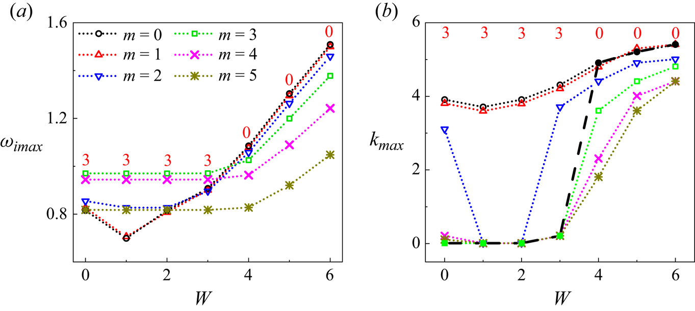
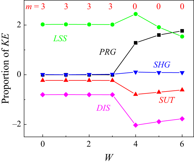
Figure 11 presents the energy budget of the predominant mode as  $W$ gradually changes, in which the predominant modes are indicated by red numbers. Only the results corresponding to the most unstable wavenumber
 $k_{max}$ are given. Similar to figures 7 and 9, the values of
 $LSS$,
 $PRG$ and
 $SHG$ remain positive, while those of
 $SUT$ and
 $DIS$ are negative. It is notable that the term
 $PRG$ is markedly larger than
 $SHG$, especially under large values of
 $W$, indicating that the change of
 $W$ mainly affects the jet instability through gas pressure perturbation instead of shear stress. The physical mechanism lies in that the change of
 $W$ mainly modulates the thickness of the gas velocity boundary layer but does not change the degree of shear stress at the interface. Under relatively low gas velocity (e.g.
 $0\leq W\leq 3$), the change of
 $W$ has little impact on the values of all the energy terms, and the predominant mode remains at
 $m=3$. Once
 $W \ge 3$, the increase of
 $W$ leads to obvious changes of the energy terms
 $LSS$,
 $PRG$,
 $SUT$ and
 $DIS$. Specifically, the value of
 $LSS$ presents an overall decreasing tendency, while the value of
 $PRG$ increases invariably. As the predominant energy term finally changes from
 $LSS$ to
 $PRG$, the enhancement of gas pressure perturbation promotes the transition from helical mode to axisymmetric mode (i.e.
 $m=3$ to 0). For the negative energy terms,
 $DIS$ maintains the smallest value, and thus the viscous dissipation has the primary stabilizing effect.
Energy budget of the most unstable perturbation wave at the predominant mode as  $W$ gradually changes under
 $Re=20.5, Oh=0.41, V_S=0.995, V=3.5, J=0.0013$ and
 $N=1.67\times 10^{-4}$, where the predominant modes are indicated by red numbers.
5. Transition of the predominant modes
As it has been observed in § 4 that the enhancement of the axial shear stress would promote the predominant mode transition to a smaller azimuthal wavenumber  $m$, this section further gives the quantitative measurements on the influence of shear stress through depicting the phase diagrams of different azimuthal modes. In the previous theoretical study of Kubitschek & Weidman (Reference Kubitschek and Weidman2007a), a static rotating liquid column (with constant angular velocity) without axial velocity in a vacuum was considered, in which the effects of Hocking number
 $L$ and
 $Re$ on the predominant mode transition were examined carefully. It is notable that
 $L$ is defined as the reciprocal of
 $We$ which is utilized in this work. A phase diagram of the predominant azimuthal modes in
 $L$–
 $Re$ space is given in their work and the transition boundaries between different modes are identified, as shown by the open symbols in figure 12. As the jet angular velocity increases, the parameters gradually shift from the lower right side to the upper left side of the phase diagram, and the predominant azimuthal mode converts from low
 $m$ to high
 $m$. It is notable that the axial shear stress is totally ignored in their study due to the assumption of a static rotating column. In this section, we further examine the effect of the axial shear stress on mode transition of an axial moving jet through an integration of theoretical analyses and experimental measurements.
Phase diagrams of the azimuthal modes in  $Re$–
 $1/We$ space, where swirling liquid jets in static gas surroundings (
 $W=0$) are considered. The black circles are the results from Kubitschek & Weidman (Reference Kubitschek and Weidman2007a) and the lines denote the results calculated under non-uniform velocity profiles with
 $V_S=0.995$ and
 $V=3.5$;
 $V_S=0.995$ and
 $V=4.5$; and
 $V_S=0.992$ and
 $V=3.5$.

The phase diagram of the predominant azimuthal modes in  $L$–
 $Re$ space under the axial non-uniform velocity profiles described by (2.14) and (2.15) is also given in figure 12. The values of
 $V_S$ and
 $V$ are changed to modulate the strength of axial shear stress. Under the reference state where
 $V=3.5$ and
 $V_S=0.995$, as shown by the red dashed line, it is observed that the mode transitions from
 $m=0$ to
 $2$ and
 $m=1$ to
 $2$ shift to the the upper left direction of the phase diagram comparing with the results of Kubitschek & Weidman (Reference Kubitschek and Weidman2007a), indicating that the mode transitions are delayed and occur at larger angular velocities due to the addition of axial shear stress. However, the mode transitions between the helical modes with larger azimuthal wavenumbers (i.e.
 $m=2$ to 3, 3 to 4 and 4 to 5) would not be affected obviously, which is qualitatively consistent with the previous findings that the azimuthal modes with smaller
 $m$ are affected more markedly by the axial shear effect (see figures 6 and 8). Figure 12 also considers the mode transition boundaries under
 $V=4.5,V_S=0.995$ and
 $V=3.5, V_S=0.992$ (see the blue dotted and green dash-dotted lines, respectively). Comparing with the reference state where
 $V=3.5,V_S=0.995$, these two cases bring in a stronger axial shear stress. It can be observed that the enhanced axial shear stress would cause the mode transitions of
 $m=0$ to 2 and
 $m=1$ to 2 to be further delayed. Moreover, the transitions of helical modes with larger azimuthal wavenumbers would also be delayed with the enhancement of axial shear stress.
To further study the effect of the azimuthal rotation and axial shear flow on the predominant mode transition, the phase diagram of modes  $m=0$–
 $5$ is given in figure 13, considering the variations of
 $Re$ and
 $Re_z$. It is notable that the variation of
 $Re$ under fixed
 $Re_z$
 $(=ReV)$ represents the change of jet angular velocity under constant axial velocity, and the single increase of
 $Re_z$ under fixed
 $Re$ leads to a larger axial velocity, which results in a stronger axial shear stress. Without loss of generality, the value of
 $Re_z$ varies from 0 to 53.58, corresponding to dimensional axial velocities between
 $0$ and
 $1.93\,{\rm m}\,{\rm s}^{-1}$. The theoretical mode boundaries calculated under the non-uniform velocity profile described by (2.14)–(2.15) are depicted in figure 13 by open circles and black solid lines, in which the specific value of
 $V_S=0.985$ is selected to realize a relatively strong axial shear stress. It is clear that our results totally coincide with those of Kubitschek & Weidman (Reference Kubitschek and Weidman2007a) under vanishing axial velocity (i.e.
 $Re_z=0$). At relatively low axial velocity of the jet (e.g.
 $Re_z<34$), the predominant mode will transit from the axisymmetric mode
 $m=0$ to the non-axisymmetric modes
 $m=2$, 3, 4 and 5 step by step as the value of
 $Re$ gradually increases. As the jet axial velocity increases to a relatively high value (e.g.
 $Re_z \ge 34$), the helical mode
 $m=1$ emerges during the mode transition with an increase of
 $Re$. Besides, it can be clearly seen from figure 13 that the increase of
 $Re_z$ has a strong effect on mode transition. For the transition from
 $m=0$ to 2, the transition boundary shifts upward as soon as the value of
 $Re_z$ increases from 0, indicating the delayed mode transition from 0 to 2 even under relatively low axial velocity. The transition boundaries of
 $m=0$ to 1 and
 $m=1$ to 2 also shift upward monotonically with an increase of
 $Re_z$. However, the transition boundary of
 $m=2$–
 $3$ keeps almost unchanged at first as
 $Re_z$ increases. When the value of
 $Re_z$ exceeds 30, the boundary shifts upward dramatically, indicating that the delay of mode transition from 2 to 3 will be triggered under relatively large axial velocity. The transition from
 $m=3$ to
 $m=4$ is found to be delayed apparently if
 $Re_z\ge 40$, whereas the transition from
 $m=4$ to
 $m=5$ is slightly affected by the increase of
 $Re_z$ within the considered range. Therefore, it can be concluded that the enhancement of the axial shear stress leads to the delay of the predominant mode transition from smaller
 $m$ to larger
 $m$, and a more dramatic effect can be observed on the transition between smaller values of
 $m$.
Phase diagrams of the azimuthal modes in  $Re$–
 $Re_z$ space, where the swirling liquid jet in static gas surroundings (
 $W=0$) is considered. The solid lines are theoretical boundaries calculated under non-uniform velocity profiles with
 $V_S=0.985$, and the dashed orange lines are the theoretical boundaries of Kubitschek & Weidman (Reference Kubitschek and Weidman2007a). The coloured squares correspond to the experimental results shown in figure 14.

In order to substantiate the theoretical findings, an experimental study considering the swirling liquid jet in ambient air is also conducted. The experimental facility is able to provide a swirling jet of diameter  $R_1=7$ mm. We select silicone oil for the swirling jet, with physical properties consistent with the reference state in theoretical analysis (i.e.
 $\rho _1=971\, {\rm kg}\,{\rm m}^{-3}$,
 $\mu _1=0.1223\,{\rm Pa}\,{\rm s}$ and
 $\gamma =26\,{\rm mN}\,{\rm m}^{-1}$). A detailed description of the experimental set-up can be found in Appendix D. As the strength of the axial shear stress can be modulated by jet axial velocity, two groups of experiments are conducted (see figure 14), where the jet axial velocities are equal to
 $0.38\,{\rm m}\,{\rm s}^{-1}$ (corresponding to
 $Re_z=10.56$) and
 $1.93\,{\rm m}\,{\rm s}^{-1}$ (corresponding to
 $Re_z=53.58$), respectively. For each axial velocity, the angular velocity
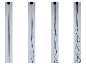
 $\varOmega$ of the swirling jet is increased from an initially very low value to trigger the azimuthal mode transition. Figure 14(a) shows the morphologies of the swirling jet with
 $Re_z=10.56$ under different angular velocities. It can be clearly seen that the azimuthal mode appears to be
 $m=0$, 2 and 3 (from left to right) under
 $\varOmega =47.6$,
 $95.2$ and
 $190.5\,{\rm rad}\,{\rm s}^{-1}$, which correspond to the values of
 $Re=4.63$, 9.26 and 18.52, respectively. It is notable that as the the value of
 $\varOmega$ increases further, the jet cannot form as the flow destabilizes right at the tube exit, which is beyond the scope of the present study. Figure 14(b) displays the images of the swirling jet with
 $Re_z=53.58$ under different angular velocities. The azimuthal mode is
 $m=0$, 2, 3 and 4 (from left to right) when the angular velocity is equal to
 $95.2$,
 $190.5$,
 $224.5$ and
 $275.5\,{\rm rad}\,{\rm s}^{-1}$, corresponding to
 $Re=9.26$, 18.52, 21.83 and 26.78, respectively. It can be clearly seen from figure 14(a,b) that the increase of the rotation leads to the transition of the azimuthal mode from smaller
 $m$ to larger
 $m$, which is consistent with the previous work of Kubitschek & Weidman (Reference Kubitschek and Weidman2007b) and the theoretical findings in the present work. It is important to note that the azimuthal mode of the swirling jet with
 $Re_z=10.56$ is
 $m=2$ when
 $Re=9.26$ (see figure 14a ii), while that of the swirling jet with
 $Re_z=53.58$ appears to be
 $m=0$ (see figure 14b i). Also, the azimuthal mode of the swirling jet with
 $Re_z=10.56$ is
 $m=3$ as
 $Re=18.52$ (see figure 14a iii), whereas that of the swirling jet with
 $Re_z=53.58$ appears to be
 $m=2$ (see figure 14b ii). Since the axial shear stress is strengthened as
 $Re_z$ increases, the above observation suggests that the mode transition will be delayed by the enhancement of the axial shear stress. The experimental results in figure 14 are compared with the previous theoretical findings. As shown in figure 13, the coloured squares represent the experimental settings, with different colours demonstrating different azimuthal modes (red, blue, green, purple correspond to
 $m=0, 2, 3, 4$, respectively). It can be found that the experimental results fall in the range of the theoretical predictions. Therefore, it can be concluded both theoretically and experimentally that the enhancement of the axial shear stress will lead to the delay of the azimuthal mode transition which is triggered by the increase of the angular velocity.
Morphologies of the swirling liquid jet under different axial velocities and angular velocities. (a)  $Re_z=10.56$, corresponding to axial velocity of
 $\bar {U}_1= 0.38\,{\rm m}\,{\rm s}^{-1}$. The azimuthal mode varies as
 $m=0$, 2 and 3 at
 $Re=4.63$, 9.26 and 18.52, corresponding to angular velocity of
 $\varOmega =47.6$,
 $95.2$ and
 $190.5\,{\rm rad}\,{\rm s}^{-1}$, respectively. (b)
 $Re_z=53.58$, corresponding to axial velocity of
 $\bar {U}_1= 1.93\,{\rm m}\,{\rm s}^{-1}$. The azimuthal mode varies as
 $m=0$, 2, 3 and 4 at
 $Re=9.26$, 18.52, 21.83 and 26.78, corresponding to angular velocity of
 $\varOmega =95.2$,
 $190.5$,
 $224.5$ and
 $275.5\,{\rm rad}\,{\rm s}^{-1}$, respectively.

6. Transition of the instability mechanisms
As the transition of predominant mode is related to different instability mechanisms, we also analyse the variation of the primary instability mechanisms according to the energy budget analysis of the predominant mode. In §§ 3 and 4, it has been found that the predominant energy terms with the maximum positive value can be either  $LSS$,
 $SHG$ or
 $PRG$, as shown by figures 5, 7, 9 and 11. We also emphasize that under certain conditions (e.g. at relatively weak axial shear stress and centrifugal force), the term
 $SUT$ can also become the predominant energy term. The typical cases are given in Appendix E. Based on the predominant energy terms, different primary instability mechanisms can be identified. Specifically, the term
 $SUT$ characterizes the instability caused by surface tension, which corresponds to the capillary instability (CPI). Term
 $LSS$ is the direct measurement of the centrifugal force exerted by the swirling jet and thus brings in the centrifugal instability (CTI). The terms
 $SHG$ and
 $PRG$ represent the instability contributed by the axial shear stress and the gas pressure perturbation on the jet interface, respectively, which corresponds to the KHI. As the values of these terms are related to the jet angular velocity, axial velocity and the degree of shear stress represented by the velocity profiles, we consider the transitions of instability mechanisms as the values of
 $Re$,
 $Re_z$ and
 $V_S$ vary.
Figure 15 gives the phase diagrams of primary instability mechanisms in  $Re_z$–
 $Re$ space, which correspond to individual variations of jet axial velocity and angular velocity. The liquid jet evolves in static gas surroundings with
 $W=0$, and different velocity profiles are considered. For the discontinuous velocity profile where
 $V_S=1$, the axial shear effect is ignored, and thus only CPI and CTI exist for the swirling liquid jet, as shown in figure 15(a). It is clearly seen that the primary instability mechanism gradually converts from CPI to CTI with an increase of
 $Re$ (i.e. angular velocity), which is the same as the tendency shown in figure 5. The transition between CPI and CTI occurs around
 $Re \sim O(1)$, and the variation of
 $Re_z$ hardly affects the transition boundary. It is notable that more values of
 $Re$ and
 $Re_z$ than those plotted in figure 15(a) have been calculated to obtain the precise position of transition boundary. The axial shear stress is also taken into account by utilizing the non-uniform velocity profile where
 $V_S<1$. The strength of the axial shear is affected by the values of
 $V_S$ and
 $Re_z$, as has been studied in §§ 4.1 and 4.2. The phase diagrams of instability mechanisms in
 $Re_z$–
 $Re$ space under different values of
 $V_S$
 $(=0.999, 0.996, 0.992)$ are shown in figure 15(b–d). It can be found that the parameter space dominated by KHI is triggered by the axial shear effect. The transition boundaries between KHI and CTI and between KHI and CPI are denoted by the dash-dotted line and dotted line, respectively. For a certain value of
 $V_S$, it can be observed that CPI maintains the primary mechanism at relatively low values of
 $Re_z$ and
 $Re$, indicating that the surface tension dominates the jet instability and the centrifugal and axial shear forces only play a secondary role under relatively low angular and axial velocities of the liquid jet. With an increase of
 $Re$ (i.e. angular velocity), the primary instability mechanism shifts from CPI to CTI, and the critical value of transition remains constant under different values of
 $Re_z$ (i.e. jet axial velocity). The typical cases for the transition of mechanisms from CPI to CTI are also shown clearly in Appendix E. Similarly, the primary instability mechanism converts from CPI to KHI with an increase of
 $Re_z$, and the critical transitional value remains almost constant as
 $Re$ changes. Under relatively large values of
 $Re_z$, it is clear that the increase of
 $Re$ can lead to the transition from KHI to CPI, and the critical transitional value increases with the increase of
 $Re_z$, which indicates that the enhancement of shear stress can delay the transition from KHI to CTI. Comparing the transition boundaries under different values of
 $V_S$, it is observed that a decrease of
 $V_S$ leads to a wider KHI zone and narrower CPI and CTI zones, which also indicates an enhancing effect of axial shear stress on KHI.
Phase diagrams of primary instability mechanisms in  $Re_z$–
 $Re$ space under different velocity profiles: (a)
 $V_S=1$, corresponding to the discontinuous velocity profile, (b)
 $V_S=0.999$, (c)
 $V_S=0.996$ and (d)
 $V_S=0.992$. The CTI mode, KHI mode and CPI mode are denoted by the black squares, red triangles and green diamonds, respectively. The dash-dotted line, dashed line and dotted line denote the boundaries between CTI/KHI mode, CPI/CTI mode and CPI/KHI mode, respectively.

7. Conclusion and outlook
Linear temporal instability analysis of a viscous swirling liquid jet surrounded by ambient gas is carried out, where the importance of axial shear effect on the development of perturbation and transition of azimuthal modes are examined for the first time. The basic flows in azimuthal and axial directions are approximated by the Rankine vortex and the non-uniform velocity profile with the form of parabolic and error functions, respectively. The normal mode method is employed to inspect the perturbation growth of the liquid jet, and the Chebyshev spectral collocation method is utilized to solve the generalized eigenvalue problem. Energy budget analysis is also implemented to reveal the physical mechanism of jet instability. The effect of azimuthal rotation on jet instability is firstly studied through changing the angular velocity of the jet (non-dimensionalized by  $Re$) under constant jet axial velocity (non-dimensionalized by
 $Re_z$). It is found that the enhancement of the rotation has a dual effect on the axisymmetric mode but promotes the instability of the helical modes. Moreover, the predominant mode gradually converts to the mode with the larger azimuthal wavenumber
 $m$ with an increase of
 $Re$. The energy budget analysis shows that the shear stress and the perturbation pressure exerted by the ambient gas contribute to the axisymmetric mode, while the helical modes are mainly induced by the centrifugal force. The effects of the axial shear flow on jet instability are examined, in which the variations of jet surface velocity
 $V_S$, axial average velocity
 $V$ and ambient gas velocity
 $W$ are each considered. A decrease of
 $V_S$ could enhance the axial shear stress of the jet, thus promoting the jet instability under different azimuthal wavenumbers
 $m$ and leading to the transition of predominant mode to smaller
 $m$. The energy budget analysis indicates that the shear stress and the gas pressure perturbation play a more significant role over the centrifugal force under relatively low
 $V_S$. The increase of
 $V$ also enhances the axial shear stress of the jet. Therefore, the variation characteristics of jet instability with the increase of
 $V$ are similar to those as
 $V_S$ decreases. As the value of
 $W$ gradually diverges from 1, the jet instability would be enhanced and the predominant mode converts to the azimuthal mode with smaller
 $m$. The energy budget shows that the jet instability is mainly induced by gas pressure perturbation as the variation of
 $W$ changes the thickness of gas velocity boundary layer but does not affect the shear stress. The effect of the axial shear stress is further analysed by comparing our results with those in Kubitschek & Weidman (Reference Kubitschek and Weidman2007a) where the instability of a swirling liquid column in a vacuum without axial flow was studied. It is found that the axial shear stress can delay the mode transition obviously, especially under small azimuthal wavenumber
 $m$. Experimental studies under different jet axial velocities are further carried out, which find that a jet with higher axial velocity exhibits the azimuthal mode with smaller
 $m$ under a fixed angular velocity, thus substantiating the findings of the theoretical work. Three instability mechanisms are identified according to the energy budget analysis, i.e. the CPI, the CTI and the KHI. The effects of azimuthal rotation and axial flow on the transition of instability mechanisms are examined by phase diagrams in
 $Re_z$–
 $Re$ space, where different values of
 $V_S$ are considered. This work is expected to provide some guidances for understanding the physical mechanisms of the instability of a swirling liquid jet, contributing to process optimization in real applications such as liquid atomization and combustion.
At the end of this paper, some possible avenues for future work are provided and discussed, as presented in the following subsections.
7.1. Spatiotemporal instability analysis
The current work is under the scope of convective temporal instability, which is confirmed to be feasible as the swirling liquid jets establish downstream after flowing out of the rotating tube. However, for certain parametric space (e.g. very low axial jet velocity), the swirling liquid jets fail to be generated, resulting in the disintegration of liquid interface to droplets right at the tube exit. From the theoretical perspective, this behaviour corresponds to the AI, where the initial disturbances at the jet interface propagate both upstream and downstream. Therefore, it is of great significance to further study the spatiotemporal instability of the jets, which contributes to clarifying the criterion of the formation of swirling liquid jets. Once the jets fall within the parametric space of CI, the spatial analysis of jet instability can also be carried out, which is intended to present the evolutive characteristics of disturbances in space more clearly. More details of the discussions of the spatiotemporal instability and the spatial instability can be found in Appendix F.
7.2. Global instability analysis
In the present theoretical model, the effect of gravity is ignored as we mainly focus on the development of disturbances at the early stages of jet evolution. Therefore, only the local instability of swirling jets is considered, where the radius of the jet is assumed to be spatially invariant. However, the gravity force could play a more prominent effect as the jet evolves further downstream, and the radius of the jet is considered to be spatially relevant in real situations. To figure out the effect of gravity, a global instability analysis is desired, which takes the gravity force and the variation of the jet radius into account.
7.3. Swirling instability of non-Newtonian liquid jets
Non-Newtonian liquids commonly occur in engineering applications, such as gelled propellants and slurries. Compared with a Newtonian liquid whose shear stress is proportional to the shear rate, a non-Newtonian liquid exhibits abundant rheological behaviours due to existence of complex microstructures (Phan-Thien & Mai-Duy Reference Phan-Thien and Mai-Duy2013; Ewoldt & Saengow Reference Ewoldt and Saengow2022). The axisymmetric instability characteristics of a non-Newtonian liquid jet have been proved to be quite different from those of a Newtonian jet (Mohamed et al. Reference Mohamed, Herrada, Gañán Calvo and Montanero2015; Ding et al. Reference Ding, Mu, Si and Jian2022; Mousavi, Siavashi & Bagheri Reference Mousavi, Siavashi and Bagheri2023). However, systematic analysis of the circumferential instability of non-Newtonian swirling jets is still limited, which would be our future work.
Acknowledgements
The authors gratefully acknowledge the anonymous reviewers for offering significant suggestions to facilitate the improvement of the paper.
Funding
This work was supported by the National Natural Science Foundation of China (grant nos. 12272372, 12027801 and 12388101), Youth Innovation Promotion Association CAS (nos. 2018491 and 2023477), Chinese Academy of Sciences Project for Young Scientists in Basic Research (YSBR-087) and USTC Research Funds of the Double First-Class Initiative (YD2090002020).
Declaration of interests
The authors report no conflict of interest.
Appendix A. Derivation of the axial velocity profiles
To derive the analytical axial velocity profiles of the liquid jet and the gas surroundings, we consider the axisymmetric axial flow, represented by  $\boldsymbol {U}_i=U_i(r)\boldsymbol {e}_z$, where
 $i = 1, 2$ represent the liquid and gas phases, respectively.
For the liquid jet, (2.2) can be reduced to
 \begin{equation} \frac{1}{r}\frac{{\rm d}}{{\rm d}r}\left[r\frac{{\rm d}U_1(r)}{{\rm d}r}\right]={-}\frac{G}{\mu_1}, \end{equation}
where  $G=-\partial p_1/\partial z$ is the adverse pressure gradient. The general solution of (A1) is
 \begin{equation} U_1(r)={-}\frac{G}{4\mu_1}r^2+B\ln r+C. \end{equation}
Considering the boundary condition at the axis (i.e. (2.3)), the value of  $B$ must be equal to 0. Assuming the axial velocity at the interface (
 $r=R_1$) to be
 $U_S$, we have
 \begin{equation} C=U_S+\frac{GR_1^2}{4\mu_1}. \end{equation}
Since the flow rate of the liquid jet can be expressed as
 \begin{equation} Q=\int_0^{2{\rm \pi}}\,{\rm d}\theta\int_0^{R_1}U_1(r)r\,{\rm d}r={\rm \pi}\left[U_SR_1^2+\frac{GR_1^4}{8\mu_1}\right], \end{equation}
the basic axial velocity profile of the liquid jet can be obtained as
 \begin{equation} U_1^*(r)=U_S+2\left[U_S-\frac{Q}{{\rm \pi} R_1^2}\right]\left[\frac{r^2}{R_1^2}-1\right], \end{equation}
which corresponds to (2.12) in the main text.
The basic velocity profile of the gas surroundings is assumed with the form  $U_2(r)=a{\rm {erf}}[b(r-R_1)]+c$, where
 ${\rm {erf}}(x)$ is the error function and can be expressed as
 ${\rm {erf}}(x) = 2/\sqrt {{\rm \pi} }\int _0^x {\rm e}^{-\eta ^2}\,{\rm d}\eta$. As the axial velocity at infinity (
 $r\rightarrow \infty$) is equal to
 $U_\infty$, we have
 \begin{equation} a+c=U_\infty. \end{equation}
Taking the basic velocity profile into the boundary conditions of (2.4) and (2.6), we can obtain the following equations:
 \begin{gather} c=U_S, \end{gather}
 \begin{gather} \frac{2\mu_2 ab}{\sqrt{\rm \pi}}=\frac{4\mu_1}{R_1}\left[U_S-\frac{Q}{{\rm \pi} R_1^2}\right]. \end{gather}
Combining (A6)–(A8), the expression of  $a, b$ and
 $c$ can be determined. Finally, the basic velocity profile of the gas surroundings can be obtained as
 \begin{equation} U_2(r)=(U_\infty-U_S){\rm{erf}}\left[\frac{\sqrt{\rm \pi}}{2}\frac{4\mu_1(U_S-Q/{\rm \pi} R_1^2)}{\mu_2(U_\infty-U_S)}\left(\frac{r}{R_1}-1\right)\right]+U_S, \end{equation}
which corresponds to (2.13) in the main text.
Appendix B. Validations of numerical calculation
To validate the numerical calculation, a convergence study of the calculated complex frequency  $\omega$ (
 $=\omega _r+{\rm i}\omega _i$) is firstly carried out, considering different numbers of the collocation points (
 $N_1$ and
 $N_2$) and variations of the radius ratio
 $a$. The results are given in tables 1 and 2, respectively, which indicate that a selection of values
 $N_1 \ge 20$,
 $N_2 \ge 50$ and
 $a \ge 8$ is sufficient to ensure numerical convergence. Therefore, we choose
 $N_1=30$,
 $N_2=60$ and
 $a=10$ in all our calculations.
Calculated complex frequency  $\omega$ (
 $=\omega _r + {\rm i} \omega _i$) under different values of
 $N_1$ and
 $N_2$, where
 $Re=20.5, We=71.3, V_S=0.995, W=0, V=3.5, J=0.0013, N=1.67\times 10^{-4}, m=3, k=1$ and
 $a=10$.

Calculated complex frequency  $\omega$ (
 $=\omega _r+{\rm i}\omega _i$) under different values of
 $a$, where
 $Re=20.5, We=71.3, V_S=0.995, W=0, V=3.5, J=0.0013, N=1.67\times 10^{-4}, m=3, k=1, N_1=30$ and
 $N_2=60$.

To check the accuracy of our code, we further simplify the current model and compare the calculated results with those of previous studies. On the one hand, the model can be reduced to a non-swirling liquid jet in co-flowing gas stream by setting  $Re= 0$ and
 $We=0$. In this way, the circumferential velocity profile is ignored, and the axial velocity profile is set to be consistent with our previous work, where the hyperbolic-tangent function is utilized to approximate the basic flows (Si et al. Reference Si, Li, Yin and Yin2009). The comparison between the current results and those of Si et al. (Reference Si, Li, Yin and Yin2009) is given in figure 16(a), where the perturbation growth rates of axisymmetric mode with
 $m=0$ are considered under the same axial Reynolds number and Ohnesorge number. Clearly, a good agreement can be reached. On the other hand, the swirling liquid jet can be reduced to a swirling column without axial velocity by setting
 $V=W=0$. The presence of gas surroundings is totally ignored by setting
 $J=N=0$. By further ignoring the azimuthal velocity of the gas phase and only considering the rotation of the liquid jet, our model can be simplified to that considered by Kubitschek & Weidman (Reference Kubitschek and Weidman2007a). Figure 16(b) shows the growth rate curve of our calculation and that in Kubitschek & Weidman (Reference Kubitschek and Weidman2007a) for the helical mode with
 $m=1$, under the same Reynolds and Weber numbers. A good agreement can also be reached.
Validations of our numerical code with previous studies. (a) Non-swirling axisymmetric liquid jet in co-flowing gas stream, where  $Re_z=100, Oh=3.16\times 10^{-3}, J=0.0013, N=0.018$ and
 $m=0$. The basic velocity profile is unified as the hyperbolic-tangent function and the results are compared with those of Si et al. (Reference Si, Li, Yin and Yin2009). (b) Swirling liquid column in a vacuum, where
 $Re=10, We=100, V=0, V_{S}=1, W=0, J=0, N=0$ and
 $m=1$. Our results are compared with those of Kubitschek & Weidman (Reference Kubitschek and Weidman2007a).

Appendix C. Specific forms of the terms in energy budget analysis
 \begin{gather} \overline{KE}=\frac{1}{2T\lambda}\int_0^T\int_0^\lambda\int_0^{2{\rm \pi}}\int_0^1\left(\frac{\partial}{\partial t}+U_1\frac{\partial}{\partial z}+W_1\frac{\partial}{r\partial\theta}\right)(\tilde{u}_1^2+\tilde{v}_1^2+\tilde{w}_1^2)r\,{\rm d}r\,{\rm d}\theta \,{\rm d}z\,{\rm d}t, \end{gather}
 \begin{gather}\overline{REY}={-}\frac{1}{T\lambda}\int_0^T\int_0^\lambda\int_0^{2{\rm \pi}}\int_0^1\left(\tilde{u}_1\tilde{v}_1\frac{{\rm d}U_1}{{\rm d}r}+\tilde{w}_1\tilde{v}_1\frac{{\rm d}W_1}{{\rm d}r}-\tilde{w}_1\tilde{v}_1\frac{W_1}{r}\right)r\,{\rm d}r\,{\rm d}\theta \,{\rm d}z\,{\rm d}t, \end{gather}
 \begin{gather}\overline{PRL}={-}\frac{1}{T\lambda}\int_0^T\int_0^{2{\rm \pi}}\int_0^1[\tilde{p}_1\tilde{u}_1]_{z=0}^{z=\lambda}r\,{\rm d}r\,{\rm d}\theta\,{\rm d}t, \end{gather}
 \begin{gather}\overline{PRG}={-}\frac{1}{T\lambda}\int_0^T\int_0^{2{\rm \pi}}\int_0^\lambda[\tilde{p}_2\tilde{v}_1]_{r=1}\,{\rm d}z\,{\rm d}\theta \,{\rm d}t, \end{gather}
 \begin{gather}\overline{LSS}=\frac{1}{T\lambda}\int_0^T\int_0^{2{\rm \pi}}\int_0^{\lambda}\left[\frac{W_1^2}{r}\eta\tilde{v}_1\right]_{r=1}\,{\rm d}z\,{\rm d}\theta \,{\rm d}t, \end{gather}
 \begin{gather}\overline{OGS}={-}\frac{1}{T\lambda}\int_0^T\int_0^{2{\rm \pi}}\int_0^{\lambda}\left[J\frac{W_2^2}{r}\eta\tilde{v}_1\right]_{r=1}\,{\rm d}z\,{\rm d}\theta \,{\rm d}t, \end{gather}
 \begin{gather}\overline{NVG}=\frac{2N}{T\lambda Re}\int_0^T\int_0^{2{\rm \pi}}\int_0^{\lambda}\left[\frac{\partial\tilde{v}_2}{\partial r}\tilde{v}_1\right]_{r=1}\,{\rm d}z\,{\rm d}\theta\,{\rm d}t, \end{gather}
 \begin{gather}\overline{SUT}=\frac{1}{WeT\lambda}\int_0^T\int_0^{2{\rm \pi}}\int_0^\lambda\left[\left(1+\frac{\partial^2}{\partial\theta^2}+\frac{\partial^2}{\partial z^2}\right)\eta\tilde{v}_1\right]_{r=1}\,{\rm d}z \,{\rm d}\theta\,{\rm d}t, \end{gather}
 \begin{gather}\overline{SHL}=\frac{1}{T\lambda Re}\int_0^T\int_0^{2{\rm \pi}}\int_0^1\left[\tilde{v}_1\left(\frac{\partial\tilde{v}_1}{\partial z}+\frac{\partial\tilde{u}_1}{\partial r}\right)+\tilde{w}_1\left(\frac{\partial\tilde{w}_1}{\partial z}+\frac{\partial\tilde{u}_1}{r\partial\theta}\right)\right]_{z=0}^{z=\lambda}r\,{\rm d}r\,{\rm d}\theta \,{\rm d}t, \end{gather}
 \begin{gather}\overline{NVL}=\frac{1}{T\lambda Re}\int_0^T\int_0^{2{\rm \pi}}\int_0^1\left[2\tilde{u}_1\frac{\partial\tilde{u}_1}{\partial z}\right]_{z=0}^{z=\lambda}r\,{\rm d}r\,{\rm d}\theta\,{\rm d}t, \end{gather}
 \begin{gather}\overline{SHG}=\frac{1}{T\lambda Re}\int_0^T\int_0^{2{\rm \pi}}\int_0^\lambda\left[N\tilde{u}_1\left(\frac{\partial\tilde{u}_2}{\partial r}+\frac{\partial\tilde{v}_2}{\partial z}\right)\right]_{r=1}\,{\rm d}z\,{\rm d}\theta\,{\rm d}t, \end{gather}
 \begin{gather}\overline{SHB}=\frac{1}{T\lambda Re}\int_0^T\int_0^{2{\rm \pi}}\int_0^\lambda\left[\eta\left(N\frac{{\rm d}^2U_2}{{\rm d}r^2}-\frac{{\rm d}^2U_1}{{\rm d}r^2}\right)\tilde{u}_1\right]_{r=1}\,{\rm d}z\,{\rm d}\theta \,{\rm d}t, \end{gather}
 \begin{gather}\overline{AHG}=\frac{1}{T\lambda Re}\int_0^T\int_0^{2{\rm \pi}}\int_0^\lambda\left[N\tilde{w}_1\left(\frac{\partial\tilde{v}_2}{\partial\theta}+\frac{\partial\tilde{w}_2}{\partial r}-\tilde{w}_2\right)\right]_{r=1}\,{\rm d}z\,{\rm d}\theta\,{\rm d}t, \end{gather}
 \begin{gather}\overline{AHB}=\frac{1}{T\lambda Re}\int_0^T\int_0^{2{\rm \pi}}\int_0^\lambda\left\{\tilde{w}_1\eta\left[N\left(\frac{{\rm d}^2W_2}{{\rm d}r^2}+W_2-\frac{{\rm d}W_2}{{\rm d}r}\right)\right.\right.\nonumber\\ \left.\left.-\left(\frac{{\rm d}^2W_1}{{\rm d}r^2}+W_1-\frac{{\rm d}W_1}{{\rm d}r}\right)\right]\right\}_{r=1}\,{\rm d}z\,{\rm d}\theta \,{\rm d}t, \end{gather}
 \begin{gather}\overline{DIS}={-}\frac{1}{T\lambda Re}\int_0^T\int_0^\lambda\int_0^{2{\rm \pi}}\int_0^1\left[2\left(\frac{\partial\tilde{v}_1}{\partial r}\right)^2+2\left(\frac{\partial\tilde{w}_1}{r\partial\theta}+\frac{\tilde{v}_1}{r}\right)^2+2\left(\frac{\partial\tilde{u}_1}{\partial z}\right)^2\right.\nonumber\\ \left.+\left(\frac{\partial\tilde{w}_1}{\partial r}+\frac{\partial\tilde{v}_1}{r\partial\theta}-\frac{\tilde{w}_1}{r}\right)^2+\left(\frac{\partial\tilde{v}_1}{\partial z}+\frac{\partial\tilde{u}_1}{\partial r}\right)^2+\left(\frac{\partial\tilde{u}_1}{r\partial\theta}+\frac{\partial\tilde{w}_1}{\partial z}\right)^2\right]r\,{\rm d}r\,{\rm d}\theta\,{\rm d}z\,{\rm d}t. \end{gather}
Appendix D. Set-up of experiments
The experimental platform for generating the swirling liquid jet is shown in figure 17. The liquid jet is generated from a 30 cm long rotating tube with an inner diameter of 7 mm, which is supported by the rotary fitting. A DC motor, coupled with a transmission gear with a diameter ratio of  $7:10$, provides the angular velocity of the rotating tube up to
 $272\,{\rm rad}\,{\rm s}^{-1}$. The liquid is supplied from the reservoir connected to the top of the rotating tube, and the actuating pressure of liquid is created by a nitrogen cylinder which is able to produce an axial jet velocity of up to
 $2\,{\rm m}\,{\rm s}^{-1}$ at the tube exit. The liquid is recycled by a tank positioned 1 m below the outlet of the tube. A high-speed camera (Phantom V2012) operating at 4000 frames per second is used to capture the interface morphology of the swirling jet on side views.
Schematic of the experimental platform.

To confirm that the rotation of the liquid jet is fully developed inside the tube, we compare the angular velocity of the swirling jet (i.e.  $\varOmega$) measured at the tube exit with the angular velocity of the rotating tube (i.e.
 $\varOmega _{t}$), and the results are shown in figure 18. It can be clearly seen that the relationship between
 $\varOmega _m$ and
 $\varOmega _{t}$ satisfies
 $\varOmega =\varOmega _{t}$, as indicated by the red dashed line. The results suggest that the angular velocity of the jet has been fully developed inside the tube.
Measured angular velocities of the swirling jet ( $\varOmega$) under different angular velocities of the rotating tube (
 $\varOmega _{t}$). The relationship between
 $\varOmega$ and
 $\varOmega _{t}$ satisfies
 $\varOmega =\varOmega _{t}$ (the red dashed line).

Appendix E. Energy budget analysis under low axial shear stress
The energy budget analysis of the effect of rotation with relatively low axial shear stress ( $V_S=0.999$,
 $Re_z=20$) is given in this appendix. Figure 19 shows the energy budget of the most unstable axial wavenumber at the predominant mode as
 $Re$ varies, in which all the energy terms are divided by
 $KE$ to measure the proportion of each term on the changing rate of the disturbance kinetic energy. It should be noted that the terms
 $REY, NVG, AHG, SHB,\ AHB$ and
 $OGS$ are not shown in the figure since their values are less than 5 % of
 $KE$. Under relatively low
 $Re$ (e.g.
 $Re<2$), the surface tension mainly contributes to jet instability as the term
 $SUT$ has the largest positive value, thus promoting the axisymmetric instability (i.e.
 $m=0$) of the swirling jet under weak rotation. As
 $Re$ increases, the value of
 $SUT$ decreases and eventually becomes negative, indicating that the surface tension plays a stabilizing effect. Meanwhile, the value of
 $LSS$ increases over
 $SUT$ and remains as the largest term, indicating that the centrifugal force becomes the predominant factor for jet instability. With a continuing increase of
 $Re$, the helical modes with
 $m\ge 2$ are triggered under the dominance of the centrifugal force. As for the negative terms which suppress the jet instability, the viscous dissipation effect plays the primary stabilizing role as
 $DIS$ has the smallest negative values.
Energy budget of the most unstable perturbation wave at the predominant mode as  $Re$ changes under
 $Oh=0.41, Re_z=20, V_S=0.999, W=0, J=0.0013$ and
 $N=1.67\times 10^{-4}$, where the predominant modes are indicated by red numbers.

Appendix F. Further discussions about convective versus absolute instability and temporal versus spatial analysis
It is well known that the AI mechanism exists for the instability of liquid jets. However, for the swirling liquid jets considered in this work, the jets maintain CI, which can be proved by a spatiotemporal instability analysis. Different from the temporal instability analysis where a real axial wavenumber  $k$ and a complex perturbation frequency
 $\omega$ are assumed, the spatiotemporal instability analysis considers the complex axial wavenumber
 $k$ and perturbation frequency
 $\omega$ (i.e.
 $k=k_r+{\rm {i}}k_i$ and
 $\omega =\omega _r+{\rm {i}}\omega _i$, respectively). The AI and CI characteristics of the liquid jet can be determined from the solutions of the dispersion relation
 $D(\omega, m, k; Re, We, V_S, V, W, J, N)=0$ which have zero group velocity, namely for the complex pair (
 $k_0,\,\omega _0$):
 \begin{equation} \frac{\partial\omega}{\partial k}|_{k_0}=0,\quad \omega_0=\omega(k_0, m;Re, We, V_S, V, W, J, N). \end{equation}
In general, there are two distinct spatial branches of solutions of  $D=0$ on the complex
 $k$ plane. The two branches will approach each other as the growth rate
 $\omega _i$ is decreased from large positive values, and a saddle point on the complex
 $k$ plane will occur at point
 $k=k_0$. It is notable that the physical saddle point must satisfy the Briggs–Bers collision criterion (Briggs Reference Briggs1964; Bers Reference Bers1973; Huerre & Rossi Reference Huerre and Rossi1998). According to the Briggs–Bers collision criterion, the only relevant complex pair (
 $k_0, \omega _0$) is the physical one if two branches come respectively from the downstream-propagating branch
 $k^+(\omega )$ and upstream-propagating branch
 $k^-(\omega )$ on the complex
 $k$ plane. At the saddle point, if
 $\omega _{0i}<0$, the flow is considered to be convective unstable, while if
 $\omega _{0i}>0$, the flow is said to be absolute unstable. For the swirling liquid jet considered in our study, the isopotential line of
 $\omega _i$ and the saddle point on the complex
 $k$ plane under the reference state are given in figure 20. It is notable that only the saddle point under the azimuthal mode
 $m=3$ is depicted as it acts as the predominant mode. The saddle point at
 $k_0=(0.24, -0.50)$ satisfies the Briggs–Bers collision criterion, with the corresponding value of
 $\omega _{0i}=-0.0071$, indicating that the swirling liquid jet is dominated by CI.
Isopotential lines of  $\omega _i$ and the saddle point (
 $k_{0r}=0.24, k_{0i}=-0.5, \omega _{0i}=-0.0071$) on the complex
 $k$ plane for azimuthal mode
 $m=3$ under the reference state (
 $Re=20.5, We=71.3, V_S=0.995, V=3.5, W=0, J=0.0013$ and
 $N=1.67\times 10^{-4}$).

As it has been confirmed that the evolution of the jet is decided by CI, this work considers the temporal instability of disturbances. It should be noted that for the liquid jet with axial downstream velocity, a spatial framework may be more relevant to applications. However, it has been proved that the spatial growth rate of perturbation can be converted to the temporal one and vice versa through the Gaster transformation (Gaster Reference Gaster1962), which has been widely utilized in various researches (Schmid & Henningson Reference Schmid and Henningson2001; Jia et al. Reference Jia, Xie, Deng, He, Yang and Fu2023; Mohamed, Sesterhenn & Biancofiore Reference Mohamed, Sesterhenn and Biancofiore2023). Considering that the spatial instability analysis is mathematically much more challenging than the temporal one, we select the temporal instability analysis for our theoretical model. We further emphasize that in our temporal instability analysis, it has been found that the dimensionless phase velocity for the propagation of disturbance approaches the jet axial velocity (see figure 2 and the corresponding discussion). Therefore, the disturbance only grows temporally and hardly propagates upstream or downstream of the jet under the local framework along the jet, which proves the rationality of the temporal instability analysis.



