1 Introduction
The Reynolds-stress tensor
 $-\unicode[STIX]{x1D70C}\unicode[STIX]{x1D633}_{ij}$
(where
 $\unicode[STIX]{x1D633}_{ij}:=\overline{u_{i}^{\prime }u_{j}^{\prime }}$
are the second-moments of the fluctuating velocity components,
 $u_{i}\in \{u,v,w\}$
are the velocity components in a Cartesian reference frame
 $x_{i}\in \{x,y,z\}$
,
 $\overline{(\cdot )}$
denotes Reynolds (ensemble) averaging and
 $(\cdot )^{\prime }$
turbulent fluctuations around the mean value) represents the influence of turbulent momentum-mixing on the mean flow (Pope Reference Pope2000, pp. 86–87). Throughout the paper we consider incompressible flow (with density
 $\unicode[STIX]{x1D70C}\approxeq \text{const.}$
), in an inertial reference frame (Speziale Reference Speziale1989), with a Newtonian constitutive relation for the viscous stresses (Davidson Reference Davidson2004, (2.4), p. 31), and we assume that the variations of dynamic viscosity are negligible (
 $\unicode[STIX]{x1D707}\approxeq \text{const.}$
). The exact equation for the transport of
 $\unicode[STIX]{x1D633}_{ij}$
(Pope Reference Pope2000, 7.178–7.181, p. 315)
 $$\begin{eqnarray}\displaystyle \underbrace{\unicode[STIX]{x1D70C}\frac{\unicode[STIX]{x2202}\overline{u_{i}^{\prime }u_{j}^{\prime }}}{\unicode[STIX]{x2202}t}+\unicode[STIX]{x1D70C}\bar{u}_{\ell }\frac{\unicode[STIX]{x2202}\overline{u_{i}^{\prime }u_{j}^{\prime }}}{\unicode[STIX]{x2202}x_{\ell }}}_{C_{ij}} & = & \displaystyle \underbrace{\frac{\unicode[STIX]{x2202}}{\unicode[STIX]{x2202}x_{\ell }}\left(\unicode[STIX]{x1D707}\frac{\unicode[STIX]{x2202}\overline{u_{i}^{\prime }u_{j}^{\prime }}}{\unicode[STIX]{x2202}x_{\ell }}\right)}_{d_{ij}^{(\unicode[STIX]{x1D707})}}+\underbrace{\frac{\unicode[STIX]{x2202}}{\unicode[STIX]{x2202}x_{\ell }}(-\unicode[STIX]{x1D70C}\overline{u_{i}^{\prime }u_{j}^{\prime }u_{\ell }^{\prime }})}_{d_{ij}^{(u)}}+\underbrace{\left(-\overline{u_{i}^{\prime }\frac{\unicode[STIX]{x2202}p^{\prime }}{\unicode[STIX]{x2202}x_{j}}}-\overline{u_{j}^{\prime }\frac{\unicode[STIX]{x2202}p^{\prime }}{\unicode[STIX]{x2202}x_{i}}}\right)}_{\unicode[STIX]{x1D6F1}_{ij}}\nonumber\\ \displaystyle & & \displaystyle +\,\underbrace{\left(-\unicode[STIX]{x1D70C}\overline{u_{i}^{\prime }u_{\ell }^{\prime }}\frac{\unicode[STIX]{x2202}\bar{u}_{j}}{\unicode[STIX]{x2202}x_{\ell }}-\unicode[STIX]{x1D70C}\overline{u_{j}^{\prime }u_{\ell }^{\prime }}\frac{\unicode[STIX]{x2202}\bar{u}_{i}}{\unicode[STIX]{x2202}x_{\ell }}\right)}_{P_{ij}}-\underbrace{\left(2\unicode[STIX]{x1D707}\overline{\frac{\unicode[STIX]{x2202}u_{i}^{\prime }}{\unicode[STIX]{x2202}x_{\ell }}\frac{\unicode[STIX]{x2202}u_{j}^{\prime }}{\unicode[STIX]{x2202}x_{\ell }}}\right)}_{\unicode[STIX]{x1D70C}\unicode[STIX]{x1D700}_{ij}}\end{eqnarray}$$
states that the convection of
 $\unicode[STIX]{x1D633}_{ij}$
by the mean velocity field
 $C_{ij}$
is the balance of five mechanisms: diffusion by molecular viscosity
 $d_{ij}^{(\unicode[STIX]{x1D707})}$
, diffusion by the fluctuating velocity field
 $d_{ij}^{(u)}$
, interaction of the fluctuating velocity with the fluctuating pressure gradient
 $\unicode[STIX]{x1D6F1}_{ij}$
, production by the interaction of the Reynolds stresses with mean velocity gradients
 $P_{ij}$
and destruction by molecular friction
 $-\unicode[STIX]{x1D70C}\unicode[STIX]{x1D700}_{ij}$
. Notice that deterministic body forces (e.g. gravity in incompressible flow) do not appear in (1.1) (i.e. do not influence directly
 $\unicode[STIX]{x1D633}_{ij}$
). Budgets of (1.1) in wall turbulence have been studied via DNS (Kim Reference Kim2012) by various authors, for plane channel (Mansour, Kim & Moin Reference Mansour, Kim and Moin1988; Moser, Kim & Mansour Reference Moser, Kim and Mansour1999), pipe (Khoury et al.
Reference Khoury, Schlatter, Noorani, Fischer, Brethouwer and Johansson2013) or boundary-layer (Sillero, Jiménez & Moser Reference Sillero, Jiménez and Moser2013) flows. On the other hand, although the dissipation tensor
 $$\begin{eqnarray}\displaystyle \unicode[STIX]{x1D700}_{ij}:=2\unicode[STIX]{x1D708}\overline{\frac{\unicode[STIX]{x2202}u_{i}^{\prime }}{\unicode[STIX]{x2202}x_{\ell }}\frac{\unicode[STIX]{x2202}u_{j}^{\prime }}{\unicode[STIX]{x2202}x_{\ell }}} & & \displaystyle\end{eqnarray}$$
has been examined (Mansour et al.
Reference Mansour, Kim and Moin1988) as part of the budgets of (1.1), and with respect to its anisotropy (Lai & So Reference Lai and So1990; Jovanović, Ye & Durst Reference Jovanović, Ye and Durst1995), to the authors knowledge, the transport equations for
 $\unicode[STIX]{x1D700}_{ij}$
in wall turbulence have not been studied in detail. Instead, attention has concentrated on its half-trace
 $$\begin{eqnarray}\displaystyle \unicode[STIX]{x1D700}:=\frac{1}{2}\unicode[STIX]{x1D700}_{mm}\stackrel{(1.2a)}{=}\unicode[STIX]{x1D708}\overline{\frac{\unicode[STIX]{x2202}u_{m}^{\prime }}{\unicode[STIX]{x2202}x_{\ell }}\frac{\unicode[STIX]{x2202}u_{m}^{\prime }}{\unicode[STIX]{x2202}x_{\ell }}}>0, & & \displaystyle\end{eqnarray}$$
which represents the dissipation rate of the turbulent kinetic energy
 $k:=(r_{mm})/2$
and is strictly positive being the average of a sum of squares of real numbers (Schumann Reference Schumann1977). In (1.2)
 $\unicode[STIX]{x1D708}:=\unicode[STIX]{x1D70C}^{-1}\unicode[STIX]{x1D707}$
is the kinematic viscosity. Notice that although most authors (Mansour et al.
Reference Mansour, Kim and Moin1988; Lai & So Reference Lai and So1990; Speziale & Gatski Reference Speziale and Gatski1997; Moser et al.
Reference Moser, Kim and Mansour1999; Pope Reference Pope2000; Jakirlić & Hanjalić Reference Jakirlić and Hanjalić2002; Hoyas & Jiménez Reference Hoyas and Jiménez2008) use definition (1.2a
) for
 $\unicode[STIX]{x1D700}_{ij}$
, there are some workers in the field (Jovanović et al.
Reference Jovanović, Ye and Durst1995; Oberlack Reference Oberlack1997) who do not include the factor
 $2$
in (1.2a
), with corresponding absence of the factor
 $1/2$
in (1.2b
).
In an important early work, Lee & Reynolds (Reference Lee, Reynolds, Durst, Launder, Lumley, Schmidt and Whitelaw1987) analysed their DNS computations of homogeneous turbulence (distorted by different types of strain and at different non-dimensional mean strain rates
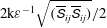 $2\text{k}\unicode[STIX]{x1D700}^{-1}\sqrt{(\overline{\unicode[STIX]{x1D61A}}_{ij}\overline{\unicode[STIX]{x1D61A}}_{ij})}/2$
and then left unstrained to relax) using AIM (anisotropy invariant mapping) of the second-moment tensors of the fluctuating fields of velocity
 $\unicode[STIX]{x1D633}_{ij}:=\overline{u_{i}^{\prime }u_{j}^{\prime }}$
, dissipation
 $\unicode[STIX]{x1D700}_{ij}$
(1.2b
) and vorticity (Davidson Reference Davidson2004,
 $\unicode[STIX]{x1D74E}:=\text{rot}\,\boldsymbol{V}$
, pp. 39–50)
 $\overline{\unicode[STIX]{x1D714}_{i}^{\prime }\unicode[STIX]{x1D714}_{j}^{\prime }}$
, with the underlying idea that
 $\overline{u_{i}^{\prime }u_{j}^{\prime }}$
characterizes the anisotropy of the large structures whereas
 $\unicode[STIX]{x1D700}_{ij}$
and
 $\overline{\unicode[STIX]{x1D714}_{i}^{\prime }\unicode[STIX]{x1D714}_{j}^{\prime }}$
measure the anisotropy of the small scales. They concluded that in the distortion phase ‘the vorticity field
 $\overline{\unicode[STIX]{x1D714}_{i}^{\prime }\unicode[STIX]{x1D714}_{j}^{\prime }}$
is always more anisotropic than the velocity field
 $\overline{u_{i}^{\prime }u_{j}^{\prime }}$
’ (Lee & Reynolds Reference Lee, Reynolds, Durst, Launder, Lumley, Schmidt and Whitelaw1987, p. 60) and that in the relaxation phase ‘the large-scale anisotropy is also coupled with the small-scale turbulence’ (Lee & Reynolds Reference Lee, Reynolds, Durst, Launder, Lumley, Schmidt and Whitelaw1987, p. 66). Durbin & Speziale (Reference Durbin and Speziale1991) also considered
 $\unicode[STIX]{x1D700}_{ij}$
(1.2b
) as the representative ‘small-scale statistic’ and disproved (in an informal but plausible analysis by contradiction) the idea of local small-scale isotropy when the large scales are subjected to high non-dimensional mean strain rates, independently of the Reynolds number. Oberlack (Reference Oberlack1997) reviews different experimental and computational results concluding that ‘DNS have revealed the strong non-isotropic nature of the dissipation process’, and that ‘a finite level of small-scale anisotropy must always exist if the large scales are anisotropic’. In such situations of highly anisotropic
 $\unicode[STIX]{x1D700}_{ij}$
‘the small scales are not dominated by a classical energy cascade’ (Bhattacharya, Kassinos & Moser Reference Bhattacharya, Kassinos and Moser2008, p. 9). The importance of the small-scale anisotropy represented by the anisotropy of
 $\unicode[STIX]{x1D700}_{ij}$
(1.2b
) is central in the modelling work of Speziale & Gatski (Reference Speziale and Gatski1997) and Lumley, Yang & Shih (Reference Lumley, Yang and Shih1999). In an early work, Tagawa, Nagano & Tsuji (Reference Tagawa, Nagano and Tsuji1991) developed a 12 equation
 $\unicode[STIX]{x1D633}_{ij}$
–
 $\unicode[STIX]{x1D700}_{ij}$
closure to improve near-wall modelling.
Wall turbulence is much more complex, not only because of the strong inhomogeneity in the wall-normal direction which is induced by the mean-flow field (Buschmann & Gad-el-Hak Reference Buschmann and Gad-el-Hak2007), but also because of the direct influence of the wall, which is twofold: on the one hand the no-slip boundary condition imposes, at the wall, a 2-C (Lumley Reference Lumley1978; Simonsen & Krogstad Reference Simonsen and Krogstad2005, 2-component) componentality (Kassinos, Reynolds & Rogers Reference Kassinos, Reynolds and Rogers2001) both on the second-moments of the fluctuating velocities
 $\unicode[STIX]{x1D633}_{ij}:=\overline{u_{i}^{\prime }u_{j}^{\prime }}$
(Mansour et al.
Reference Mansour, Kim and Moin1988, figure 17, p. 32) and on the dissipation tensor
 $\unicode[STIX]{x1D700}_{ij}$
(Mansour et al.
Reference Mansour, Kim and Moin1988, figure 18, p. 32), and on the other hand wall echo (Kim Reference Kim1989; Chang, Piomelli & Blake Reference Chang, Piomelli and Blake1999; Gerolymos, Sénéchal & Vallet Reference Gerolymos, Sénéchal and Vallet2013) strongly impacts the fluctuating pressure field.
Mansour et al. (Reference Mansour, Kim and Moin1988) presented for the first time, in incompressible fully developed (streamwise invariant in the mean) plane channel flow, the budgets of the transport equation for
 $\unicode[STIX]{x1D700}$
(1.2b
), which had ‘eluded measurement techniques’. The analysis of Mansour et al. (Reference Mansour, Kim and Moin1988) reveals the specific behaviour of the four different production mechanisms of
 $\unicode[STIX]{x1D700}$
(Mansour et al.
Reference Mansour, Kim and Moin1988, (23), p. 23), and DNS data show (Mansour et al.
Reference Mansour, Kim and Moin1988, figure 6, p. 24) that all of these mechanisms are of comparable importance near the wall (inner-scaled wall distance
 $y^{+}\lessapprox 15$
), except for the production by the mean velocity Hessian
 $P_{\unicode[STIX]{x1D700}}^{(3)}:=-2\unicode[STIX]{x1D70C}\unicode[STIX]{x1D708}\overline{u_{k}^{\prime }\unicode[STIX]{x2202}_{x_{j}}u_{i}^{\prime }}\unicode[STIX]{x2202}_{x_{k}x_{j}}^{2}\bar{u}_{i}$
(Mansour et al.
Reference Mansour, Kim and Moin1988, (23), p. 23) which is generally weaker. On the other hand, further away from the wall (
 $y^{+}\gtrapprox 30$
) the production by the triple correlations of the fluctuating velocity gradients
 $P_{\unicode[STIX]{x1D700}}^{(4)}:=-2\unicode[STIX]{x1D70C}\unicode[STIX]{x1D708}\overline{\unicode[STIX]{x2202}_{x_{k}}u_{i}^{\prime }\unicode[STIX]{x2202}_{x_{j}}u_{i}^{\prime }\unicode[STIX]{x2202}_{x_{j}}u_{k}^{\prime }}$
(Mansour et al.
Reference Mansour, Kim and Moin1988, (23), p. 23) becomes the dominant
 $\unicode[STIX]{x1D700}$
-production mechanism. The predominance of
 $P_{\unicode[STIX]{x1D700}}^{(4)}$
away from the wall is consistent with the quasi-homogeneous order-of-magnitude analysis of Tennekes & Lumley (Reference Tennekes and Lumley1972, pp. 88–92) which concludes that the major production mechanism of the fluctuating vorticity
 $\overline{\unicode[STIX]{x1D714}_{i}^{\prime }\unicode[STIX]{x1D714}_{i}^{\prime }}$
is
 $\unicode[STIX]{x1D70C}\overline{\unicode[STIX]{x1D714}_{i}^{\prime }\unicode[STIX]{x1D714}_{j}^{\prime }\unicode[STIX]{x1D61A}_{ij}^{\prime }}$
(where
 $\unicode[STIX]{x1D61A}_{ij}:=(\unicode[STIX]{x2202}_{x_{j}}u_{i}+\unicode[STIX]{x2202}_{x_{i}}u_{j})/2$
is the strain-rate tensor) in line with Taylor (Reference Taylor1938). Near the wall, the main hypothesis of this order-of-magnitude analysis (Tennekes & Lumley Reference Tennekes and Lumley1972, pp. 88–92), viz. that the length scale characterizing the mean velocity gradients is much larger than some appropriately defined microscale (Taylor Reference Taylor1938; Kolovandin & Vatutin Reference Kolovandin and Vatutin1972; Vreman & Kuerten Reference Vreman and Kuerten2014a
) characterizing the fluctuating velocity gradients obviously breaks down (Vreman & Kuerten Reference Vreman and Kuerten2014a
, figure 7, p. 15): ‘near walls
 $\ldots$
the scales of energy containing motions and the scales of dissipative motions are the same’ (Rodi & Mansour Reference Rodi and Mansour1993, p. 510).
The wall-asymptotic (as
 $y^{+}\rightarrow 0$
) behaviour of various turbulent correlations can be studied by Taylor series expansions (Riley, Hobson & Bence Reference Riley, Hobson and Bence2006, § 4.6, pp. 136–141) in the wall-normal direction
 $y^{+}$
, in inner scaling (Buschmann & Gad-el-Hak Reference Buschmann and Gad-el-Hak2007), of the fluctuating velocities
 $u_{i}^{\prime +}$
and fluctuating pressure
 $p^{\prime +}$
, under the constraints of the no-slip condition and of the Navier–Stokes equations. This procedure is described in Hinze (Reference Hinze1975, pp. 620–621), and appears in a less systematic form (related to the mean velocity expansion) in Townsend (Reference Townsend1976, p. 163) and Monin & Yaglom (Reference Monin and Yaglom1971, p. 271). Chapman & Kuhn (Reference Chapman and Kuhn1986) used this approach to resolve a controversy that existed at that time (Patel, Rodi & Scheuerer Reference Patel, Rodi and Scheuerer1985) concerning the asymptotic behaviour
 $-\overline{u^{\prime +}v^{\prime +}}\propto {y^{+}}^{3}$
of the turbulent shear stress near the wall (
 $y^{+}\rightarrow 0$
). Launder & Reynolds (Reference Launder and Reynolds1983) applied this technique to determine the wall-asymptotic behaviour of the components of the dissipation tensor
 $\unicode[STIX]{x1D700}_{ij}$
. Mansour et al. (Reference Mansour, Kim and Moin1988) studied the wall asymptotics of the various terms in the
 $\unicode[STIX]{x1D633}_{ij}$
-transport budgets and in the budgets of the transport equation (Mansour et al.
Reference Mansour, Kim and Moin1988, (23), p. 23) for the half-trace
 $\unicode[STIX]{x1D700}$
(1.2b
). Hanjalić (Reference Hanjalić1994, Tab. 3, p. 191) reported the wall-asymptotic expansions of the
 $\unicode[STIX]{x1D633}_{ij}$
-anisotropy tensor
 $2\unicode[STIX]{x1D623}_{ij}$
(2.1a–c
).
Jovanović et al. (Reference Jovanović, Ye and Durst1995) also focus on the transport equation for the half-trace
 $\unicode[STIX]{x1D700}$
(1.2b
), arguing that the components of the dissipation tensor
 $\unicode[STIX]{x1D700}_{ij}$
can be ‘analytically interpreted in terms of its trace
 $\unicode[STIX]{x1D700}_{\ell \ell }$
and of the 2-point velocity correlations’. Using standard inhomogeneous two-point correlation techniques (Chou Reference Chou1945, pp. 43–44),
 $\unicode[STIX]{x1D700}_{ij}$
(1.2a
) is split into an inhomogeneous part (which is
 $(\unicode[STIX]{x1D708}\unicode[STIX]{x1D6FB}^{2}\unicode[STIX]{x1D633}_{ij})/2$
and vanishes at the limit of homogeneous turbulence) and a quasi-homogeneous part which is always present. Jakirlić & Hanjalić (Reference Jakirlić and Hanjalić2002) modelled the unclosed terms in the corresponding equation for the homogeneous part of
 $\unicode[STIX]{x1D700}$
(1.2b
), viz.
 $\unicode[STIX]{x1D700}-(\unicode[STIX]{x1D708}\unicode[STIX]{x1D6FB}^{2}\text{k})/2$
, which they used in a Reynolds-stress seven equation model framework, further developed and applied by Jakirlić et al. (Reference Jakirlić, Eisfeld, Jester-Zürker and Kroll2007) and Jakirlić & Maduta (Reference Jakirlić and Maduta2015).
Recently, Vreman & Kuerten (Reference Vreman and Kuerten2014b
) have studied using DNS the statistics, including skewness and flatness (Pope Reference Pope2000, (3.37), p. 43) and p.d.f.s (Pope Reference Pope2000, probability-density functions, pp. 39–41) of the variance of the components of the fluctuating velocity gradient
 $\overline{(\unicode[STIX]{x2202}_{x_{j}}u_{i}^{\prime })^{2}}$
and Hessian
 $\overline{(\unicode[STIX]{x2202}_{x_{j}x_{k}}^{2}u_{i}^{\prime })^{2}}$
, and of analogous correlations for the fluctuating pressure (
 $\overline{(\unicode[STIX]{x2202}_{x_{i}}p^{\prime })^{2}}$
,
 $\overline{(\unicode[STIX]{x2202}_{xx}^{2}p^{\prime })^{2}}$
,
 $\overline{(\unicode[STIX]{x2202}_{yy}^{2}p^{\prime })^{2}}$
,
 $\overline{(\unicode[STIX]{x2202}_{zz}^{2}p^{\prime })^{2}}$
), in plane channel flow at friction Reynolds number (A 3k
)
 $Re_{\unicode[STIX]{x1D70F}_{w}}\approxeq 590$
. They also analysed the budgets of the transport equations for the nine components
 $\overline{(\unicode[STIX]{x2202}_{x_{j}}u_{i}^{\prime })^{2}}$
, which can be combined to obtain the transport equations for the diagonal components of
 $\unicode[STIX]{x1D700}_{ij}$
(1.2a
),
 $\{\unicode[STIX]{x1D700}_{xx},\unicode[STIX]{x1D700}_{yy},\unicode[STIX]{x1D700}_{zz}\}$
. Correlations for the transport equation budgets of the shear component
 $\unicode[STIX]{x1D700}_{xy}$
cannot be extracted from the data of Vreman & Kuerten (Reference Vreman and Kuerten2014b
). Near the wall, the shear component
 $\unicode[STIX]{x1D700}_{xy}$
is comparable with the wall-normal component
 $\unicode[STIX]{x1D700}_{yy}$
and should therefore be taken into account when studying the anisotropy of
 $\unicode[STIX]{x1D700}_{ij}$
(1.2a
), and it has been argued (Hanjalić & Jakirlić Reference Hanjalić and Jakirlić1993; Gerolymos et al.
Reference Gerolymos, Lo, Vallet and Younis2012b
) that correct modelling of the shear component
 $\unicode[STIX]{x1D700}_{xy}$
is important in advanced RANS models. Furthermore, the results of the present work indicate that the
 $\unicode[STIX]{x1D700}_{xy}$
budgets behave unlike those of the diagonal components, and such specific behaviour also applies to the relative importance of various mechanisms of production. An important observation of Vreman & Kuerten (Reference Vreman and Kuerten2014b
) is that the Laplacian
 $\unicode[STIX]{x1D6FB}^{2}p^{\prime }$
is highly intermittent near the wall (Vreman & Kuerten Reference Vreman and Kuerten2014b
, figure 12, p. 21) and this implies significant trailing tails in the corresponding p.d.f.s (Vreman & Kuerten Reference Vreman and Kuerten2014b
, figure 11, p. 20) and consequently very high values of flatness. Therefore correlations in the
 $\unicode[STIX]{x1D700}_{ij}$
-transport equations containing the components of the fluctuating pressure Hessian
 $\unicode[STIX]{x2202}_{x_{j}x_{k}}^{2}p^{\prime }$
require long observation times to reach statistical convergence. Vreman & Kuerten (Reference Vreman and Kuerten2016) produced similar data in a highly resolved DNS at
 $Re_{\unicode[STIX]{x1D70F}_{w}}\approxeq 180$
.
The purpose of the paper is to study in detail the near-wall behaviour of the dissipation tensor
 $\unicode[STIX]{x1D700}_{ij}$
, using DNS data for incompressible low
 $Re_{\unicode[STIX]{x1D70F}_{w}}$
(friction Reynolds number) fully developed turbulent plane channel flow. The solver used to acquire these data was described in Gerolymos, Sénéchal & Vallet (Reference Gerolymos, Sénéchal and Vallet2010) and uses an
 $O(\unicode[STIX]{x0394}\ell ^{17})$
upwind-biased discretization for the convective terms (Gerolymos, Sénéchal & Vallet Reference Gerolymos, Sénéchal and Vallet2009). It has been validated by systematic (Gerolymos et al.
Reference Gerolymos, Sénéchal and Vallet2010, Reference Gerolymos, Sénéchal and Vallet2013; Gerolymos & Vallet Reference Gerolymos and Vallet2014) comparison with standard (Moser et al.
Reference Moser, Kim and Mansour1999; del Álamo & Jiménez Reference del Álamo and Jiménez2003; Hoyas & Jiménez Reference Hoyas and Jiménez2006, Reference Hoyas and Jiménez2008) DNS data (profiles, two-point correlations and spectra in the homogeneous
 $xz$
-directions, and
 $\unicode[STIX]{x1D633}_{ij}$
-transport budgets), including assessment of the influence of compressibility at the low Mach number limit (Gerolymos et al.
Reference Gerolymos, Sénéchal and Vallet2013, Appendix A, pp. 45–51). It should be stated from the outset that the present DNS data were obtained using a compressible air flow solver (Gerolymos et al.
Reference Gerolymos, Sénéchal and Vallet2010), and computations were run at centreline Mach number
 $\bar{M}_{CL}=0.35$
. Specific comparisons with incompressible DNS data of Vreman & Kuerten (Reference Vreman and Kuerten2014a
,Reference Vreman and Kuerten
b
, Reference Vreman and Kuerten2016) presented in § 4 of the paper clearly demonstrate that the high-order statistics examined in the present work is not influenced by compressibility at this
 $\bar{M}_{CL}=0.35$
.
In § 2 we review existing DNS data concerning the anisotropy of
 $\unicode[STIX]{x1D633}_{ij}$
(large scales) and
 $\unicode[STIX]{x1D700}_{ij}$
(small scales), in fully developed plane channel flow, including wall asymptotics and the influence of Reynolds number, highlighting the main componentality differences between these two tensors. In § 3 we present, to our knowledge for the first time, the budgets of the transport equations (obtained by straightforward manipulations of the fluctuating continuity and momentum equations; § 3.1) for all the components of
 $\unicode[STIX]{x1D700}_{ij}$
(including the shear component
 $\unicode[STIX]{x1D700}_{xy}$
), in low Reynolds number (
 $Re_{\unicode[STIX]{x1D70F}_{w}}\approxeq 180$
) plane channel flow. In § 4 we use the data of Vreman & Kuerten (Reference Vreman and Kuerten2014a
,Reference Vreman and Kuerten
b
, Reference Vreman and Kuerten2016), which can be combined to provide the budgets of the diagonal components of
 $\unicode[STIX]{x1D700}_{ij}$
(but not those of the shear component), both to assess the
 $Re_{\unicode[STIX]{x1D70F}_{w}}\approxeq 180$
data and to discuss the evolution with
 $Re_{\unicode[STIX]{x1D70F}_{w}}$
of different terms. Finally, in § 5 we summarize the main new results obtained in the paper and discuss perspectives for future research.
2 DNS data for
 $\unicode[STIX]{x1D700}_{ij}$

We consider fully developed turbulent plane channel flow, and use non-dimensional inner variables (wall units; § A.1). The channel height is
 $2\unicode[STIX]{x1D6FF}$
,
 $y$
is the wall-normal direction,
 $x$
and
 $z$
are, respectively, the streamwise and spanwise (crossflow) directions, along which mean-flow velocities and all turbulent moments are invariant. Available DNS databases (Kim, Moin & Moser Reference Kim, Moin and Moser1987; Moser et al.
Reference Moser, Kim and Mansour1999; Hu, Morfey & Sandham Reference Hu, Morfey and Sandham2002, Reference Hu, Morfey and Sandham2003, Reference Hu, Morfey and Sandham2006; del Álamo & Jiménez Reference del Álamo and Jiménez2003; Hoyas & Jiménez Reference Hoyas and Jiménez2006, Reference Hoyas and Jiménez2008; Lozano-Durán & Jiménez Reference Lozano-Durán and Jiménez2014; Bernardini, Pirozzoli & Orlandi Reference Bernardini, Pirozzoli and Orlandi2014; Vreman & Kuerten Reference Vreman and Kuerten2014a
,Reference Vreman and Kuerten
b
, Reference Vreman and Kuerten2016; Lee & Moser Reference Lee and Moser2015) of turbulent plane channel flow provide information on the budgets of the
 $\unicode[STIX]{x1D633}_{ij}$
-transport equations (1.1) which can be used to assess analogies and differences in the anisotropy of
 $\unicode[STIX]{x1D633}_{ij}$
and
 $\unicode[STIX]{x1D700}_{ij}$
as the flow Reynolds number
 $Re_{\unicode[STIX]{x1D70F}_{w}}$
(A 3k
) varies.
2.1 Anisotropy
The traceless anisotropy tensor
 $\unicode[STIX]{x1D623}_{ij}$
(Lumley Reference Lumley1978) and its invariants (Rivlin Reference Rivlin1955)
 $\text{II}_{\boldsymbol{b}}$
and
 $\text{III}_{\boldsymbol{b}}$
(Gerolymos, Lo & Vallet Reference Gerolymos, Lo and Vallet2012a
)
 $$\begin{eqnarray}\displaystyle \unicode[STIX]{x1D633}_{ij}:=\overline{u_{i}^{\prime }u_{j}^{\prime }};\quad k:=\frac{1}{2}\overline{u_{\ell }^{\prime }u_{\ell }^{\prime }};\quad \unicode[STIX]{x1D623}_{ij}:=\frac{\overline{u_{i}^{\prime }u_{j}^{\prime }}}{2k}-\frac{1}{3}\unicode[STIX]{x1D6FF}_{ij} & & \displaystyle\end{eqnarray}$$
 $$\begin{eqnarray}\displaystyle \text{II}_{\boldsymbol{b}}=-{\textstyle \frac{1}{2}}b_{mk}b_{km};\quad \text{III}_{\boldsymbol{b}}={\textstyle \frac{1}{3}}b_{mk}b_{k\ell }b_{\ell m};\quad A:=1+27\text{III}_{\boldsymbol{b}}+9\text{II}_{\boldsymbol{b}} & & \displaystyle\end{eqnarray}$$
describe the local state of the Reynolds-stress tensor whose locus in the
 $(\text{III}_{\boldsymbol{b}},-\text{II}_{\boldsymbol{b}})$
-plane lies within Lumley’s (Reference Lumley1978) realisability triangle, determined by the fact (Schumann Reference Schumann1977) that the diagonal components (
 $r_{xx}:=\overline{u^{\prime 2}}$
,
 $r_{yy}:=\overline{v^{\prime 2}}$
, and
 $r_{zz}:=\overline{w^{\prime 2}}$
) of the Reynolds-stress tensor
 $\unicode[STIX]{x1D667}$
are positive in any reference frame (
 $\unicode[STIX]{x1D667}$
is positive definite). The simplified form of
 $\text{II}_{\boldsymbol{b}}$
and
 $\text{III}_{\boldsymbol{b}}$
in (2.1) takes into account that
 $\unicode[STIX]{x1D657}$
is traceless (
 $\text{I}_{\boldsymbol{b}}=\text{tr}\unicode[STIX]{x1D657}\stackrel{(2.1)}{=}0$
). In (2.1)
 $A\in [0,1]$
is Lumley’s (Reference Lumley1978) flatness parameter which (Lumley Reference Lumley1978) tends to zero at the two-component limit (Craft & Launder Reference Craft and Launder2001, TCL), i.e. in the wall-turbulence case (Launder & Shima Reference Launder and Shima1989) at the wall (inversely
 $A\rightarrow 0$
implies TCL).
The mathematical proof (Lumley Reference Lumley1978, pp. 138–140) that the invariants
 $\{\text{III}_{\boldsymbol{b}},-\text{II}_{\boldsymbol{b}}\}$
(2.1d–f
) must lie within the realizability triangle only uses the condition that the diagonal components of the symmetric Reynolds-stress tensor
 $\unicode[STIX]{x1D667}$
(
 $\unicode[STIX]{x1D633}_{ij}:=\overline{u_{i}^{\prime }u_{j}^{\prime }}$
) are non-negative for any orientation of the axes of coordinates (Schumann Reference Schumann1977) and hence also for the frame of the principal axes where the symmetric tensor
 $\unicode[STIX]{x1D667}$
is diagonalized (Aris Reference Aris1962, pp. 25–28) with diagonal components its real eigenvalues. Since the eigenvalues of
 $\unicode[STIX]{x1D667}$
are real and non-negative,
 $\unicode[STIX]{x1D667}$
is positive definite (Stewart Reference Stewart1998, Theorem 2.3, p. 186). Therefore, the realizability triangle applies to the anisotropy invariants of any positive-definite symmetric order-two tensor (equivalently any symmetric order-two tensor whose diagonal elements are non-negative for every orientation of the axes of coordinates). From definition (1.2a
), the dissipation tensor
 $\unicode[STIX]{x1D73A}$
is also positive definite because its diagonal components (
 $\unicode[STIX]{x1D700}_{xx}:=2\unicode[STIX]{x1D708}\overline{\unicode[STIX]{x2202}_{x_{\ell }}u^{\prime }\unicode[STIX]{x2202}_{x_{\ell }}u^{\prime }}$
,
 $\unicode[STIX]{x1D700}_{yy}:=2\unicode[STIX]{x1D708}\overline{\unicode[STIX]{x2202}_{x_{\ell }}v^{\prime }\unicode[STIX]{x2202}_{x_{\ell }}v^{\prime }}$
, and
 $\unicode[STIX]{x1D700}_{zz}:=2\unicode[STIX]{x1D708}\overline{\unicode[STIX]{x2202}_{x_{\ell }}w^{\prime }\unicode[STIX]{x2202}_{x_{\ell }}w^{\prime }}$
) are always positive. Therefore, the corresponding traceless anisotropy tensor
 $\unicode[STIX]{x1D623}_{\unicode[STIX]{x1D700}_{ij}}$
and its invariants (Rivlin Reference Rivlin1955)
 $\text{II}_{\boldsymbol{b}_{\unicode[STIX]{x1D73A}}}$
and
 $\text{III}_{\boldsymbol{b}_{\unicode[STIX]{x1D73A}}}$
 $$\begin{eqnarray}\displaystyle \unicode[STIX]{x1D700}_{ij}\stackrel{(1.2a)}{:=}2\unicode[STIX]{x1D708}\overline{\frac{\unicode[STIX]{x2202}u_{i}^{\prime }}{\unicode[STIX]{x2202}x_{\ell }}\frac{\unicode[STIX]{x2202}u_{j}^{\prime }}{\unicode[STIX]{x2202}x_{\ell }}};\quad \unicode[STIX]{x1D700}\stackrel{(1.2b)}{:=}\frac{1}{2}\unicode[STIX]{x1D700}_{mm};\quad \unicode[STIX]{x1D623}_{\unicode[STIX]{x1D700}_{ij}}:=\frac{\unicode[STIX]{x1D700}_{ij}}{2\unicode[STIX]{x1D700}}-\frac{1}{3}\unicode[STIX]{x1D6FF}_{ij} & & \displaystyle\end{eqnarray}$$
 $$\begin{eqnarray}\displaystyle \text{II}_{\boldsymbol{b}_{\unicode[STIX]{x1D73A}}}=-{\textstyle \frac{1}{2}}b_{\unicode[STIX]{x1D700}_{mk}}b_{\unicode[STIX]{x1D700}_{km}};\quad \text{III}_{\boldsymbol{b}_{\unicode[STIX]{x1D73A}}}={\textstyle \frac{1}{3}}b_{\unicode[STIX]{x1D700}_{mk}}b_{\unicode[STIX]{x1D700}_{k\ell }}b_{\unicode[STIX]{x1D700}_{\ell m}};\quad A_{\unicode[STIX]{x1D700}}:=1+27\text{III}_{\boldsymbol{b}_{\unicode[STIX]{x1D73A}}}+9\text{II}_{\boldsymbol{b}_{\unicode[STIX]{x1D73A}}} & & \displaystyle\end{eqnarray}$$
define the same realizability triangle as
 $\unicode[STIX]{x1D657}$
(Lumley Reference Lumley1978; Simonsen & Krogstad Reference Simonsen and Krogstad2005). This was first recognized by Lee & Reynolds (Reference Lee, Reynolds, Durst, Launder, Lumley, Schmidt and Whitelaw1987, p. 56), who also state regarding the invariants (2.1d–f
) and (2.2d–f
) that ‘each AIM (anisotropy invariant mapping) has the boundaries first defined by Lumley & Newman (Reference Lumley and Newman1977) for the Reynolds-stress AIM’.
Since isotropy of
 $\unicode[STIX]{x1D633}_{ij}$
(
 $\unicode[STIX]{x1D700}_{ij}$
) corresponds to
 $\unicode[STIX]{x1D657}=0$
(
 $\unicode[STIX]{x1D657}_{\unicode[STIX]{x1D73A}}=0$
), the larger the distance of the components
 $\unicode[STIX]{x1D623}_{ij}$
(
 $\unicode[STIX]{x1D623}_{\unicode[STIX]{x1D700}_{ij}}$
) from 0 the higher the anisotropy (Simonsen & Krogstad Reference Simonsen and Krogstad2005).
Asymptotic (as
 $y^{+}\,\rightarrow \,0$
) expansions of
 $\unicode[STIX]{x1D657}$
(2.1a–c
) and of its invariants (2.1d–f
), for general inhomogeneous incompressible (3.2a
) turbulent flow near a plane no-slip (A 1 and A 2)
 $xz$
-wall (terms within square brackets
 $[\cdots ]$
are three-dimensional (3-D) terms which are identically
 $=0$
for 2-D in the mean flow).

Asymptotic (as
 $y^{+}\rightarrow 0$
) expansions of
 $\unicode[STIX]{x1D657}_{\unicode[STIX]{x1D73A}}$
(2.2a–c
) and of its invariants (2.2d–f
), for general inhomogeneous incompressible (3.2a
) turbulent flow near a plane no-slip (A 1 and A 2)
 $xz$
-wall (terms within square brackets
 $[\cdots ]$
are 3-D terms which are identically
 $=0$
for 2-D in the mean flow).

2.2 Wall asymptotics
Following the asymptotic (truncated Taylor-series) expansions (A 1), the velocity components in the vicinity of the wall are expanded as (Mansour et al. Reference Mansour, Kim and Moin1988)
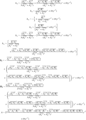
 $$\begin{eqnarray}\displaystyle & \displaystyle u^{\prime +}\underset{y^{+}\rightarrow 0}{{\sim}}A_{u}^{\prime +}(x^{+},z^{+},t^{+})y^{+}+B_{u}^{\prime +}(x^{+},z^{+},t^{+}){y^{+}}^{2}+C_{u}^{\prime +}(x^{+},z^{+},t^{+}){y^{+}}^{3}+\cdots & \displaystyle\end{eqnarray}$$
 $$\begin{eqnarray}\displaystyle & \displaystyle v^{\prime +}\underset{y^{+}\rightarrow 0}{{\sim}}B_{v}^{\prime +}(x^{+},z^{+},t^{+}){y^{+}}^{2}+C_{v}^{\prime +}(x^{+},z^{+},t^{+}){y^{+}}^{3}+\cdots & \displaystyle\end{eqnarray}$$
 $$\begin{eqnarray}\displaystyle & \displaystyle w^{\prime +}\underset{y^{+}\rightarrow 0}{{\sim}}A_{w}^{\prime +}(x^{+},z^{+},t^{+})y^{+}+B_{w}^{\prime +}(x^{+},z^{+},t^{+}){y^{+}}^{2}+C_{w}^{\prime +}(x^{+},z^{+},t^{+}){y^{+}}^{3}+\cdots & \displaystyle\end{eqnarray}$$
 $u_{i}^{\prime }(x,y^{+}=0,z,t)=0$
at the wall (A 2), and the fluctuating continuity equation (3.2a
), whose limit at the wall is
 $\lim _{y^{+}\rightarrow 0}(\unicode[STIX]{x2202}_{y^{+}}v^{\prime +})=0\stackrel{(\text{A}\,1)}{\;\Longrightarrow \;}A_{v}^{\prime +}=0$
, i.e.
 $v^{\prime +}\propto {y^{+}}^{2}$
as
 $y^{+}\rightarrow 0$
(2.3b
). Expansions (2.3) of the near-wall fluctuating velocity field are valid for general three-dimensional (3-D)
 $xyz$
-inhomogeneous turbulent incompressible flow near a plane no-slip wall. Assuming (2.3), straightforward calculations yield the asymptotic expansions of
 $\unicode[STIX]{x1D633}_{ij}^{+}$
and
 $\unicode[STIX]{x1D700}_{ij}^{+}$
, from which (§ A.2) are calculated the asymptotic expansions of
 $\unicode[STIX]{x1D623}_{ij}$
(table 1),
 $\unicode[STIX]{x1D623}_{\unicode[STIX]{x1D700}_{ij}}$
(table 2), and of their invariants (tables 1 and 2). Obviously (tables 1 and 2) the wall values of the anisotropy tensors
 $\unicode[STIX]{x1D623}_{ij}$
and
 $\unicode[STIX]{x1D623}_{\unicode[STIX]{x1D700}_{ij}}$
are identical, and their wall-normal gradients are proportional with factor
 $2$
, viz.
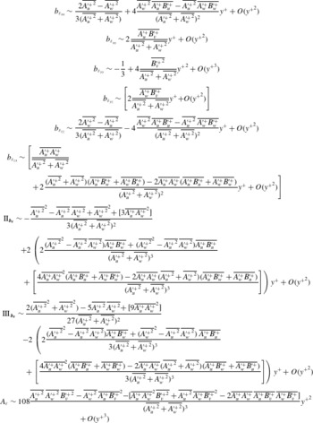
 $$\begin{eqnarray}\displaystyle \unicode[STIX]{x1D623}_{\unicode[STIX]{x1D700}_{ij}}\underset{y^{+}\rightarrow 0}{{\sim}}(\unicode[STIX]{x1D623}_{ij})_{w}+2\left(\frac{\unicode[STIX]{x2202}\unicode[STIX]{x1D623}_{ij}}{\unicode[STIX]{x2202}y^{+}}\right)_{w}y^{+}+O({y^{+}}^{2}), & & \displaystyle\end{eqnarray}$$
with fundamental differences occurring in the
 $O({y^{+}}^{2})$
terms, those of
 $\unicode[STIX]{x1D623}_{\unicode[STIX]{x1D700}_{ij}}$
containing the spatial gradients
 $(\unicode[STIX]{x1D735}A_{u}^{\prime })^{+}$
and
 $(\unicode[STIX]{x1D735}A_{w}^{\prime })^{+}$
, contrary to those of
 $\unicode[STIX]{x1D623}_{ij}$
. Concerning the wall-normal diagonal components,
 $b_{yy}$
and
 $b_{\unicode[STIX]{x1D700}_{yy}}$
, whose linear
 $O(y^{+})$
terms are
 $=0$
, notice that (tables 1 and 2) the wall-normal two-derivatives are proportional with a factor 4
 $$\begin{eqnarray}\displaystyle b_{\unicode[STIX]{x1D700}_{yy}}\underset{y^{+}\rightarrow 0}{{\sim}}(b_{yy})_{w}+4\left(\frac{1}{2}\frac{\unicode[STIX]{x2202}^{2}b_{yy}}{\unicode[STIX]{x2202}{y^{+}}^{2}}\right)_{w}{y^{+}}^{2}+O({y^{+}}^{3}). & & \displaystyle\end{eqnarray}$$
Relation (2.4a ) carries over (tables 1 and 2) to the anisotropy invariants (2.1d–f ) and (2.2d–f )
 $$\begin{eqnarray}\displaystyle & \displaystyle \text{II}_{\boldsymbol{b}_{\unicode[STIX]{x1D73A}}}\underset{y^{+}\rightarrow 0}{{\sim}}(\text{II}_{\boldsymbol{b}})_{w}+2\left(\frac{\unicode[STIX]{x2202}\text{II}_{\boldsymbol{b}}}{\unicode[STIX]{x2202}y^{+}}\right)_{w}y^{+}+O({y^{+}}^{2}) & \displaystyle\end{eqnarray}$$
 $$\begin{eqnarray}\displaystyle & \displaystyle \text{III}_{\boldsymbol{b}_{\unicode[STIX]{x1D73A}}}\underset{y^{+}\rightarrow 0}{{\sim}}(\text{III}_{\boldsymbol{b}})_{w}+2\left(\frac{\unicode[STIX]{x2202}\text{III}_{\boldsymbol{b}}}{\unicode[STIX]{x2202}y^{+}}\right)_{w}y^{+}+O({y^{+}}^{2}). & \displaystyle\end{eqnarray}$$
Consistent with the 2-C componentality of both
 $\unicode[STIX]{x1D633}_{ij}$
(2.1a–c
) and
 $\unicode[STIX]{x1D700}_{ij}$
(2.2a–c
) at the wall (Launder & Shima Reference Launder and Shima1989; Hanjalić Reference Hanjalić1994; Craft & Launder Reference Craft and Launder2001), the wall values of the corresponding Lumley flatness parameters (2.1d–f
) and (2.2d–f
)
 $A_{w}=(A_{\unicode[STIX]{x1D700}})_{w}=0$
(Lumley Reference Lumley1978; Simonsen & Krogstad Reference Simonsen and Krogstad2005). Furthermore, both
 $A$
and
 $A_{\unicode[STIX]{x1D700}}$
tend to
 $0$
quadratically as
 $y^{+}\rightarrow 0$
, and their wall-normal two-derivatives are proportional by a factor 4 (tables 1 and 2)
 $$\begin{eqnarray}\displaystyle & \displaystyle A\underset{y^{+}\rightarrow 0}{{\sim}}O({y^{+}}^{2}) & \displaystyle\end{eqnarray}$$
 $$\begin{eqnarray}\displaystyle & \displaystyle A_{\unicode[STIX]{x1D700}}\underset{y^{+}\rightarrow 0}{{\sim}}4\left(\frac{1}{2}\frac{\unicode[STIX]{x2202}^{2}A}{\unicode[STIX]{x2202}{y^{+}}^{2}}\right)_{w}{y^{+}}^{2}+O({y^{+}}^{3}) & \displaystyle\end{eqnarray}$$
because, as can be verified by straightforward calculation, the constant and linear terms in the expansion of the invariants
 $\{\text{II}_{\boldsymbol{b}},\text{III}_{\boldsymbol{b}},\text{II}_{\boldsymbol{b}_{\unicode[STIX]{x1D73A}}},\text{III}_{\boldsymbol{b}_{\unicode[STIX]{x1D73A}}}\}$
(tables 1 and 2), cancel out
 $$\begin{eqnarray}\displaystyle & \displaystyle 9(\text{II}_{\boldsymbol{b}})_{w}+27(\text{III}_{\boldsymbol{b}})_{w}=9(\text{II}_{\boldsymbol{b}_{\unicode[STIX]{x1D73A}}})_{w}+27(\text{III}_{\boldsymbol{b}_{\unicode[STIX]{x1D73A}}})_{w}=-1 & \displaystyle\end{eqnarray}$$
 $$\begin{eqnarray}\displaystyle & \displaystyle 9\left(\frac{\unicode[STIX]{x2202}\text{II}_{\boldsymbol{b}}}{\unicode[STIX]{x2202}y^{+}}\right)_{w}+27\left(\frac{\unicode[STIX]{x2202}\text{III}_{\boldsymbol{b}}}{\unicode[STIX]{x2202}y^{+}}\right)_{w}=9\left(\frac{\unicode[STIX]{x2202}\text{II}_{\boldsymbol{b}_{\unicode[STIX]{x1D73A}}}}{\unicode[STIX]{x2202}y^{+}}\right)_{w}+27\left(\frac{\unicode[STIX]{x2202}\text{III}_{\boldsymbol{b}_{\unicode[STIX]{x1D73A}}}}{\unicode[STIX]{x2202}y^{+}}\right)_{w}=0. & \displaystyle\end{eqnarray}$$
Of course, calculations retaining the
 $O(y^{+2})$
terms in the expansions of the invariants were required to obtain the result (2.5d
).
Regarding
 $\unicode[STIX]{x1D623}_{ij}$
(table 1), the new results in the paper, with reference to Hanjalić (Reference Hanjalić1994, Tab. 3, p. 191) are the asymptotic expansions of the invariants
 $\text{II}_{\boldsymbol{b}}$
and
 $\text{III}_{\boldsymbol{b}}$
, and in particular of the flatness parameter
 $A$
. Corresponding expansions were obtained (table 2) for
 $\unicode[STIX]{x1D623}_{\unicode[STIX]{x1D700}_{ij}}$
and for its invariants (
 $\text{II}_{\boldsymbol{b}_{\unicode[STIX]{x1D73A}}}$
,
 $\text{III}_{\boldsymbol{b}_{\unicode[STIX]{x1D73A}}}$
,
 $A_{\unicode[STIX]{x1D700}}$
). With regard to the relations between
 $\unicode[STIX]{x1D623}_{ij}$
and
 $\unicode[STIX]{x1D623}_{\unicode[STIX]{x1D700}_{ij}}$
, Mansour et al. (Reference Mansour, Kim and Moin1988, p. 32) have ‘point(ed) out that close to the wall, Taylor series expansions of
 $\unicode[STIX]{x1D623}_{\unicode[STIX]{x1D700}_{ij}}$
and
 $\unicode[STIX]{x1D623}_{ij}$
show that they are equal only up to
 $O(y^{+})$
’; this remark clearly implies
 $(\unicode[STIX]{x1D623}_{\unicode[STIX]{x1D700}_{ij}})_{w}=(\unicode[STIX]{x1D623}_{ij})_{w}$
. The present results (2.4) and (2.5) show the proportionality relation
 $(\unicode[STIX]{x2202}_{y^{+}}\unicode[STIX]{x1D623}_{ij})_{w}\stackrel{(2.4a)}{=}((\unicode[STIX]{x2202}_{y^{+}}\unicode[STIX]{x1D623}_{\unicode[STIX]{x1D700}_{ij}})_{w})/2$
of the wall-normal gradients and the corresponding relation between the wall-normal gradients of the invariants
 $(\unicode[STIX]{x2202}_{y^{+}}\text{II}_{\boldsymbol{b}_{\unicode[STIX]{x1D73A}}})_{w}\stackrel{(2.4c)}{=}2(\unicode[STIX]{x2202}_{y^{+}}\text{II}_{\boldsymbol{b}})_{w}$
and
 $(\unicode[STIX]{x2202}_{y^{+}}\text{III}_{\boldsymbol{b}_{\unicode[STIX]{x1D73A}}})_{w}\stackrel{(2.4d)}{=}2(\unicode[STIX]{x2202}_{y^{+}}\text{III}_{\boldsymbol{b}})_{w}$
on the one hand, and the quadratic asymptotic behaviour of the flatness parameters
 $A_{\unicode[STIX]{x1D700}}\stackrel{(2.5)}{\underset{y^{+}\rightarrow 0}{{\sim}}}4A+O(y^{+3})\stackrel{(2.5a)}{\underset{y^{+}\rightarrow 0}{\propto }}O(y^{+2})$
on the other hand.
2.3
$Re_{\unicode[STIX]{x1D70F}_{w}}$
influence on anisotropy

The evolution of mean flow and turbulence structure with
 $Re_{\unicode[STIX]{x1D70F}_{w}}$
(A 3k
) is central in wall-turbulence research (Marusic et al.
Reference Marusic, Mckeon, Monkewitz, Nagib, Smits and Sreenivasan2010, Reference Marusic, Monty, Hultmark and Smits2013; Kim Reference Kim2012) and DNS of turbulent plane channel flow at progressively higher
 $Re_{\unicode[STIX]{x1D70F}_{w}}$
(Moser et al.
Reference Moser, Kim and Mansour1999; Hoyas & Jiménez Reference Hoyas and Jiménez2006, Reference Hoyas and Jiménez2008; Bernardini et al.
Reference Bernardini, Pirozzoli and Orlandi2014; Lee & Moser Reference Lee and Moser2015) contribute towards answering several open questions on very high
 $Re$
asymptotics. Turbulence structure is generally represented by non-dimensional ratios of turbulent quantities (Bradshaw Reference Bradshaw1967). In this respect, the anisotropy tensors
 $\unicode[STIX]{x1D623}_{ij}$
(2.1a–c
) and
 $\unicode[STIX]{x1D623}_{\unicode[STIX]{x1D700}_{ij}}$
(2.2a–c
), and their AIMs (Lumley & Newman Reference Lumley and Newman1977; Lumley Reference Lumley1978; Lee & Reynolds Reference Lee, Reynolds, Durst, Launder, Lumley, Schmidt and Whitelaw1987; Simonsen & Krogstad Reference Simonsen and Krogstad2005) are particularly useful in understanding the differences in behaviour between the Reynolds stresses
 $\unicode[STIX]{x1D633}_{ij}$
(2.1a–c
) and their dissipation rates
 $\unicode[STIX]{x1D700}_{ij}$
(2.2a–c
), across the channel (in the wall-normal direction
 $y$
) and with varying Reynolds number
 $Re_{\unicode[STIX]{x1D70F}_{w}}$
(A 3k
).
Anisotropy (2.1, 2.2) of the normal (
 $b_{xx}$
,
 $b_{yy}$
,
 $b_{zz}$
) and shear (
 $b_{xy}$
) Reynolds stresses, and of the corresponding dissipation rates (
 $b_{\unicode[STIX]{x1D700}_{xx}}$
,
 $b_{\unicode[STIX]{x1D700}_{yy}}$
,
 $b_{\unicode[STIX]{x1D700}_{zz}}$
,
 $b_{\unicode[STIX]{x1D700}_{xy}}$
), from existing (Moser et al.
Reference Moser, Kim and Mansour1999; del Álamo & Jiménez Reference del Álamo and Jiménez2003; Hoyas & Jiménez Reference Hoyas and Jiménez2006, Reference Hoyas and Jiménez2008; Lee & Moser Reference Lee and Moser2015) DNS computations of turbulent plane channel flow, in the range
 $Re_{\unicode[STIX]{x1D70F}_{w}}\in [180,5200]$
, plotted against the inner-scaled (A 3e–g
) wall distance
 $y^{+}$
(log scale and linear wall zoom).

Near-wall peaks of the streamwise (
 $\max _{y^{+}}b_{xx}$
,
 $\max _{y^{+}}b_{\unicode[STIX]{x1D700}_{xx}}$
) and spanwise (
 $\min _{y^{+}}b_{zz}$
,
 $\min _{y^{+}}b_{\unicode[STIX]{x1D700}_{zz}}$
) components of the anisotropy tensors of the Reynolds stresses
 $\unicode[STIX]{x1D657}$
(2.1) and of the corresponding dissipation rates
 $\unicode[STIX]{x1D657}_{\unicode[STIX]{x1D73A}}$
(2.2), as a function of the friction Reynolds number (A 3k
)
 $Re_{\unicode[STIX]{x1D70F}_{w}}$
(log scale) and of its inverse
 $Re_{\unicode[STIX]{x1D70F}_{w}}^{-1}$
(linear scale), from existing (Moser et al.
Reference Moser, Kim and Mansour1999; Hu et al.
Reference Hu, Morfey and Sandham2006; Hoyas & Jiménez Reference Hoyas and Jiménez2006, Reference Hoyas and Jiménez2008; Lozano-Durán & Jiménez Reference Lozano-Durán and Jiménez2014; Bernardini et al.
Reference Bernardini, Pirozzoli and Orlandi2014; Vreman & Kuerten Reference Vreman and Kuerten2014b
, Reference Vreman and Kuerten2016; Lee & Moser Reference Lee and Moser2015) DNS computations of turbulent plane channel flow in the range
 $Re_{\unicode[STIX]{x1D70F}_{w}}\in [100,5200]$
.

2.3.1 Anisotropy tensors
The strong anisotropy of the Reynolds stresses in wall turbulence is related to the anisotropy of the dissipation-rate tensor
 $\unicode[STIX]{x1D700}_{ij}$
(Gerolymos et al.
Reference Gerolymos, Lo, Vallet and Younis2012b
), and it is established that the behaviour of the anisotropy tensor of the Reynolds stresses
 $\unicode[STIX]{x1D623}_{ij}$
differs from that of the anisotropy tensor of the dissipation rate
 $\unicode[STIX]{x1D623}_{\unicode[STIX]{x1D700}_{ij}}$
(Launder & Reynolds Reference Launder and Reynolds1983; Lai & So Reference Lai and So1990; Jovanović et al.
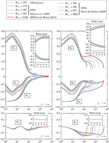
Reference Jovanović, Ye and Durst1995; Jakirlić & Hanjalić Reference Jakirlić and Hanjalić2002). This is obvious by examining (figure 1) existing (Moser et al.
Reference Moser, Kim and Mansour1999; del Álamo & Jiménez Reference del Álamo and Jiménez2003; Hoyas & Jiménez Reference Hoyas and Jiménez2006, Reference Hoyas and Jiménez2008; Lee & Moser Reference Lee and Moser2015) DNS results which include budgets of
 $\unicode[STIX]{x1D633}_{ij}$
transport (and hence data for the components of
 $\unicode[STIX]{x1D700}_{ij}$
) covering the range
 $Re_{\unicode[STIX]{x1D70F}_{w}}\in [178,5186]$
. Recall that (§ 2.2), at the wall (
 $y^{+}=0$
), the anisotropy tensors
 $\unicode[STIX]{x1D623}_{ij}$
and
 $\unicode[STIX]{x1D623}_{\unicode[STIX]{x1D700}_{ij}}$
are identical (Mansour et al.
Reference Mansour, Kim and Moin1988, p. 32), but the wall-normal gradient of
 $\unicode[STIX]{x1D623}_{\unicode[STIX]{x1D700}_{ij}}$
is exactly twice that of
 $\unicode[STIX]{x1D623}_{ij}$
(2.4a
). This explains the near-wall (
 $y^{+}<10$
) evolution of the streamwise (
 $b_{xx}$
,
 $b_{\unicode[STIX]{x1D700}_{xx}}$
) and spanwise (
 $b_{zz}$
,
 $b_{\unicode[STIX]{x1D700}_{zz}}$
) components of the anisotropy tensors (figure 1), viz. that
 $\{b_{\unicode[STIX]{x1D700}_{xx}},|b_{\unicode[STIX]{x1D700}_{zz}}|\}$
increase much faster with
 $y^{+}$
, and reach their maxima at
 $y^{+}\in [3,4]$
, nearer the wall compared to
 $\{b_{xx},|b_{zz}|\}$
which reach their maxima at
 $y^{+}\in [7,9]$
. These near-wall maxima of
 $\{b_{xx},|b_{zz}|,b_{\unicode[STIX]{x1D700}_{xx}},|b_{\unicode[STIX]{x1D700}_{zz}}|\}$
are also global maxima across the channel (figure 1). Notice that at fixed
 $Re_{\unicode[STIX]{x1D70F}_{w}}$
the maximum of the spanwise component occurs at slightly higher
 $y^{+}$
than the maximum of the streamwise component, both for
 $\unicode[STIX]{x1D623}_{ij}$
and
 $\unicode[STIX]{x1D623}_{\unicode[STIX]{x1D700}_{ij}}$
(figure 1). Furthermore, at fixed
 $Re_{\unicode[STIX]{x1D70F}_{w}}$
, the values of the maxima are quite close (
 $\max _{y}b_{xx}\approxeq \max _{y}b_{\unicode[STIX]{x1D700}_{xx}}$
and
 $\max _{y}|b_{zz}|\approxeq \max _{y}|b_{\unicode[STIX]{x1D700}_{zz}}|$
) but
 $\unicode[STIX]{x1D700}_{ij}$
is slightly more anisotropic than
 $\unicode[STIX]{x1D633}_{ij}$
(figure 1). In the near-wall region (
 $y^{+}\lessapprox 10$
), the anisotropy of the streamwise (
 $b_{xx}$
,
 $b_{\unicode[STIX]{x1D700}_{xx}}$
) and spanwise (
 $b_{zz}$
,
 $b_{\unicode[STIX]{x1D700}_{zz}}$
) components decreases with increasing
 $Re_{\unicode[STIX]{x1D70F}_{w}}$
, first quite sharply (
 $Re_{\unicode[STIX]{x1D70F}_{w}}<400$
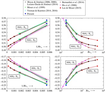
) and then more slowly (figure 1). Careful examination of the values of the maxima versus
 $Re_{\unicode[STIX]{x1D70F}_{w}}$
(figure 2) suggests that they probably tend to
 $Re_{\unicode[STIX]{x1D70F}_{w}}$
-independent values as
 $Re_{\unicode[STIX]{x1D70F}_{w}}$
increases, although these are not reached yet at the highest available
 $Re_{\unicode[STIX]{x1D70F}_{w}}\approxeq 5186$
DNS of Lee & Moser (Reference Lee and Moser2015). To alleviate the bias of the computational grid, the values of the extrema were determined by fitting a degree-four interpolating polynomial
 $p_{I}(y^{+})$
around the on-grid extremum (two neighbours on each side) and solving
 $p_{I}^{\prime }(y^{+})=0$
by Newton iteration. This generally had no influence on the value of the maximum, but did smooth out variations of its location. Plots (figure 2) of the near-wall peaks of the streamwise (
 $\max _{y^{+}}b_{xx}$
,
 $\max _{y^{+}}b_{\unicode[STIX]{x1D700}_{xx}}$
) and spanwise (
 $\min _{y^{+}}b_{zz}$
,
 $\min _{y^{+}}b_{\unicode[STIX]{x1D700}_{zz}}$
) components versus
 $Re_{\unicode[STIX]{x1D70F}_{w}}$
(log scale) hint that asymptotic limits are approached, and this is further verified by plotting the data against
 $Re_{\unicode[STIX]{x1D70F}_{w}}^{-1}$
(figure 2). More sets of data are available for
 $\unicode[STIX]{x1D633}_{ij}$
than for
 $\unicode[STIX]{x1D700}_{ij}$
, and two slightly distinct curves appear for the
 $\unicode[STIX]{x1D623}_{ij}$
-extrema (figure 2), but this only affects the precise value of the asymptotic limits as
 $Re_{\unicode[STIX]{x1D70F}_{w}}^{-1}\rightarrow 0$
(
 ${\sim}2\,\%$
scatter for
 $\max _{y^{+}}b_{xx}$
and
 ${\sim}5\,\%$
scatter for
 $\min _{y^{+}}b_{zz}$
). The anisotropy of the wall-normal component is of course highest at the 2-C wall
 $(b_{yy})_{w}=(b_{\unicode[STIX]{x1D700}_{yy}})_{w}=-1/3$
and then becomes less anisotropic with increasing
 $y^{+}$
(figure 1). Obviously, the coefficient
 $\unicode[STIX]{x1D700}_{w}^{+-1}\overline{B_{v}^{\prime +2}}$
(tables 1 and 2) of the leading quadratic term in (2.4b
) slightly increases with increasing
 $Re_{\unicode[STIX]{x1D70F}_{w}}$
(figure 1). Finally, regarding the shear components, both
 $b_{xy}$
and
 $b_{\unicode[STIX]{x1D700}_{xy}}$
seem
 $Re_{\unicode[STIX]{x1D70F}_{w}}$
independent near the wall (
 $y^{+}\lessapprox 10$
).
In contrast to the near-wall region (
 $y^{+}\lessapprox 10$
), which is dominated by the wall-asymptotic relations (§ 2.2), the behaviour of
 $\unicode[STIX]{x1D623}_{\unicode[STIX]{x1D700}_{ij}}$
is completely different from that of
 $\unicode[STIX]{x1D623}_{ij}$
at higher
 $y^{+}$
(figure 1). The anisotropy of the streamwise Reynolds-stress component
 $b_{xx}$
forms, with increasing
 $Re_{\unicode[STIX]{x1D70F}_{w}}$
, a plateau corresponding to the log region of the mean velocity profile (Coles Reference Coles1956) followed by a sharp decrease in the wake region. The level of anisotropy
 $b_{xx}$
in the log region increases with
 $Re_{\unicode[STIX]{x1D70F}_{w}}$
but may be reaching an asymptotic limit, although simulations at higher
 $Re_{\unicode[STIX]{x1D70F}_{w}}$
are needed to ascertain this point. The spanwise component
 $b_{zz}$
becomes more isotropic with increasing
 $y^{+}$
in the buffer layer (
 $y^{+}\in [10,100]$
), followed by a slight increase in anisotropy in the log region (figure 1), while the wall-normal component
 $b_{yy}$
becomes more isotropic with increasing
 $y^{+}$
, quite sharply in the buffer layer and more progressively in the log region. Interestingly, both
 $b_{yy}$
and
 $b_{zz}$
also seem to be forming a log-region plateau with increasing
 $Re_{\unicode[STIX]{x1D70F}_{w}}$
, but simulations at higher
 $Re_{\unicode[STIX]{x1D70F}_{w}}$
are required to verify this trend. Both components
 $b_{yy}$
and
 $b_{zz}$
become more anisotropic in the log region with increasing
 $Re_{\unicode[STIX]{x1D70F}_{w}}$
(figure 1). Finally, in the wake region, both
 $b_{yy}$
and
 $b_{zz}$
tend quite sharply to a common centreline value (figure 1).
Contrary to
 $\unicode[STIX]{x1D623}_{ij}$
, the diagonal components of
 $\unicode[STIX]{x1D623}_{\unicode[STIX]{x1D700}_{ij}}$
tend quasi-monotonically to a near-isotropic (but not exactly isotropic) state at the centreline, first steeply in the buffer layer and then more gradually in the log region (figure 1). The low-
 $Re_{\unicode[STIX]{x1D70F}_{w}}$
data exhibit a clear albeit slight increase in the anisotropy of
 $\{b_{\unicode[STIX]{x1D700}_{xx}},b_{\unicode[STIX]{x1D700}_{yy}},b_{\unicode[STIX]{x1D700}_{zz}}\}$
near the centreline which becomes less pronounced with increasing
 $Re_{\unicode[STIX]{x1D70F}_{w}}$
. Unlike
 $b_{zz}$
,
 $b_{\unicode[STIX]{x1D700}_{zz}}$
reaches a near-zero value in the log region (figure 1).
The shear components also behave very differently. The Reynolds-stress anisotropy
 $b_{xy}$
becomes more anisotropic from the wall up to the beginning of the wake region, before sharply going to zero (exactly, because of the symmetry condition
 $\overline{u^{\prime }v^{\prime }}|_{CL}=0$
) at the centreline. The shear component
 $b_{\unicode[STIX]{x1D700}_{xy}}$
is practically
 $Re_{\unicode[STIX]{x1D70F}_{w}}$
independent up to the end of the buffer layer (
 $y^{+}\lessapprox 100$
), with a wavy shape reaching zero near
 $y^{+}\approxeq 20$
(figure 1), then being relatively flat in the log region.
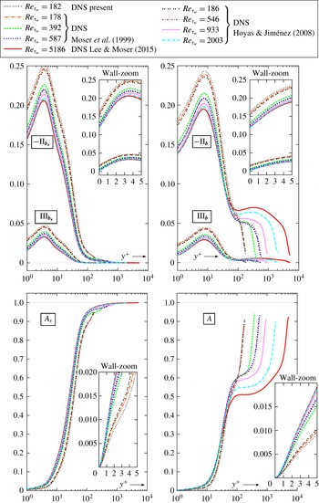
Invariants of the anisotropy tensors (2.1, 2.2) of the Reynolds stresses
 $\unicode[STIX]{x1D657}$
(
 $\text{II}_{\boldsymbol{b}}$
,
 $\text{III}_{\boldsymbol{b}}$
) and of the corresponding dissipation rates
 $\unicode[STIX]{x1D657}_{\unicode[STIX]{x1D73A}}$
(
 $\text{II}_{\boldsymbol{b}_{\unicode[STIX]{x1D73A}}}$
,
 $\text{III}_{\boldsymbol{b}_{\unicode[STIX]{x1D73A}}}$
), and Lumley’s (Reference Lumley1978) flatness parameters (
 $A:=1+27\text{III}_{\boldsymbol{b}}+\text{II}_{\boldsymbol{b}}$
and
 $A_{\unicode[STIX]{x1D700}}:=1+27\text{III}_{\boldsymbol{b}_{\unicode[STIX]{x1D73A}}}+\text{II}_{\boldsymbol{b}_{\unicode[STIX]{x1D73A}}}$
), from existing (Moser et al.
Reference Moser, Kim and Mansour1999; del Álamo & Jiménez Reference del Álamo and Jiménez2003; Hoyas & Jiménez Reference Hoyas and Jiménez2006, Reference Hoyas and Jiménez2008; Lee & Moser Reference Lee and Moser2015) DNS computations of turbulent plane channel flow, in the range
 $Re_{\unicode[STIX]{x1D70F}_{w}}\in [180,5200]$
, plotted against the inner-scaled (A 3e–g
) wall distance
 $y^{+}$
(log scale and linear wall zoom).

2.3.2 Anisotropy invariants
More precise information on the influence of
 $Re_{\unicode[STIX]{x1D70F}_{w}}$
(A 3k
) on the anisotropy of
 $\unicode[STIX]{x1D633}_{ij}$
and
 $\unicode[STIX]{x1D700}_{ij}$
can be obtained by considering the invariants
 $\{\text{III}_{\boldsymbol{b}},-\text{II}_{\boldsymbol{b}}\}$
(2.1d–f
) and
 $\{\text{III}_{\boldsymbol{b}_{\unicode[STIX]{x1D73A}}},-\text{II}_{\boldsymbol{b}_{\unicode[STIX]{x1D73A}}}\}$
(2.2d–f
) whose locus lies inside Lumley’s (Reference Lumley1978) realizability triangle (Mansour et al.
Reference Mansour, Kim and Moin1988, figures 17 and 18, p. 32). As the intervals of possible values (Lumley Reference Lumley1978; Simonsen & Krogstad Reference Simonsen and Krogstad2005)
 $$\begin{eqnarray}\displaystyle & \displaystyle \text{II}_{\boldsymbol{b}}\in [-{\textstyle \frac{1}{3}},0]\ni \text{II}_{\boldsymbol{b}_{\unicode[STIX]{x1D73A}}} & \displaystyle\end{eqnarray}$$
 $$\begin{eqnarray}\displaystyle & \displaystyle \text{III}_{\boldsymbol{b}}\in [-{\textstyle \frac{1}{108}},{\textstyle \frac{2}{27}}]\ni \text{III}_{\boldsymbol{b}_{\unicode[STIX]{x1D73A}}} & \displaystyle\end{eqnarray}$$
 $$\begin{eqnarray}\displaystyle & \displaystyle A\in [0,1]\ni A_{\unicode[STIX]{x1D700}} & \displaystyle\end{eqnarray}$$
 $Re_{\unicode[STIX]{x1D70F}_{w}}$
on the near-wall peaks of the invariants (figure 3). The evolution of the invariants with
 $y^{+}$
and
 $Re_{\unicode[STIX]{x1D70F}_{w}}$
(figure 3) is very similar to what was observed for the diagonal components of the anisotropy tensors (figure 1). Near the wall,
 $\{\text{III}_{\boldsymbol{b}_{\unicode[STIX]{x1D73A}}},-\text{II}_{\boldsymbol{b}_{\unicode[STIX]{x1D73A}}}\}$
increase faster with
 $y^{+}$
compared to
 $\{\text{III}_{\boldsymbol{b}},-\text{II}_{\boldsymbol{b}}\}$
, in line with (2.4c
) and (2.4d
), reaching their maxima at
 $y^{+}\in [3,4]$
compared to
 $y^{+}\in [7,9]$
(figure 3),
 $\unicode[STIX]{x1D700}_{ij}$
being slightly more anisotropic than
 $\unicode[STIX]{x1D633}_{ij}$
. Near the wall,
 $A_{\unicode[STIX]{x1D700}}$
increases much faster with
 $y^{+}$
compared to
 $A$
(figure 3), in line with (2.5a
) and (2.5b
). There is noticeable
 $Re_{\unicode[STIX]{x1D70F}_{w}}$
-influence for
 $Re_{\unicode[STIX]{x1D70F}_{w}}<400$
both in wall values and in rate of increase with
 $y^{+}$
for all of the invariants (figure 3). On the other hand, with increasing
 $Re_{\unicode[STIX]{x1D70F}_{w}}$
, it would seem that an asymptotic state is approached in the near-wall region, including the buffer layer (
 $y^{+}\lessapprox 100$
), although DNS at higher
 $Re_{\unicode[STIX]{x1D70F}_{w}}$
are still required to fully substantiate this observation. Regarding the invariants of
 $\unicode[STIX]{x1D633}_{ij}$
,
 $\{-\text{II}_{\boldsymbol{b}},\text{III}_{\boldsymbol{b}},A\}$
, a plateau appears with increasing
 $Re_{\unicode[STIX]{x1D70F}_{w}}$
(figure 3), marking the log region of the mean velocity profile (Lee & Moser Reference Lee and Moser2015), but again DNS at higher
 $Re_{\unicode[STIX]{x1D70F}_{w}}$
are needed to determine whether a
 $Re_{\unicode[STIX]{x1D70F}_{w}}$
-asymptotic value of the level of this plateau exists. On the contrary, the invariants of
 $\unicode[STIX]{x1D700}_{ij}$
 $\{-\text{II}_{\boldsymbol{b}_{\unicode[STIX]{x1D73A}}},\text{III}_{\boldsymbol{b}_{\unicode[STIX]{x1D73A}}},A_{\unicode[STIX]{x1D700}}\}$
vary monotonically from the wall to centreline, and seem to approach
 $Re_{\unicode[STIX]{x1D70F}_{w}}$
-independent
 $y^{+}$
-distributions with increasing
 $Re_{\unicode[STIX]{x1D70F}_{w}}$
.
2.3.3 AIM at the wall and at the centreline
The variation with
 $Re_{\unicode[STIX]{x1D70F}_{w}}$
of the
 $y^{+}$
-distributions of
 $\unicode[STIX]{x1D633}_{ij}$
and
 $\unicode[STIX]{x1D700}_{ij}$
anisotropy (figures 1–3) indicates trends in the evolution of turbulence structure with increasing
 $Re_{\unicode[STIX]{x1D70F}_{w}}$
. These trends are better quantified by studying the evolution with
 $Re_{\unicode[STIX]{x1D70F}_{w}}$
of the anisotropy invariants (
 $-\text{II}_{\boldsymbol{b}}$
,
 $\text{III}_{\boldsymbol{b}}$
,
 $-\text{II}_{\boldsymbol{b}_{\unicode[STIX]{x1D73A}}}$
,
 $\text{III}_{\boldsymbol{b}_{\unicode[STIX]{x1D73A}}}$
) at the wall and at the centreline (figure 4). Several of the available DNS data (Kim et al.
Reference Kim, Moin and Moser1987; Moser et al.
Reference Moser, Kim and Mansour1999; Hu et al.
Reference Hu, Morfey and Sandham2002, Reference Hu, Morfey and Sandham2003, Reference Hu, Morfey and Sandham2006; del Álamo & Jiménez Reference del Álamo and Jiménez2003; Hoyas & Jiménez Reference Hoyas and Jiménez2006, Reference Hoyas and Jiménez2008; Lozano-Durán & Jiménez Reference Lozano-Durán and Jiménez2014; Bernardini et al.
Reference Bernardini, Pirozzoli and Orlandi2014; Vreman & Kuerten Reference Vreman and Kuerten2014a
,Reference Vreman and Kuerten
b
, Reference Vreman and Kuerten2016; Lee & Moser Reference Lee and Moser2015) acquired since the pioneering work of Kim et al. (Reference Kim, Moin and Moser1987) were considered in this study. These data were obtained by several authors with different computational accuracy indicators (spatio-temporal resolution, box size, observation time and sampling frequency) using a variety of computational methods and/or codes. Notice that for the low
 $Re_{\unicode[STIX]{x1D70F}_{w}}\approxeq 180$
case, Vreman & Kuerten (Reference Vreman and Kuerten2014a
) recently reported a detailed study demonstrating consistent convergence of DNS results with increasing computational accuracy. At the centreline, only databases including
 $\unicode[STIX]{x1D700}_{ij}$
-data (Moser et al.
Reference Moser, Kim and Mansour1999; del Álamo & Jiménez Reference del Álamo and Jiménez2003; Hoyas & Jiménez Reference Hoyas and Jiménez2006, Reference Hoyas and Jiménez2008; Vreman & Kuerten Reference Vreman and Kuerten2014b
, Reference Vreman and Kuerten2016), were used for the
 $\unicode[STIX]{x1D657}_{\unicode[STIX]{x1D73A}}$
-invariants (figure 4), and wall values for the
 $\unicode[STIX]{x1D657}_{\unicode[STIX]{x1D73A}}$
invariants were used when available (Moser et al.
Reference Moser, Kim and Mansour1999; del Álamo & Jiménez Reference del Álamo and Jiménez2003; Hoyas & Jiménez Reference Hoyas and Jiménez2006, Reference Hoyas and Jiménez2008). For those databases that did not include wall values (Vreman & Kuerten Reference Vreman and Kuerten2014b
, Reference Vreman and Kuerten2016) or
 $\unicode[STIX]{x1D700}_{ij}$
-data (Hu et al.
Reference Hu, Morfey and Sandham2006; Bernardini et al.
Reference Bernardini, Pirozzoli and Orlandi2014; Lozano-Durán & Jiménez Reference Lozano-Durán and Jiménez2014) wall invariants were estimated by linear extrapolation of the
 $\unicode[STIX]{x1D657}$
invariants from the first 2 grid points. The very-near-wall (
 $y^{+}\lessapprox 0.2$
) data of Bernardini et al. (Reference Bernardini, Pirozzoli and Orlandi2014) were noisy (presumably because of the extreme near-wall cosine stretching of the wall-normal mesh size) and were not used; corresponding wall values were obtained by extrapolation from the first 2 grid points with
 $y^{+}\gtrapprox 0.2$
. The
 $Re_{\unicode[STIX]{x1D70F}_{w}}\approxeq 4180$
small-box data of Lozano-Durán & Jiménez (Reference Lozano-Durán and Jiménez2014) were only used at the wall. Finally, it was found interesting to include the
 $Re_{\unicode[STIX]{x1D70F}_{w}}<180$
data of Hu et al. (Reference Hu, Morfey and Sandham2002, Reference Hu, Morfey and Sandham2003, Reference Hu, Morfey and Sandham2006) illustrating low-
 $Re_{\unicode[STIX]{x1D70F}_{w}}$
asymptotics.
It should be stated from the outset that anisotropy invariants are much more sensitive to
 $\unicode[STIX]{x1D633}_{ij}$
and
 $\unicode[STIX]{x1D700}_{ij}$
data uncertainties (Schultz & Flack Reference Schultz and Flack2013, p. 5) because of the cumulative propagation of these uncertainties (Taylor Reference Taylor1997, § 3, pp. 45–91) in the calculation of the anisotropy tensors (2.1a–c
) and (2.2a–c
), and then of their invariants (2.1a–c
) and (2.2a–c
). Nonetheless, although data for some of the invariants exhibit substantial scatter (figure 4), it appears that
 $Re_{\unicode[STIX]{x1D70F}_{w}}$
-trends can be deduced with reasonable confidence.
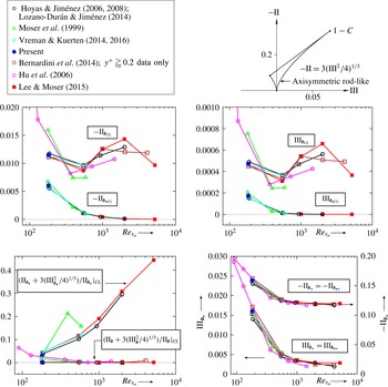
Invariants of the anisotropy tensors (2.1, 2.2) of the Reynolds-stresses
 $\unicode[STIX]{x1D657}$
(
 $\text{II}_{\boldsymbol{b}}$
,
 $\text{III}_{\boldsymbol{b}}$
) and of the corresponding dissipation rates
 $\unicode[STIX]{x1D657}_{\unicode[STIX]{x1D73A}}$
(
 $\text{II}_{\boldsymbol{b}_{\unicode[STIX]{x1D73A}}}$
,
 $\text{III}_{\boldsymbol{b}_{\unicode[STIX]{x1D73A}}}$
), at the wall
 $(\cdot )_{w}$
and at channel centreline
 $(\cdot )_{CL}$
, and axisymmetry diagnostic
 $\text{II}_{\boldsymbol{b}}^{-1}(\text{II}_{\boldsymbol{b}}+3(\text{III}_{\boldsymbol{b}}^{2}/4)^{1/3})$
and
 $\text{II}_{\boldsymbol{b}_{\unicode[STIX]{x1D73A}}}^{-1}(\text{II}_{\boldsymbol{b}_{\unicode[STIX]{x1D73A}}}+3(\text{III}_{\boldsymbol{b}_{\unicode[STIX]{x1D73A}}}^{2}/4)^{1/3})$
, at the centreline
 $(\cdot )_{CL}$
, as a function of the friction Reynolds number
 $Re_{\unicode[STIX]{x1D70F}_{w}}$
(A 3k
), from existing (Moser et al.
Reference Moser, Kim and Mansour1999; Hu et al.
Reference Hu, Morfey and Sandham2006; Hoyas & Jiménez Reference Hoyas and Jiménez2006, Reference Hoyas and Jiménez2008; Bernardini et al.
Reference Bernardini, Pirozzoli and Orlandi2014; Lozano-Durán & Jiménez Reference Lozano-Durán and Jiménez2014; Vreman & Kuerten Reference Vreman and Kuerten2014b
, Reference Vreman and Kuerten2016; Lee & Moser Reference Lee and Moser2015) DNS computations of turbulent plane channel flow, in the range
 $Re_{\unicode[STIX]{x1D70F}_{w}}\in [80,5200]$
.

At the wall, the data for both
 ${\text{II}_{\boldsymbol{b}}}_{w}\stackrel{(2.4c)}{=}{\text{II}_{\boldsymbol{b}_{\unicode[STIX]{x1D73A}}}}_{w}$
and
 ${\text{III}_{\boldsymbol{b}}}_{w}\stackrel{(2.4d)}{=}{\text{III}_{\boldsymbol{b}_{\unicode[STIX]{x1D73A}}}}_{w}$
show consistent behaviour with reasonably small scatter (figure 4) suggesting that the near-wall DNS data are quite robust with respect to the variation of computational accuracy indicators of the simulations. It seems likely that, with increasing
 $Re_{\unicode[STIX]{x1D70F}_{w}}$
, the wall invariants reach asymptotic values. On the other hand, as
 $Re_{\unicode[STIX]{x1D70F}_{w}}$
decreases, both invariants increase sharply (figure 4). Notice that the very-small-box
 $Re_{\unicode[STIX]{x1D70F}_{w}}\approxeq 4180$
data of Lozano-Durán & Jiménez (Reference Lozano-Durán and Jiménez2014), which were only considered at the wall, are consistent with the large-box data (Bernardini et al.
Reference Bernardini, Pirozzoli and Orlandi2014; Lee & Moser Reference Lee and Moser2015) suggesting that the small-box bias mainly impacts the centreline region, whereas the very-near-wall behaviour is less sensitive to the details of the large-scale outer-flow structures.
At the centreline, the data show considerable scatter (figure 4), especially for the
 $\unicode[STIX]{x1D657}$
invariants
 $(-\text{II}_{\boldsymbol{b}},\text{III}_{\boldsymbol{b}})_{CL}$
, in line with the observation on the cumulative impact of
 $\unicode[STIX]{x1D633}_{ij}$
and
 $\unicode[STIX]{x1D700}_{ij}$
uncertainties on the calculation of the invariants. Notice first that the scatter is more important for the
 $\unicode[STIX]{x1D657}$
invariants which characterize (Lee & Reynolds Reference Lee, Reynolds, Durst, Launder, Lumley, Schmidt and Whitelaw1987) the large-scale anisotropy and are therefore more sensitive to box size and observation time, whereas the
 $\unicode[STIX]{x1D657}_{\unicode[STIX]{x1D73A}}$
invariants
 $(-\text{II}_{\boldsymbol{b}_{\unicode[STIX]{x1D73A}}},\text{III}_{\boldsymbol{b}_{\unicode[STIX]{x1D73A}}})_{CL}$
which characterize the small-scale anisotropy are more robust. With respect to box size, notice that high
 $Re_{\unicode[STIX]{x1D70F}_{w}}$
small-box calculations (Lozano-Durán & Jiménez Reference Lozano-Durán and Jiménez2014) overpredict the
 $\unicode[STIX]{x1D657}$
-invariants at the centreline by a factor 2 (not included in figure 4). This is not completely unexpected, and, in view of the consistent wall invariants obtained in these high-
 $Re_{\unicode[STIX]{x1D70F}_{w}}$
small-box calculations, it suggests that the very-large-scale structures influence quite substantially turbulence at the centreline and much less in the very-near-wall (sublayer) region. The general trend of the
 $\unicode[STIX]{x1D657}$
invariants
 $(-\text{II}_{\boldsymbol{b}},\text{III}_{\boldsymbol{b}})_{CL}$
at the centreline (figure 4), is a strong decrease with increasing
 $Re_{\unicode[STIX]{x1D70F}_{w}}$
in the range
 $Re_{\unicode[STIX]{x1D70F}_{w}}<400$
, followed by a slight increase, probably reaching an asymptotic state with increasing
 $Re_{\unicode[STIX]{x1D70F}_{w}}$
. Nonetheless there is too much scatter in the data to draw definitive conclusions (figure 4). Regarding the
 $\unicode[STIX]{x1D657}_{\unicode[STIX]{x1D73A}}$
invariants
 $(-\text{II}_{\boldsymbol{b}_{\unicode[STIX]{x1D73A}}},\text{III}_{\boldsymbol{b}_{\unicode[STIX]{x1D73A}}})_{CL}$
at the centreline, there appears a clear trend of asymptotic decrease to
 $\approxeq 0$
as
 $Re_{\unicode[STIX]{x1D70F}_{w}}$
increases (figure 4).
Observation of
 $\unicode[STIX]{x1D623}_{ij}$
at the centreline (figure 1), where by symmetry
 $b_{xy_{CL}}=0$
, shows that
 $b_{yy_{CL}}\approxeq b_{zz_{CL}}<b_{xx_{CL}}$
(figure 1), at least for
 $Re_{\unicode[STIX]{x1D70F}_{w}}\geqslant 180$
, implying that the Reynolds-stress tensor at the centreline is axisymmetric rod-like (Simonsen & Krogstad Reference Simonsen and Krogstad2005, figure 4, p. 3). However, the componentality of
 $\unicode[STIX]{x1D700}_{ij}$
at the centreline is not as obvious (figure 1), especially as the
 $\unicode[STIX]{x1D657}_{\unicode[STIX]{x1D73A}}$
invariants approach zero at the centreline (figure 4), contrary to the
 $\unicode[STIX]{x1D657}$
invariants which seem to reach finite asymptotic values at the centreline (figure 4). At the rod-like axisymmetric boundary of the realizability triangle (figure 4)
 $\text{II}+3(\text{III}^{2}/4)^{1/3}=0$
, so that
 $\text{II}^{-1}(\text{II}+3(\text{III}^{2}/4)^{1/3})$
is a diagnostic function whose distance from zero denotes departure from rod-like axisymmetric componentality. Contrary to
 $\unicode[STIX]{x1D657}_{CL}$
,
 $\unicode[STIX]{x1D657}_{\unicode[STIX]{x1D73A}CL}$
at the centreline seems to become increasingly non-axisymmetric as
 $Re_{\unicode[STIX]{x1D70F}_{w}}$
increases (figure 4). Finally, the data of Hu et al. (Reference Hu, Morfey and Sandham2006) at very low
 $Re_{\unicode[STIX]{x1D70F}_{w}}<180$
seem to indicate departure from rod-like axisymmetry for
 $\unicode[STIX]{x1D657}_{CL}$
(figure 4). At
 $Re_{\unicode[STIX]{x1D70F}_{w}}\approxeq 180$
, the data of Kim et al. (Reference Kim, Moin and Moser1987) also indicate a slight departure from rod-like axisymmetry of
 $\unicode[STIX]{x1D657}_{CL}$
, but all other data (Hoyas & Jiménez Reference Hoyas and Jiménez2006; Bernardini et al.
Reference Bernardini, Pirozzoli and Orlandi2014; Lee & Moser Reference Lee and Moser2015; Vreman & Kuerten Reference Vreman and Kuerten2016), including the present calculations, indicate that
 $\unicode[STIX]{x1D657}_{CL}$
is rod-like axisymmetric at
 $Re_{\unicode[STIX]{x1D70F}_{w}}\approxeq 180$
(figure 4). Further DNS at very low
 $Re_{\unicode[STIX]{x1D70F}_{w}}<180$
are therefore needed to verify the departure from rod-like axisymmetry of
 $\unicode[STIX]{x1D657}_{CL}$
with decreasing
 $Re_{\unicode[STIX]{x1D70F}_{w}}$
.
3
$\unicode[STIX]{x1D700}_{ij}$
-budgets

The dynamics of
 $\unicode[STIX]{x1D700}_{ij}$
is described by an exact transport equation that can be readily obtained by the fluctuating flow equations (§ 3.1). The budgets of the various terms in the transport equations for
 $\unicode[STIX]{x1D700}_{ij}$
(3.3) are studied for low Reynolds number plane channel flow (§ 3.2).
Notice first that
 $\unicode[STIX]{x1D700}_{ij}$
(1.2a
) is generated from the four-order tensor
 $$\begin{eqnarray}\displaystyle {\mathcal{E}}_{ijkm}:=2\unicode[STIX]{x1D708}\overline{\frac{\unicode[STIX]{x2202}u_{i}^{\prime }}{\unicode[STIX]{x2202}x_{k}}\frac{\unicode[STIX]{x2202}u_{j}^{\prime }}{\unicode[STIX]{x2202}x_{m}}}\stackrel{(1.2a)}{\;\Longrightarrow \;}\unicode[STIX]{x1D700}_{ij}={\mathcal{E}}_{ijkm}\unicode[STIX]{x1D6FF}_{km}={\mathcal{E}}_{ijkk} & & \displaystyle\end{eqnarray}$$
by contraction of the last two indices. Considering
 ${\mathcal{E}}_{ijkm}$
is important because this four-order tensor appears in the production mechanisms of
 $\unicode[STIX]{x1D700}_{ij}$
(3.3). The tensor
 ${\mathcal{E}}_{ijkm}$
was used by other authors (Durbin & Speziale Reference Durbin and Speziale1991; Speziale & Gatski Reference Speziale and Gatski1997) who studied
 $\unicode[STIX]{x1D700}_{ij}$
transport in homogeneous turbulence. It is also interesting to note that the nine transport equations for the variances of the fluctuating velocity gradients studied by Vreman & Kuerten (Reference Vreman and Kuerten2014b
, (7, 9), p. 4) are also included in the transport equations for
 ${\mathcal{E}}_{ijkm}$
(3.1a
) because
 $$\begin{eqnarray}\displaystyle 2\unicode[STIX]{x1D708}\overline{\left(\frac{\unicode[STIX]{x2202}u_{i}^{\prime }}{\unicode[STIX]{x2202}x_{j}}\right)^{2}}\in \{{\mathcal{E}}_{xxxx},{\mathcal{E}}_{xxyy},{\mathcal{E}}_{xxzz},{\mathcal{E}}_{yyxx},{\mathcal{E}}_{yyyy},{\mathcal{E}}_{yyzz},{\mathcal{E}}_{zzxx},{\mathcal{E}}_{zzyy},{\mathcal{E}}_{zzzz}\}. & & \displaystyle\end{eqnarray}$$
3.1
$\unicode[STIX]{x1D700}_{ij}$
-transport equation

Starting from the fluctuating continuity (Mathieu & Scott Reference Mathieu and Scott2000, (4.6), p. 76)
 $$\begin{eqnarray}\displaystyle \frac{\unicode[STIX]{x2202}u_{\ell }^{\prime }}{\unicode[STIX]{x2202}x_{\ell }}=0 & & \displaystyle\end{eqnarray}$$
and fluctuating momentum (Mathieu & Scott Reference Mathieu and Scott2000, (4.31), p. 85)
 $$\begin{eqnarray}\displaystyle \unicode[STIX]{x1D70C}\frac{\unicode[STIX]{x2202}u_{i}^{\prime }}{\unicode[STIX]{x2202}t}+\unicode[STIX]{x1D70C}\bar{u}_{\ell }\frac{\unicode[STIX]{x2202}u_{i}^{\prime }}{\unicode[STIX]{x2202}x_{\ell }}=-\unicode[STIX]{x1D70C}\frac{\unicode[STIX]{x2202}}{\unicode[STIX]{x2202}x_{\ell }}(u_{i}^{\prime }u_{\ell }^{\prime }-\overline{u_{i}^{\prime }u_{\ell }^{\prime }})-\unicode[STIX]{x1D70C}u_{\ell }^{\prime }\frac{\unicode[STIX]{x2202}\bar{u}_{i}}{\unicode[STIX]{x2202}x_{\ell }}-\frac{\unicode[STIX]{x2202}p^{\prime }}{\unicode[STIX]{x2202}x_{i}}+\unicode[STIX]{x1D707}\frac{\unicode[STIX]{x2202}^{2}u_{i}^{\prime }}{\unicode[STIX]{x2202}x_{\ell }\unicode[STIX]{x2202}x_{\ell }} & & \displaystyle\end{eqnarray}$$
equations we can work out the transport equations for
 ${\mathcal{E}}_{ijkm}$
(3.1a
), and by contraction (3.1a
) the transport equation for
 $\unicode[STIX]{x1D700}_{ij}$
, which reads
 $$\begin{eqnarray}\displaystyle & & \displaystyle \underbrace{\unicode[STIX]{x1D70C}\frac{\unicode[STIX]{x2202}\unicode[STIX]{x1D700}_{ij}}{\unicode[STIX]{x2202}t}+\unicode[STIX]{x1D70C}\bar{u}_{\ell }\frac{\unicode[STIX]{x2202}\unicode[STIX]{x1D700}_{ij}}{\unicode[STIX]{x2202}x_{\ell }}}_{C_{\unicode[STIX]{x1D700}_{ij}}}=\underbrace{\frac{\unicode[STIX]{x2202}}{\unicode[STIX]{x2202}x_{\ell }}\left[\unicode[STIX]{x1D707}\frac{\unicode[STIX]{x2202}\unicode[STIX]{x1D700}_{ij}}{\unicode[STIX]{x2202}x_{\ell }}\right]}_{d_{\unicode[STIX]{x1D700}_{ij}}^{(\unicode[STIX]{x1D707})}}+\underbrace{\frac{\unicode[STIX]{x2202}}{\unicode[STIX]{x2202}x_{\ell }}\left[-\unicode[STIX]{x1D70C}\left(\overline{u_{\ell }^{\prime }2\unicode[STIX]{x1D708}\frac{\unicode[STIX]{x2202}u_{i}^{\prime }}{\unicode[STIX]{x2202}x_{k}}\frac{\unicode[STIX]{x2202}u_{j}^{\prime }}{\unicode[STIX]{x2202}x_{k}}}\right)\right]}_{d_{\unicode[STIX]{x1D700}_{ij}}^{(u)}}\nonumber\\ \displaystyle & & \displaystyle \quad \underbrace{-\unicode[STIX]{x1D70C}\unicode[STIX]{x1D700}_{i\ell }\frac{\unicode[STIX]{x2202}\bar{u}_{j}}{\unicode[STIX]{x2202}x_{\ell }}-\unicode[STIX]{x1D70C}\unicode[STIX]{x1D700}_{j\ell }\frac{\unicode[STIX]{x2202}\bar{u}_{i}}{\unicode[STIX]{x2202}x_{\ell }}}_{P_{\unicode[STIX]{x1D700}_{ij}}^{(1)}}\underbrace{-\unicode[STIX]{x1D70C}\left(2\unicode[STIX]{x1D708}\overline{\frac{\unicode[STIX]{x2202}u_{i}^{\prime }}{\unicode[STIX]{x2202}x_{k}}\frac{\unicode[STIX]{x2202}u_{j}^{\prime }}{\unicode[STIX]{x2202}x_{\ell }}}\right)\left(\frac{\unicode[STIX]{x2202}\bar{u}_{k}}{\unicode[STIX]{x2202}x_{\ell }}+\frac{\unicode[STIX]{x2202}\bar{u}_{\ell }}{\unicode[STIX]{x2202}x_{k}}\right)}_{P_{\unicode[STIX]{x1D700}_{ij}}^{(2)}}\nonumber\\ \displaystyle & & \displaystyle \quad \underbrace{-\unicode[STIX]{x1D70C}\!\left(2\unicode[STIX]{x1D708}\overline{u_{\ell }^{\prime }\frac{\unicode[STIX]{x2202}u_{i}^{\prime }}{\unicode[STIX]{x2202}x_{k}}}\right)\frac{\unicode[STIX]{x2202}^{2}\bar{u}_{j}}{\unicode[STIX]{x2202}x_{\ell }\unicode[STIX]{x2202}x_{k}}-\unicode[STIX]{x1D70C}\!\left(2\unicode[STIX]{x1D708}\overline{u_{\ell }^{\prime }\frac{\unicode[STIX]{x2202}u_{j}^{\prime }}{\unicode[STIX]{x2202}x_{k}}}\right)\frac{\unicode[STIX]{x2202}^{2}\bar{u}_{i}}{\unicode[STIX]{x2202}x_{\ell }\unicode[STIX]{x2202}x_{k}}}_{P_{\unicode[STIX]{x1D700}_{ij}}^{(3)}}\underbrace{-\unicode[STIX]{x1D70C}\!\left[\!2\unicode[STIX]{x1D708}\overline{\frac{\unicode[STIX]{x2202}u_{\ell }^{\prime }}{\unicode[STIX]{x2202}x_{k}}\left(\frac{\unicode[STIX]{x2202}u_{i}^{\prime }}{\unicode[STIX]{x2202}x_{k}}\frac{\unicode[STIX]{x2202}u_{j}^{\prime }}{\unicode[STIX]{x2202}x_{\ell }}+\frac{\unicode[STIX]{x2202}u_{j}^{\prime }}{\unicode[STIX]{x2202}x_{k}}\frac{\unicode[STIX]{x2202}u_{i}^{\prime }}{\unicode[STIX]{x2202}x_{\ell }}\right)}\right]}_{\unicode[STIX]{x1D6EF}_{\unicode[STIX]{x1D700}_{ij}}=:P_{\unicode[STIX]{x1D700}_{ij}}^{(4)}}\nonumber\\ \displaystyle & & \displaystyle \quad \underbrace{-2\unicode[STIX]{x1D708}\overline{\frac{\unicode[STIX]{x2202}u_{i}^{\prime }}{\unicode[STIX]{x2202}x_{k}}\frac{\unicode[STIX]{x2202}^{2}p^{\prime }}{\unicode[STIX]{x2202}x_{j}\unicode[STIX]{x2202}x_{k}}}-2\unicode[STIX]{x1D708}\overline{\frac{\unicode[STIX]{x2202}u_{j}^{\prime }}{\unicode[STIX]{x2202}x_{k}}\frac{\unicode[STIX]{x2202}^{2}p^{\prime }}{\unicode[STIX]{x2202}x_{i}\unicode[STIX]{x2202}x_{k}}}}_{\unicode[STIX]{x1D6F1}_{\unicode[STIX]{x1D700}_{ij}}}-\underbrace{\unicode[STIX]{x1D70C}\overline{\left(2\unicode[STIX]{x1D708}\frac{\unicode[STIX]{x2202}^{2}u_{i}^{\prime }}{\unicode[STIX]{x2202}x_{k}\unicode[STIX]{x2202}x_{\ell }}\right)\left(2\unicode[STIX]{x1D708}\frac{\unicode[STIX]{x2202}^{2}u_{j}^{\prime }}{\unicode[STIX]{x2202}x_{k}\unicode[STIX]{x2202}x_{\ell }}\right)}}_{\unicode[STIX]{x1D70C}\unicode[STIX]{x1D700}_{\unicode[STIX]{x1D700}_{ij}}}.\end{eqnarray}$$
In (3.3)
 $C_{\unicode[STIX]{x1D700}_{ij}}$
is the convection of
 $\unicode[STIX]{x1D700}_{ij}$
by the mean-flow velocity field
 $\bar{u}_{\ell }$
,
 $d_{\unicode[STIX]{x1D700}_{ij}}^{(\unicode[STIX]{x1D707})}$
is the diffusion of
 $\unicode[STIX]{x1D700}_{ij}$
by molecular viscosity (notice that
 $d_{\unicode[STIX]{x1D700}_{ij}}^{(\unicode[STIX]{x1D707})}\stackrel{(3.3)}{=}\unicode[STIX]{x1D707}\unicode[STIX]{x1D6FB}^{2}\unicode[STIX]{x1D700}_{ij}$
for
 $\unicode[STIX]{x1D707}=\text{const.}$
),
 $d_{\unicode[STIX]{x1D700}_{ij}}^{(u)}$
is the turbulent diffusion (mixing) of
 $\unicode[STIX]{x1D700}_{ij}$
by the fluctuating velocity field
 $u_{\ell }^{\prime }$
,
 $P_{\unicode[STIX]{x1D700}_{ij}}^{(1)}$
is the production of
 $\unicode[STIX]{x1D700}_{ij}$
by the action of its components on the mean-flow velocity gradients,
 $P_{\unicode[STIX]{x1D700}_{ij}}^{(2)}$
is the production of
 $\unicode[STIX]{x1D700}_{ij}$
by the action of
 ${\mathcal{E}}_{ijkm}$
(3.1) on the mean-flow velocity gradients,
 $P_{\unicode[STIX]{x1D700}_{ij}}^{(3)}$
is the production of
 $\unicode[STIX]{x1D700}_{ij}$
by the mean-flow velocity Hessian,
 $P_{\unicode[STIX]{x1D700}_{ij}}^{(4)}:=\unicode[STIX]{x1D6EF}_{\unicode[STIX]{x1D700}_{ij}}$
corresponds to triple correlations of fluctuating velocity gradients whose trace
 $(\unicode[STIX]{x1D6EF}_{\unicode[STIX]{x1D700}_{\ell \ell }})/2$
was identified by Mansour et al. (Reference Mansour, Kim and Moin1988) as a term ‘producing’ (gain in the budgets of)
 $\unicode[STIX]{x1D700}:=\unicode[STIX]{x1D700}_{\ell \ell }/2$
(by extension the denomination
 $P_{\unicode[STIX]{x1D700}_{ij}}^{(4)}$
is used, although this term does not contain gradients of the mean-flow field),
 $\unicode[STIX]{x1D6F1}_{\unicode[STIX]{x1D700}_{ij}}$
are the terms containing the fluctuating pressure Hessian, and
 $\unicode[STIX]{x1D700}_{\unicode[STIX]{x1D700}_{ij}}$
is the destruction of
 $\unicode[STIX]{x1D700}_{ij}$
by the action of molecular viscosity. Following usual practice (Mansour et al.
Reference Mansour, Kim and Moin1988, (1), p. 17) for the incompressible
 $\unicode[STIX]{x1D633}_{ij}$
equations (1.1) and for the
 $\unicode[STIX]{x1D700}$
equation (Mansour et al.
Reference Mansour, Kim and Moin1988, (23), p. 23), a computable viscous diffusion term
 $d_{\unicode[STIX]{x1D700}_{ij}}^{(\unicode[STIX]{x1D707})}$
was chosen in (3.3), with a corresponding appropriate definition of the destruction-of-dissipation tensor
 $\unicode[STIX]{x1D700}_{\unicode[STIX]{x1D700}_{ij}}$
(3.3), in lieu of alternative splittings based on the viscous-stress tensor (Ben Nasr, Gerolymos & Vallet Reference Ben Nasr, Gerolymos and Vallet2014, (2), p. 189).
Using (3.1) the production of
 $\unicode[STIX]{x1D700}_{ij}$
by mean-flow velocity gradients reads
 $$\begin{eqnarray}\displaystyle P_{\unicode[STIX]{x1D700}_{ij}}^{(1)}+P_{\unicode[STIX]{x1D700}_{ij}}^{(2)}\stackrel{(3.3,3.1a)}{=}\underbrace{-\unicode[STIX]{x1D70C}{\mathcal{E}}_{i\ell kk}\frac{\unicode[STIX]{x2202}\bar{u}_{j}}{\unicode[STIX]{x2202}x_{\ell }}-\unicode[STIX]{x1D70C}{\mathcal{E}}_{j\ell kk}\frac{\unicode[STIX]{x2202}\bar{u}_{i}}{\unicode[STIX]{x2202}x_{\ell }}}_{P_{\unicode[STIX]{x1D700}_{ij}}^{(1)}}\underbrace{-\unicode[STIX]{x1D70C}{\mathcal{E}}_{ijk\ell }\left(\frac{\unicode[STIX]{x2202}\bar{u}_{k}}{\unicode[STIX]{x2202}x_{\ell }}+\frac{\unicode[STIX]{x2202}\bar{u}_{\ell }}{\unicode[STIX]{x2202}x_{k}}\right)}_{P_{\unicode[STIX]{x1D700}_{ij}}^{(2)}} & & \displaystyle\end{eqnarray}$$
highlighting the importance of considering the generating fourth-order tensor
 ${\mathcal{E}}_{ijkm}$
(3.1). The separation in two terms,
 $P_{\unicode[STIX]{x1D700}_{ij}}^{(1)}$
and
 $P_{\unicode[STIX]{x1D700}_{ij}}^{(2)}$
, was made to distinguish between the computable (from the knowledge of
 $\unicode[STIX]{x1D700}_{ij}$
and the mean-flow field) term
 $P_{\unicode[STIX]{x1D700}_{ij}}^{(1)}$
, and
 $P_{\unicode[STIX]{x1D700}_{ij}}^{(2)}$
which involves components of
 ${\mathcal{E}}_{ijkm}$
that do not simplify by contraction (3.1a
) to
 $\unicode[STIX]{x1D700}_{ij}$
.
3.2
$\unicode[STIX]{x1D700}_{ij}$
-transport budgets

Budgets of the
 $\unicode[STIX]{x1D700}_{ij}$
-transport equations (3.3), for turbulent plane channel flow, were obtained (figure 5) in an
 $L_{x}\times L_{y}\times L_{z}=4\unicode[STIX]{x03C0}\unicode[STIX]{x1D6FF}\times 2\unicode[STIX]{x1D6FF}\times 4/3\unicode[STIX]{x03C0}\unicode[STIX]{x1D6FF}$
computational box, using a carefully validated DNS solver (Gerolymos et al.
Reference Gerolymos, Sénéchal and Vallet2010, Reference Gerolymos, Sénéchal and Vallet2013; Gerolymos & Vallet Reference Gerolymos and Vallet2014). The resolution in the homogeneous
 $xz$
-directions is
 $\unicode[STIX]{x0394}x^{+}\approxeq 5.7$
and
 $\unicode[STIX]{x0394}z^{+}\approxeq 1.9$
. The wall-normal size of the grid cells adjacent to the wall was
 $\unicode[STIX]{x0394}y_{w}^{+}\approxeq 0.22$
. More importantly, the mesh (65 % of the nodes were stretched near the walls geometrically with ratio
 $r_{j}=1.0427$
, the remaining nodes in the outer region being equidistant) was kept fine in the entire near-wall region, with
 $N_{y^{+}\leqslant 10}=26$
grid cells between the wall and
 $y^{+}\approxeq 10$
, and remained fine up to the centreline where the wall-normal cell size was
 $\unicode[STIX]{x0394}y_{CL}^{+}\approxeq 3.1$
. This spatial resolution, combined with the
 $O(\unicode[STIX]{x0394}\ell ^{17})$
scheme used (Gerolymos et al.
Reference Gerolymos, Sénéchal and Vallet2009, Reference Gerolymos, Sénéchal and Vallet2010) is quite fine in view of current state-of-the-art DNS at this
 $Re_{\unicode[STIX]{x1D70F}_{w}}\approxeq 180$
(Vreman & Kuerten Reference Vreman and Kuerten2014a
, Reference Vreman and Kuerten2016). Statistics was acquired at high sampling frequency (at every iteration;
 $\unicode[STIX]{x0394}t_{s}^{+}=\unicode[STIX]{x0394}t^{+}\approxeq 0.0060$
, albeit for a relatively short observation time
 $t_{OBS}^{+}\approxeq 777$
). The close agreement (§ 4) of the present results for the budgets of the diagonal components with the highly resolved computations of Vreman & Kuerten (Reference Vreman and Kuerten2016) further substantiate the validity of the computations. Wall asymptotics of the various terms in (3.3) can be obtained using the Taylor expansions (2.3) in the fluctuating momentum equations (3.2b
). Although a full report of these calculations is outside the scope of this paper, some of the limiting wall values obtained from this procedure are included in the following discussion.
Regarding the streamwise component
 $\unicode[STIX]{x1D700}_{xx}^{+}$
(figure 5), production
 $P_{\unicode[STIX]{x1D700}_{xx}}^{+}$
(gain) roughly balances destruction
 $-\unicode[STIX]{x1D700}_{\unicode[STIX]{x1D700}_{xx}}^{+}$
(loss) in the major part of the channel (
 $y^{+}\gtrapprox 1$
), with lesser contributions of diffusion (
 $d_{\unicode[STIX]{x1D700}_{xx}}^{(u)+}+d_{\unicode[STIX]{x1D700}_{xx}}^{(\unicode[STIX]{x1D707})+}$
). Production
 $P_{\unicode[STIX]{x1D700}_{xx}}^{+}$
peaks at
 $y^{+}\approxeq 4$
and destruction
 $\unicode[STIX]{x1D700}_{\unicode[STIX]{x1D700}_{xx}}^{+}$
at
 $y^{+}\approxeq 5$
. The pressure term
 $\unicode[STIX]{x1D6F1}_{\unicode[STIX]{x1D700}_{xx}}^{+}$
is negligible in the budgets of
 $\unicode[STIX]{x1D700}_{xx}^{+}$
throughout the channel. Very near the wall (
 $y^{+}\lessapprox 1$
; figure 5) production
 $P_{\unicode[STIX]{x1D700}_{xx}}^{+}\underset{y^{+}\rightarrow 0}{\rightarrow 0}$
(wall-asymptotic expansion; § 2.2) and viscous diffusion
 $d_{\unicode[STIX]{x1D700}_{xx}}^{(\unicode[STIX]{x1D707})+}$
(gain
 $\forall y^{+}\lessapprox 1$
) roughly counters destruction
 $-\unicode[STIX]{x1D700}_{\unicode[STIX]{x1D700}_{xx}}^{+}$
(
 $y^{+}\rightarrow 0$
; figure 5). At the wall, the pressure term
 $[\unicode[STIX]{x1D6F1}_{\unicode[STIX]{x1D700}_{xx}}^{+}]_{w}=8\overline{B_{v}^{\prime }\unicode[STIX]{x2202}_{x}A_{u}^{\prime }}^{+}\neq 0$
(wall-asymptotic expansion; § 2.2). However
 $|\unicode[STIX]{x1D6F1}_{\unicode[STIX]{x1D700}_{xx}}^{+}|_{w}\ll [\unicode[STIX]{x1D700}_{\unicode[STIX]{x1D700}_{xx}}^{+}]_{w}\approxeq [d_{\unicode[STIX]{x1D700}_{xx}}^{(\unicode[STIX]{x1D707})+}]_{w}$
(figure 5).
Budgets, in wall units (A 3j
), of the transport equations (3.3) for the dissipation tensor
 $\unicode[STIX]{x1D700}_{ij}$
(1.2a
), from the present DNS computations of turbulent plane channel flow (
 $Re_{\unicode[STIX]{x1D70F}_{w}}\approxeq 182$
,
 $\bar{M}_{CL}\approxeq 0.35$
), plotted against the inner-scaled (A 3e–g
) wall distance
 $y^{+}$
(log scale and linear wall zoom).

The budgets of the spanwise component
 $\unicode[STIX]{x1D700}_{zz}^{+}$
(figure 5) are also dominated by a balance between production
 $P_{\unicode[STIX]{x1D700}_{zz}}^{+}$
(gain) and destruction
 $-\unicode[STIX]{x1D700}_{\unicode[STIX]{x1D700}_{zz}}^{+}$
(loss) in the major part of the channel (
 $y^{+}\gtrapprox 5$
). However, production
 $P_{\unicode[STIX]{x1D700}_{zz}}^{+}$
peaks at
 $y^{+}\approxeq 10$
and becomes negligible at
 $y^{+}\approxeq 3$
as
 $P_{\unicode[STIX]{x1D700}_{zz}}^{+}\underset{y^{+}\rightarrow 0}{\rightarrow 0}$
(wall-asymptotic expansion; § 2.2). In the near-wall region, again destruction
 $-\unicode[STIX]{x1D700}_{\unicode[STIX]{x1D700}_{zz}}^{+}$
(loss
 $\forall y^{+}$
) is balanced by viscous diffusion
 $d_{\unicode[STIX]{x1D700}_{zz}}^{(\unicode[STIX]{x1D707})+}$
(gain
 $\forall y^{+}\lessapprox 6$
), but this zone extends further away from the wall (
 $y^{+}\lessapprox 3$
; figure 5) compared to the streamwise component (
 $y^{+}\lessapprox 1$
; figure 5). As for the streamwise component, the other mechanisms,
 $d_{\unicode[STIX]{x1D700}_{zz}}^{(u)+}$
and
 $\unicode[STIX]{x1D6F1}_{\unicode[STIX]{x1D700}_{zz}}^{+}$
, have a very small contribution to the
 $\unicode[STIX]{x1D700}_{zz}^{+}$
-budget. Another difference between the streamwise and the spanwise components is that
 $\unicode[STIX]{x1D700}_{\unicode[STIX]{x1D700}_{zz}}^{+}$
is maximum at the wall decreasing monotonically with
 $y^{+}$
, contrary to
 $\unicode[STIX]{x1D700}_{\unicode[STIX]{x1D700}_{xx}}^{+}$
(figure 5).
The major difference in the budgets of the wall-normal component
 $\unicode[STIX]{x1D700}_{yy}^{+}$
, compared to the other two diagonal components, is the importance of the pressure term
 $\unicode[STIX]{x1D6F1}_{\unicode[STIX]{x1D700}_{yy}}^{+}$
which is the dominant gain mechanism throughout the channel (figure 5), except very near the wall (
 $y^{+}\lessapprox 1/2$
; figure 5) where
 $\unicode[STIX]{x1D6F1}_{\unicode[STIX]{x1D700}_{yy}}^{+}\underset{y^{+}\rightarrow 0}{\rightarrow 0}$
(wall-asymptotic expansion; § 2.2) and, as for
 $\unicode[STIX]{x1D700}_{xx}^{+}$
and
 $\unicode[STIX]{x1D700}_{zz}^{+}$
, viscous diffusion
 $d_{\unicode[STIX]{x1D700}_{yy}}^{(\unicode[STIX]{x1D707})+}$
(gain) balances destruction
 $-\unicode[STIX]{x1D700}_{\unicode[STIX]{x1D700}_{yy}}^{+}$
(
 $y^{+}\lessapprox 1/2$
; figure 5). Production
 $P_{\unicode[STIX]{x1D700}_{yy}}^{+}$
(gain) is significant in the buffer region (
 $10\lessapprox y^{+}\lessapprox 100$
; figure 5) although it becomes comparable to
 $\unicode[STIX]{x1D6F1}_{\unicode[STIX]{x1D700}_{yy}}^{+}$
only for
 $y^{+}\gtrapprox 100$
(figure 5). Turbulent diffusion
 $d_{\unicode[STIX]{x1D700}_{yy}}^{(u)+}$
is generally weak throughout the channel (figure 5).
The budgets of the shear component
 $\unicode[STIX]{x1D700}_{xy}^{+}<0\,\forall y^{+}>0$
(Mansour et al.
Reference Mansour, Kim and Moin1988, figure 4, p. 19) exhibit a fundamentally different behaviour compared to the diagonal components (figure 5). All of the terms in the
 $\unicode[STIX]{x1D700}_{xy}^{+}$
-budgets (
 $P_{\unicode[STIX]{x1D700}_{xy}}^{+}$
,
 $\unicode[STIX]{x1D6F1}_{\unicode[STIX]{x1D700}_{xy}}^{+}$
,
 $d_{\unicode[STIX]{x1D700}_{xy}}^{(u)+}$
,
 $d_{\unicode[STIX]{x1D700}_{xy}}^{(\unicode[STIX]{x1D707})+}$
,
 $-\unicode[STIX]{x1D700}_{\unicode[STIX]{x1D700}_{xy}}^{+}$
) are significant (figure 5). Contrary to the diagonal components, the destruction term
 $-\unicode[STIX]{x1D700}_{\unicode[STIX]{x1D700}_{xy}}^{+}$
contributes as gain to the budgets in the major part of the channel (
 $y^{+}\gtrapprox 3$
; figure 5), becoming an actual destruction mechanism (loss) only in the viscous sublayer (
 $y^{+}\lessapprox 3$
; figure 5). Notice that, at the wall, viscous diffusion of the shear component is substantially weaker than the two other mechanisms present in (3.3), viz.
 $|\unicode[STIX]{x1D6F1}_{\unicode[STIX]{x1D700}_{xy}}^{+}|_{w}\gg |d_{\unicode[STIX]{x1D700}_{xy}}^{(\unicode[STIX]{x1D707})+}|_{w}=|\unicode[STIX]{x1D700}_{\unicode[STIX]{x1D700}_{xy}}^{+}-\unicode[STIX]{x1D6F1}_{\unicode[STIX]{x1D700}_{xy}}^{+}|_{w}\ll |\unicode[STIX]{x1D700}_{\unicode[STIX]{x1D700}_{xy}}^{+}|_{w}$
(wall-asymptotic expansion; § 2.2; figure 5). In a large part of the channel,
 $-\unicode[STIX]{x1D700}_{\unicode[STIX]{x1D700}_{xy}}^{+}<0\,\forall y^{+}\gtrapprox 3$
(figure 5) is an important gain mechanism, along with production
 $P_{\unicode[STIX]{x1D700}_{xy}}^{+}<0\,\forall y^{+}>0$
(figure 5). On the other hand,
 $\unicode[STIX]{x1D6F1}_{\unicode[STIX]{x1D700}_{xy}}^{+}$
is the main loss mechanism in the major part of the channel (figure 5). Notice the complicated
 $y^{+}$
-evolution of
 $\unicode[STIX]{x1D6F1}_{\unicode[STIX]{x1D700}_{xy}}^{+}$
(figure 5), which is
 ${<}0$
(gain) at the wall, crossing to
 ${>}0$
(loss) at
 $y^{+}\gtrapprox 1/2$
, and presents a plateau (
 $3\lessapprox y^{+}\lessapprox 7$
) followed by a global maximum at
 $y^{+}\approxeq 15$
, before decreasing monotonically to
 $0$
at the centreline. In the region
 $1\lessapprox y^{+}\lessapprox 20$
, both diffusion mechanisms,
 $d_{\unicode[STIX]{x1D700}_{xy}}^{(\unicode[STIX]{x1D707})+}$
and
 $d_{\unicode[STIX]{x1D700}_{xy}}^{(u)+}$
, contribute significantly to the
 $\unicode[STIX]{x1D700}_{xy}$
-budgets (figure 5).
A major difference between the
 $\unicode[STIX]{x1D633}_{ij}$
-budgets (Mansour et al.
Reference Mansour, Kim and Moin1988) and the
 $\unicode[STIX]{x1D700}_{ij}$
-budgets (figure 5) lies in the production mechanisms
 $P_{ij}$
(1.1) and
 $P_{\unicode[STIX]{x1D700}_{ij}}$
(3.3). In the
 $\unicode[STIX]{x1D633}_{ij}$
-budgets of plane channel flow, only
 $P_{xx}^{+}\neq 0\neq P_{xy}^{+}$
whereas
 $P_{yy}^{+}=P_{zz}^{+}=0\,\forall y^{+}$
(Mansour et al.
Reference Mansour, Kim and Moin1988, figures 2 and 3, pp. 18–19). On the contrary, all of the components
 $P_{\unicode[STIX]{x1D700}_{ij}}\neq 0\,\forall y^{+}>0$
in general (figure 5). In relation to the above observation, the main gain mechanism in the
 $\unicode[STIX]{x1D700}_{zz}^{+}$
-budgets is production
 $P_{\unicode[STIX]{x1D700}_{zz}}^{+}$
(figure 5) in contrast to the
 $r_{zz}$
-budgets (Mansour et al.
Reference Mansour, Kim and Moin1988, figure 3, p. 19) where, in the absence of production
 $P_{zz}^{+}=0\,\forall y^{+}$
, the pressure term
 $\unicode[STIX]{x1D6F1}_{zz}^{+}$
is the main gain mechanism. On the contrary,
 $\unicode[STIX]{x1D6F1}_{\unicode[STIX]{x1D700}_{zz}}^{+}$
has negligible contribution to the
 $\unicode[STIX]{x1D700}_{zz}$
-budgets (figure 5). It is noteworthy that the importance of the pressure terms
 $\unicode[STIX]{x1D6F1}_{\unicode[STIX]{x1D700}_{yy}}^{+}$
and
 $\unicode[STIX]{x1D6F1}_{\unicode[STIX]{x1D700}_{xy}}^{+}$
in the budgets of the
 $\unicode[STIX]{x1D700}_{yy}^{+}$
and
 $\unicode[STIX]{x1D700}_{xy}^{+}$
components (figure 5) are also quite generally observed in the budgets of wall-normal fluxes, including the Reynolds stresses
 $r_{yy}^{+}$
(Mansour et al.
Reference Mansour, Kim and Moin1988, figure 2, p. 18) and
 $r_{xy}^{+}$
(Mansour et al.
Reference Mansour, Kim and Moin1988, figure 4, p. 19), and in the compressible case, the fluxes of thermodynamic quantities such as temperature
 $\overline{T^{\prime }v^{\prime }}$
(Gerolymos & Vallet Reference Gerolymos and Vallet2014, figures 14 and 15, pp. 737–738), density
 $\overline{\unicode[STIX]{x1D70C}^{\prime }v^{\prime }}$
(Gerolymos & Vallet Reference Gerolymos and Vallet2014, figure 12, p. 731), pressure
 $\overline{p^{\prime }v^{\prime }}$
(Gerolymos & Vallet Reference Gerolymos and Vallet2014, figure 16, p. 741) and entropy
 $\overline{s^{\prime }v^{\prime }}$
(Gerolymos & Vallet Reference Gerolymos and Vallet2014, figure 13, p. 734).
Comparison of the various mechanisms of production
 $P_{\unicode[STIX]{x1D700}_{ij}}=P_{\unicode[STIX]{x1D700}_{ij}}^{(1)}+P_{\unicode[STIX]{x1D700}_{ij}}^{(2)}+P_{\unicode[STIX]{x1D700}_{ij}}^{(3)}+P_{\unicode[STIX]{x1D700}_{ij}}^{(4)}$
(3.3) of the dissipation tensor
 $\unicode[STIX]{x1D700}_{ij}$
(1.2a
), in wall units (A 3j
), from the present DNS computations of turbulent plane channel flow (
 $Re_{\unicode[STIX]{x1D70F}_{w}}\approxeq 182$
,
 $\bar{M}_{CL}\approxeq 0.35$
), plotted against the inner-scaled (A 3e–g
) wall distance
 $y^{+}$
(log scale and linear wall zoom).

Components of different mechanisms of production
 $P_{\unicode[STIX]{x1D700}_{ij}}=P_{\unicode[STIX]{x1D700}_{ij}}^{(1)}+P_{\unicode[STIX]{x1D700}_{ij}}^{(2)}+P_{\unicode[STIX]{x1D700}_{ij}}^{(3)}+P_{\unicode[STIX]{x1D700}_{ij}}^{(4)}$
(3.3) for fully developed turbulent plane channel.

Production
 $P_{\unicode[STIX]{x1D700}_{ij}}^{+}$
(figure 5) of
 $\unicode[STIX]{x1D700}_{ij}$
contains four different mechanisms,
 $P_{\unicode[STIX]{x1D700}_{ij}}^{+}=P_{\unicode[STIX]{x1D700}_{ij}}^{(1)+}+P_{\unicode[STIX]{x1D700}_{ij}}^{(2)+}+P_{\unicode[STIX]{x1D700}_{ij}}^{(3)+}+P_{\unicode[STIX]{x1D700}_{ij}}^{(4)+}$
(3.3), which behave differently for each component across the channel (figure 6). Globally, in plane channel flow,
 $P_{\unicode[STIX]{x1D700}_{ij}}^{+}$
contributes as a gain mechanism in the
 $\unicode[STIX]{x1D700}_{ij}$
-budgets (figures 5 and 6), except very near the wall for the wall-normal (
 $P_{\unicode[STIX]{x1D700}_{yy}}^{+}\leqslant 0\,\forall y^{+}\lessapprox 3$
is a loss mechanism; figure 5) and spanwise (
 $P_{\unicode[STIX]{x1D700}_{zz}}^{+}\leqslant 0\,\forall y^{+}\lessapprox 2$
is a loss mechanism; figure 5) diagonal components. For both the spanwise and wall-normal components,
 $P_{\unicode[STIX]{x1D700}_{yy}}^{(1)+}=P_{\unicode[STIX]{x1D700}_{zz}}^{(1)+}=P_{\unicode[STIX]{x1D700}_{yy}}^{(3)+}=P_{\unicode[STIX]{x1D700}_{zz}}^{(3)+}=0\,\forall y^{+}$
(table 3), whereas production by the action of
 ${\mathcal{E}}_{ijkm}^{+}$
-components on the mean velocity gradient,
 $P_{\unicode[STIX]{x1D700}_{yy}}^{(2)+}$
and
 $P_{\unicode[STIX]{x1D700}_{zz}}^{(2)+}$
(table 3), is the main gain mechanism in the initial part of the buffer layer (
 $y^{+}\in [5,30]$
; figure 6) and is replaced further away from the wall (
 $y^{+}\gtrapprox 30$
; figure 6) by production by triple correlations of fluctuating velocity gradients,
 $P_{\unicode[STIX]{x1D700}_{yy}}^{(4)+}$
and
 $P_{\unicode[STIX]{x1D700}_{zz}}^{(4)+}$
(3.3), as expected from the quasi-homogeneous analysis of Tennekes & Lumley (Reference Tennekes and Lumley1972, pp. 88–92). All of the four production mechanisms (3.3) are active for the streamwise
 $\unicode[STIX]{x1D700}_{xx}^{+}$
and shear
 $\unicode[STIX]{x1D700}_{xy}^{+}$
components (figure 6). Regarding the streamwise component
 $\unicode[STIX]{x1D700}_{xx}^{+}$
, the three mechanisms,
 $P_{\unicode[STIX]{x1D700}_{xx}}^{(1)+}>0$
,
 $P_{\unicode[STIX]{x1D700}_{xx}}^{(2)+}>0$
and
 $P_{\unicode[STIX]{x1D700}_{xx}}^{(4)+}>0\,\forall y^{+}>0$
(figure 6) always contribute as gain to the budgets. On the other hand, production by the mean velocity Hessian,
 $P_{\unicode[STIX]{x1D700}_{xx}}^{(3)+}<0\,\forall y^{+}\lessapprox 10$
(loss) near the wall (figure 6), switching to
 $P_{\unicode[STIX]{x1D700}_{xx}}^{(3)+}>0\,\forall y^{+}\gtrapprox 10$
(gain) further away from the wall, is generally weaker than the other three mechanisms. Notice that the production by the triple correlations of the fluctuating velocity gradients
 $P_{\unicode[STIX]{x1D700}_{xx}}^{(4)+}$
(3.3) is important throughout the channel, even as
 $y^{+}\rightarrow 0$
(figure 6), becoming the dominant mechanism in the outer part of the flow (
 $y^{+}\gtrapprox 15$
; figure 6). Regarding the shear component
 $\unicode[STIX]{x1D700}_{xy}^{+}$
,
 $P_{\unicode[STIX]{x1D700}_{xy}}^{(1)+}=-\unicode[STIX]{x1D700}_{yy}^{+}[d_{y}\bar{u}]^{+}<0\,\forall y^{+}>0$
(figure 6) is the main gain mechanism throughout the channel, whereas
 $P_{\unicode[STIX]{x1D700}_{xy}}^{(2)+}>0$
and
 $P_{\unicode[STIX]{x1D700}_{xy}}^{(3)+}>0\,\forall y^{+}>0$
contribute as loss to the budgets (figure 6). Finally,
 $P_{\unicode[STIX]{x1D700}_{xy}}^{(4)+}<0\,\forall y^{+}\lessapprox 6$
(gain) near the wall (figure 6) switches to
 $P_{\unicode[STIX]{x1D700}_{xy}}^{(4)+}>0\,\forall y^{+}\gtrapprox 6$
(loss) further away from the wall. Interestingly,
 $P_{\unicode[STIX]{x1D700}_{xy}}^{(4)+}$
, although comparable to the other three mechanisms
 $\forall y^{+}$
(figure 6), never becomes the dominant mechanism, even as
 $y^{+}\rightarrow \unicode[STIX]{x1D6FF}^{+}$
, raising the question of applicability of the quasi-homogeneous order-of-magnitude analysis (Tennekes & Lumley Reference Tennekes and Lumley1972, pp. 88–92) to the shear component (although higher-
 $Re$
data are required to fully resolve this issue).
In plane channel flow, production by interaction with the mean velocity gradient
 $P_{\unicode[STIX]{x1D700}_{ij}}^{(1)+}+P_{\unicode[STIX]{x1D700}_{ij}}^{(2)+}$
(3.3) involves
 $\unicode[STIX]{x1D700}_{xy}^{+}$
in
 $P_{\unicode[STIX]{x1D700}_{xx}}^{(1)+}$
(table 3),
 $\unicode[STIX]{x1D700}_{yy}^{+}$
in
 $P_{\unicode[STIX]{x1D700}_{xy}}^{(1)+}$
(table 3), and five different components of
 ${\mathcal{E}}_{ijkm}$
(3.1) in
 $P_{\unicode[STIX]{x1D700}_{ij}}^{(2)+}$
(table 3), which are not involved in the generating relation (3.1a
). Since the mean velocity gradient
 $d_{y}\bar{u}^{+}>0\,\forall y^{+}\in ]0,\unicode[STIX]{x1D6FF}^{+} [$
(Coles Reference Coles1956), the sign of these components directly determines (table 3) whether the corresponding contribution to
 $P_{\unicode[STIX]{x1D700}_{ij}}^{+}$
is gain or loss (figures 6 and 7).
Concerning
 $P_{\unicode[STIX]{x1D700}_{xx}}^{(1)+}$
and
 $P_{\unicode[STIX]{x1D700}_{xx}}^{(2)+}$
(table 3), the corresponding producing components,
 $\unicode[STIX]{x1D700}_{xy}^{+}$
and
 ${\mathcal{E}}_{xxxy}^{+}$
are of comparable magnitude (figure 7), but
 $\unicode[STIX]{x1D700}_{xy}^{+}$
is active nearer to the wall (peak at
 $y^{+}\in [4,5]$
; figure 7) compared to
 ${\mathcal{E}}_{xxxy}^{+}$
(peak at
 $y^{+}\approxeq 15$
; figure 7). Therefore,
 $P_{\unicode[STIX]{x1D700}_{xx}}^{(1)+}$
peaks at
 $y^{+}\in [4,5]$
whereas
 $P_{\unicode[STIX]{x1D700}_{xx}}^{(2)+}$
peaks at
 $y^{+}\approxeq 9$
(figure 6). Near the wall (wall-asymptotic expansion; § 2.2),
 $P_{\unicode[STIX]{x1D700}_{xx}}^{(2)+}\underset{y^{+}\rightarrow 0}{{\sim}}O(y^{+2})$
whereas
 $P_{\unicode[STIX]{x1D700}_{xx}}^{(1)+}\underset{y^{+}\rightarrow 0}{{\sim}}O(y^{+})$
(figure 6). For the wall-normal and spanwise diagonal components
 $P_{\unicode[STIX]{x1D700}_{yy}}^{(1)+}=P_{\unicode[STIX]{x1D700}_{zz}}^{(1)+}=0$
(table 3), so that only
 $P_{\unicode[STIX]{x1D700}_{yy}}^{(2)+}$
and
 $P_{\unicode[STIX]{x1D700}_{zz}}^{(2)+}$
appear in the budgets of
 $\unicode[STIX]{x1D700}_{yy}^{+}$
and
 $\unicode[STIX]{x1D700}_{zz}^{+}$
respectively (figure 6), with corresponding producing components
 ${\mathcal{E}}_{yyxy}^{+}$
and
 ${\mathcal{E}}_{zzxy}^{+}$
respectively (table 3). These components peak at
 $y^{+}\approxeq 30$
(
 ${\mathcal{E}}_{yyxy}^{+}$
; figure 7) and
 $y^{+}\approxeq 25$
(
 ${\mathcal{E}}_{zzxy}^{+}$
; figure 7), the
 ${\mathcal{E}}_{zzxy}^{+}$
-peak being larger than the
 ${\mathcal{E}}_{yyxy}^{+}$
-peak (figure 7). The producing component
 ${\mathcal{E}}_{yyxy}^{+}\lessapprox 0\,\forall y^{+}>0$
(figure 7), so that (table 3)
 $P_{\unicode[STIX]{x1D700}_{yy}}^{(2)+}\gtrapprox 0\,\forall y^{+}>0$
(gain; figure 6) with a peak at
 $y^{+}\approxeq 18$
. On the other hand,
 ${\mathcal{E}}_{zzxy}^{+}<0\,\forall y^{+}\gtrapprox 2$
(gain; figure 7) changes sign near the wall (
 ${\mathcal{E}}_{zzxy}^{+}>0\,\forall y^{+}\lessapprox 2$
; loss; figure 7). Regarding the shear component
 $\unicode[STIX]{x1D700}_{xy}^{+}$
, the producing terms
 $\unicode[STIX]{x1D700}_{yy}^{+}>0\,\forall y^{+}>0$
(figure 7) in
 $P_{\unicode[STIX]{x1D700}_{xy}}^{(1)+}$
(table 3) and
 $({\mathcal{E}}_{xyxy}^{+}+{\mathcal{E}}_{xyyx}^{+})\lessapprox 0\,\forall y^{+}>0$
(figure 7) in
 $P_{\unicode[STIX]{x1D700}_{xy}}^{(2)+}$
(table 3), so that
 $P_{\unicode[STIX]{x1D700}_{xy}}^{(2)+}\gtrapprox 0\,\forall y^{+}>0$
(loss; figure 6) opposes, but is weaker than,
 $P_{\unicode[STIX]{x1D700}_{xy}}^{(1)+}\lessapprox 0\,\forall y^{+}>0$
(gain; figure 6).
Components of
 $\unicode[STIX]{x1D700}_{ij}$
(1.2a
) and of
 ${\mathcal{E}}_{ijkm}$
(3.1) that appear in the production by mean velocity gradient
 $P_{\unicode[STIX]{x1D700}_{ij}}^{(1)}$
and
 $P_{\unicode[STIX]{x1D700}_{ij}}^{(2)}$
terms (3.3) of the
 $\unicode[STIX]{x1D700}_{ij}$
-transport budgets expressed for the particular case of fully developed plane channel flow (table 3), in wall units (A 3i
), from the present DNS computations of turbulent plane channel flow (
 $Re_{\unicode[STIX]{x1D70F}_{w}}\approxeq 182$
,
 $\bar{M}_{CL}\approxeq 0.35$
), plotted against the inner-scaled (A 3e–g
) wall distance
 $y^{+}$
(log scale and linear wall zoom).

Examination of the influence of the Reynolds number
 $Re_{\unicode[STIX]{x1D70F}_{w}}$
(A 3k
) on various terms (
 $P_{\unicode[STIX]{x1D700}_{ij}}$
,
 $\unicode[STIX]{x1D700}_{\unicode[STIX]{x1D700}_{ij}}$
,
 $\unicode[STIX]{x1D6F1}_{\unicode[STIX]{x1D700}_{ij}}$
and
 $d_{\unicode[STIX]{x1D700}_{ij}}^{(u)}$
) in the budgets of the transport equations (3.3) for the diagonal components of the dissipation tensor
 $\unicode[STIX]{x1D700}_{ij}$
(1.2a
), in wall units (A 3j
), by comparison of the present DNS computations of turbulent plane channel flow (
 $Re_{\unicode[STIX]{x1D70F}_{w}}\approxeq 182$
,
 $\bar{M}_{CL}\approxeq 0.35$
) with the incompressible DNS data of Vreman & Kuerten (Reference Vreman and Kuerten2014a
,Reference Vreman and Kuerten
b
, Reference Vreman and Kuerten2016,
 $~Re_{\unicode[STIX]{x1D70F}_{w}}\in \{180,590\}$
,
 $\bar{M}_{CL}=0$
) plotted against the inner-scaled (A 3e–g
) wall-distance
 $y^{+}$
(log scale and linear wall zoom).

Examination of the influence of the Reynolds number
 $Re_{\unicode[STIX]{x1D70F}_{w}}$
(A 3k
) on the of production
 $P_{\unicode[STIX]{x1D700}_{ij}}=P_{\unicode[STIX]{x1D700}_{ij}}^{(1)}+P_{\unicode[STIX]{x1D700}_{ij}}^{(2)}+P_{\unicode[STIX]{x1D700}_{ij}}^{(3)}+P_{\unicode[STIX]{x1D700}_{ij}}^{(4)}$
(3.3) of the diagonal components of the dissipation tensor
 $\unicode[STIX]{x1D700}_{ij}$
(1.2a
), in wall units (A 3j
), by comparison of the present DNS computations of turbulent plane channel flow (
 $Re_{\unicode[STIX]{x1D70F}_{w}}\approxeq 182$
,
 $\bar{M}_{CL}\approxeq 0.35$
) with the incompressible DNS data of Vreman & Kuerten (Reference Vreman and Kuerten2014a
,Reference Vreman and Kuerten
b
, Reference Vreman and Kuerten2016,
 $~Re_{\unicode[STIX]{x1D70F}_{w}}\in \{180,590\}$
,
 $\bar{M}_{CL}=0$
) plotted against the inner-scaled (A 3e–g
) wall distance
 $y^{+}$
(log scale and linear wall zoom).

4
$Re_{\unicode[STIX]{x1D70F}_{w}}$
influence on
$\unicode[STIX]{x1D700}_{ij}$
-budgets


The previous analysis of
 $\unicode[STIX]{x1D700}_{ij}$
(§ 3) concerned the low
 $Re_{\unicode[STIX]{x1D70F}_{w}}\approxeq 180$
case. It turns out that the data of Vreman & Kuerten (Reference Vreman and Kuerten2014a
,Reference Vreman and Kuerten
b
, Reference Vreman and Kuerten2016) for the budgets of the transport equations for the nine components of the velocity gradient variance
 $\overline{(\unicode[STIX]{x2202}_{x_{j}}u_{i}^{\prime })^{2}}$
(Vreman & Kuerten Reference Vreman and Kuerten2014b
, (9–18), p. 4) can be combined to yield the budgets of the transport equations of the diagonal components
 $\{\unicode[STIX]{x1D700}_{xx}^{+},\unicode[STIX]{x1D700}_{yy}^{+},\unicode[STIX]{x1D700}_{zz}^{+}\}$
for
 $Re_{\unicode[STIX]{x1D70F}_{w}}\in \{180,590\}$
(figures 8 and 9). Unfortunately, data for the budgets of the transport equation for the shear component
 $\unicode[STIX]{x1D700}_{xy}^{+}$
could not be obtained from this database. The data of Vreman & Kuerten (Reference Vreman and Kuerten2014a
,Reference Vreman and Kuerten
b
, Reference Vreman and Kuerten2016) were sampled at much lower frequencies (
 $\unicode[STIX]{x0394}t_{s}^{+}\in \{11.25,18.43\}$
) but for much longer observation times (
 $t_{OBS}^{+}\in \{36\,000,59\,000\}$
).
With regard to the lower Reynolds number
 $Re_{\unicode[STIX]{x1D70F}_{w}}\approxeq 180$
, the agreement between the present
 $\bar{M}_{CL}\approxeq 0.35$
aerodynamic DNS data and the incompressible DNS data of Vreman & Kuerten (Reference Vreman and Kuerten2016) is excellent, the two sets of data practically collapsing on the same curves (figures 8 and 9). This agreement between completely different computational approaches and flow models (Gerolymos et al.
Reference Gerolymos, Sénéchal and Vallet2010; Vreman & Kuerten Reference Vreman and Kuerten2016), spatial (in particular
 $y$
-wise) and temporal resolutions and averaging times (figures 8 and 9), both strengthens considerably the confidence in the data and corroborates the analysis of weak density fluctuation effects (Gerolymos et al.
Reference Gerolymos, Sénéchal and Vallet2013, appendix A, pp. 45–51), showing that compressibility effects on turbulence structure are indeed negligible for
 $\bar{M}_{CL}\lessapprox 0.35$
, in line with the finding that the root mean square of density fluctuations
 $\unicode[STIX]{x1D70C}_{rms}^{\prime }\propto \bar{\unicode[STIX]{x1D70C}}\bar{M}_{CL}^{2}$
(Gerolymos & Vallet Reference Gerolymos and Vallet2014, figure 5, p. 720).
Regarding the influence of
 $Re_{\unicode[STIX]{x1D70F}_{w}}$
on the diagonal components of various terms (
 $P_{\unicode[STIX]{x1D700}_{ij}}$
,
 $\unicode[STIX]{x1D700}_{\unicode[STIX]{x1D700}_{ij}}$
,
 $\unicode[STIX]{x1D6F1}_{\unicode[STIX]{x1D700}_{ij}}$
, and
 $d_{\unicode[STIX]{x1D700}_{ij}}^{(u)}$
) in the
 $\unicode[STIX]{x1D700}_{ij}$
-budgets (3.3), although the level of wall values and of different peaks present in the wall-normal (
 $y$
-wise) distributions are higher with increasing Reynolds number (figures 8 and 9), there are no significant qualitative differences. However, the locations and/or values of some near-wall extrema exhibit substantial variation as
 $Re_{\unicode[STIX]{x1D70F}_{w}}$
increases from
 $180$
to
 $590$
. These variations are analogous to the observed behaviour of near-wall anisotropy (figures 1–3), but this analogy also suggests that lesser influence should be expected as
 $Re_{\unicode[STIX]{x1D70F}_{w}}$
further increases above
 $590$
. Regarding the location of near-wall extrema of different terms there is a general trend (figures 8 and 9) that they occur at lower
 $y^{+}$
(closer to the wall) as
 $Re_{\unicode[STIX]{x1D70F}_{w}}$
increases from
 $180$
to
 $590$
. Notice, however, that the very-near-wall location where the streamwise and spanwise components of the destruction-of-dissipation tensor
 $\unicode[STIX]{x1D700}_{\unicode[STIX]{x1D700}_{xx}}=\unicode[STIX]{x1D700}_{\unicode[STIX]{x1D700}_{zz}}$
, exhibits the opposite behaviour, very slightly increasing from
 $y^{+}\approxeq 0.6$
at
 $Re_{\unicode[STIX]{x1D70F}_{w}}=180$
to
 $y^{+}\approxeq 0.8$
at
 $Re_{\unicode[STIX]{x1D70F}_{w}}=590$
. Another noticeable
 $Re_{\unicode[STIX]{x1D70F}_{w}}$
-effect is the difference of the near-wall levels of the wall-normal and spanwise components of the destruction-of-dissipation tensor,
 $\unicode[STIX]{x1D700}_{\unicode[STIX]{x1D700}_{yy}}$
and
 $\unicode[STIX]{x1D700}_{\unicode[STIX]{x1D700}_{zz}}$
, which are at
 $Re_{\unicode[STIX]{x1D70F}_{w}}=590$
nearly twice those observed at
 $Re_{\unicode[STIX]{x1D70F}_{w}}=180$
(figure 8).
5 Conclusions
Available and novel DNS data were used to study the positive-definite dissipation tensor
 $\unicode[STIX]{x1D700}_{ij}$
(1.2a
), representing the destruction of the Reynolds stresses
 $\unicode[STIX]{x1D633}_{ij}$
(2.1a–c
) by the action of molecular viscosity, in wall turbulence, and in particular its anisotropy and transport equations budgets.
Taylor expansions of the fluctuating velocities in the neighbourhood of a plane no-slip
 $xz$
-wall show that, for incompressible turbulent flow, the wall-normal gradients of the
 $\unicode[STIX]{x1D700}_{ij}$
-anisotropy tensor
 $\unicode[STIX]{x1D623}_{\unicode[STIX]{x1D700}_{ij}}$
and of its invariants, at the wall, are exactly twice the wall-normal gradients of the corresponding components and invariants of the Reynolds-stress anisotropy tensor
 $\unicode[STIX]{x1D623}_{ij}$
. Furthermore, both the dissipation tensor
 $\unicode[STIX]{x1D700}_{ij}$
and the Reynolds-stress tensor
 $\unicode[STIX]{x1D633}_{ij}$
, depart from the 2-C state at the wall (flatness parameter
 $A_{w}=A_{\unicode[STIX]{x1D700}_{w}}=0$
) quadratically with wall distance
 $y^{+}$
(
 $A_{\unicode[STIX]{x1D700}}{\sim}_{y^{+}\rightarrow 0}4A{\sim}_{y^{+}\rightarrow 0}O({y^{+}}^{2})$
).
Available DNS data suggest several general trends in the anisotropy of
 $\unicode[STIX]{x1D633}_{ij}$
and
 $\unicode[STIX]{x1D700}_{ij}$
, with varying Reynolds number
 $Re_{\unicode[STIX]{x1D70F}_{w}}$
. The
 $y^{+}$
-wise distributions of the components and invariants of the Reynolds-stress anisotropy tensor
 $\unicode[STIX]{x1D623}_{ij}$
develop, as
 $Re_{\unicode[STIX]{x1D70F}_{w}}$
increases, a plateau, roughly corresponding to the log layer of the mean velocity profile, followed by a wake-like region in the outer part near the centreline. At the centreline, DNS data show quite consistently that
 $\unicode[STIX]{x1D623}_{ij}$
reaches a rod-like axisymmetric componentality, at least for
 $Re_{\unicode[STIX]{x1D70F}_{w}}\gtrapprox 180$
. On the contrary, the components and invariants of
 $\unicode[STIX]{x1D623}_{\unicode[STIX]{x1D700}_{ij}}$
seem, as
 $Re_{\unicode[STIX]{x1D70F}_{w}}$
increases, to vary smoothly from
 $y^{+}\approxeq 100$
to the centreline, where
 $\unicode[STIX]{x1D700}_{ij}$
is not axisymmetric. Interestingly, at the low
 $Re_{\unicode[STIX]{x1D70F}_{w}}$
limit, the anisotropy invariants (
 $-\text{II}_{\boldsymbol{b}}$
,
 $\text{III}_{\boldsymbol{b}}$
,
 $-\text{II}_{\boldsymbol{b}_{\unicode[STIX]{x1D73A}}}$
,
 $\text{III}_{\boldsymbol{b}_{\unicode[STIX]{x1D73A}}}$
) seem to increase continuously, with decreasing
 $Re_{\unicode[STIX]{x1D70F}_{w}}$
, both at the wall and at the centreline.
The dissipation tensor
 $\unicode[STIX]{x1D700}_{ij}$
(1.2a
), is governed by transport equations (3.3) where convection by the mean flow
 $C_{\unicode[STIX]{x1D700}_{ij}}$
is balanced by the usual mechanisms: molecular diffusion
 $d_{\unicode[STIX]{x1D700}_{ij}}^{(\unicode[STIX]{x1D707})}$
, turbulent diffusion
 $d_{\unicode[STIX]{x1D700}_{ij}}^{(u)}$
, production
 $P_{\unicode[STIX]{x1D700}_{ij}}$
the effect of the fluctuating pressure Hessian
 $\unicode[STIX]{x1D6F1}_{\unicode[STIX]{x1D700}_{ij}}$
, and destruction by molecular viscosity
 $\unicode[STIX]{x1D700}_{\unicode[STIX]{x1D700}_{ij}}$
.
Budgets for these equations were studied using DNS results for low
 $Re_{\unicode[STIX]{x1D70F}_{w}}\approxeq 180$
turbulent plane channel flow (for this particular flow convection
 $C_{\unicode[STIX]{x1D700}_{ij}}=0$
). As expected, since
 $\unicode[STIX]{x1D700}_{ij}$
is the footprint of the behaviour of the small turbulent scales, the various mechanisms in the
 $\unicode[STIX]{x1D700}_{ij}$
-budgets behave unlike the corresponding mechanisms in the
 $\unicode[STIX]{x1D633}_{ij}$
-budgets (Mansour et al.
Reference Mansour, Kim and Moin1988). Production
 $P_{\unicode[STIX]{x1D700}_{ij}}$
is significant (gain) for all of the
 $\unicode[STIX]{x1D700}_{ij}$
-components, contrary to the
 $\unicode[STIX]{x1D633}_{ij}$
-budgets, where for plane channel flow
 $P_{yy}=P_{zz}=0\,\forall y^{+}$
. On the other hand, the pressure term
 $\unicode[STIX]{x1D6F1}_{\unicode[STIX]{x1D700}_{ij}}$
is significant in the budgets of the wall-normal (
 $\unicode[STIX]{x1D6F1}_{\unicode[STIX]{x1D700}_{yy}}$
) and shear (
 $\unicode[STIX]{x1D6F1}_{\unicode[STIX]{x1D700}_{xy}}$
) components and negligibly small in the budgets of the streamwise (
 $\unicode[STIX]{x1D6F1}_{\unicode[STIX]{x1D700}_{xx}}$
) and spanwise (
 $\unicode[STIX]{x1D6F1}_{\unicode[STIX]{x1D700}_{zz}}$
) components. This contrasts with the
 $\unicode[STIX]{x1D633}_{ij}$
-budgets, where
 $\unicode[STIX]{x1D6F1}_{zz}$
is the main gain mechanism in the (
 $r_{zz}:=\overline{w^{\prime 2}}$
)-budgets and
 $\unicode[STIX]{x1D6F1}_{xx}$
, although relatively weak near the wall, is an important loss mechanism for
 $y^{+}\gtrapprox 20$
in the (
 $r_{xx}:=\overline{u^{\prime 2}}$
)-budgets (Mansour et al.
Reference Mansour, Kim and Moin1988). Production of the diagonal components (
 $\unicode[STIX]{x1D700}_{xx}$
,
 $\unicode[STIX]{x1D700}_{yy}$
and
 $\unicode[STIX]{x1D700}_{zz}$
) by the triple correlations of the fluctuating velocity gradients
 $P_{\unicode[STIX]{x1D700}_{ij}}^{(4)}$
is the main gain mechanism, in line with quasi-homogeneous theory (Tennekes & Lumley Reference Tennekes and Lumley1972, pp. 88–92), only away from the wall (
 $y^{+}\gtrapprox 20$
), but this does not apply for the shear component
 $\unicode[STIX]{x1D700}_{xy}$
, for which
 $P_{\unicode[STIX]{x1D700}_{xy}}^{(4)}$
is a loss mechanism in the major part of the channel (
 $y^{+}\gtrapprox 6$
). The budgets of the diagonal components (
 $\unicode[STIX]{x1D700}_{xx}$
,
 $\unicode[STIX]{x1D700}_{yy}$
and
 $\unicode[STIX]{x1D700}_{zz}$
) were also evaluated at higher
 $Re_{\unicode[STIX]{x1D70F}_{w}}\approxeq 590$
, by combining available DNS data of Vreman & Kuerten (Reference Vreman and Kuerten2014b
) for the variances of the fluctuating velocity gradient components, showing both the same qualitative behaviour as for the lower
 $Re_{\unicode[STIX]{x1D70F}_{w}}\approxeq 180$
case and higher values of the different peaks.
In addition to the ubiquitous effort to extend the DNS results to higher Reynolds numbers, there are several new research directions suggested by the present results, which are the subject of ongoing work: (a) investigate the dynamics and transport equation budgets of the destruction-of-dissipation tensor
 $\unicode[STIX]{x1D700}_{\unicode[STIX]{x1D700}_{ij}}$
in an effort to understand the very-small-scale inhomogeneity information it represents, (b) complete the very low
 $Re_{\unicode[STIX]{x1D70F}_{w}}\lessapprox 100$
range of DNS data to further substantiate and investigate the specific anisotropy behaviour observed in the Hu et al. (Reference Hu, Morfey and Sandham2002, Reference Hu, Morfey and Sandham2003, Reference Hu, Morfey and Sandham2006) channel data, and (c) to exploit the DNS database for the development and assessment of complete
 $\unicode[STIX]{x1D633}_{ij}$
–
 $\unicode[STIX]{x1D700}_{ij}$
second-moment closures, which by including transport equations for all the components of the length scale tensor are better adapted to the strong inhomogeneity-induced anisotropy of practical turbulent wall-bounded flows.
Acknowledgements
The authors are listed alphabetically. The present work was partly funded by the ANR project N
 $_{\text{um}}$
ERICCS(ANR–15–CE06–0009). Computations were performed using HPC ressources allocated at GENCI–IDRIS (Grant 2015–022139) and at ICS–UPMC (ANR–10–EQPX–29–01). Tabulated data are available athttp://www.aerodynamics.fr/DNS_database/CT_chnnl.
Appendix A. Asymptotic behaviour in the viscous sublayer (
$y^{+}\rightarrow 0$
)

Assume turbulent flow near a plane wall, coincident with the
 $xz$
-plane and located at
 $y^{+}=0$
. Near the wall, all fluctuating quantities are expanded
 $y$
-wise in Taylor series around
 $y^{+}=0$
 $$\begin{eqnarray}\displaystyle (\cdot )^{\prime +} & \underset{y^{+}\rightarrow 0}{{\sim}} & \displaystyle (\cdot )_{w}^{\prime +}(x^{+},z^{+},t^{+})+A_{(\cdot )}^{\prime +}(x^{+},z^{+},t^{+})y^{+}+B_{(\cdot )}^{\prime +}(x^{+},z^{+},t^{+}){y^{+}}^{2}\nonumber\\ \displaystyle & & \displaystyle +\,C_{(\cdot )}^{\prime +}(x^{+},z^{+},t^{+}){y^{+}}^{3}+D_{(\cdot )}^{\prime +}(x^{+},z^{+},t^{+}){y^{+}}^{4}+\cdots \,,\end{eqnarray}$$
with coefficients proportional to the wall-normal (
 $y$
) derivatives of the appropriate order, which are stationary random functions of
 $\{x^{+},z^{+},t^{+}\}$
. The limiting behaviour in the viscous sublayer is determined by the no-slip condition at the wall (Mansour et al.
Reference Mansour, Kim and Moin1988).
 $$\begin{eqnarray}\displaystyle y^{+}\in \{0,2\unicode[STIX]{x1D6FF}^{+}\}\;\Longrightarrow \;\bar{u}^{+}=\bar{v}^{+}=\bar{w}^{+}=u^{\prime +}=v^{\prime +}=w^{\prime +}=0;\quad \forall x^{+},z^{+},t^{+}. & & \displaystyle\end{eqnarray}$$
A.1 Wall units
All variables are made non-dimensional using the mean wall shear stress, the constant fluid density
 $\unicode[STIX]{x1D70C}$
and the constant dynamic viscosity
 $\unicode[STIX]{x1D708}$
 $$\begin{eqnarray}\displaystyle \bar{\unicode[STIX]{x1D70F}}_{w}:=[\bar{\unicode[STIX]{x1D70F}}_{xy}]_{w};\quad \unicode[STIX]{x1D70C}\approxeq \text{const.};\quad \unicode[STIX]{x1D708}\approxeq \text{const.} & & \displaystyle\end{eqnarray}$$
which define the friction velocity
 $$\begin{eqnarray}\displaystyle u_{\unicode[STIX]{x1D70F}}:=\sqrt{\frac{\bar{\unicode[STIX]{x1D70F}}_{w}}{\unicode[STIX]{x1D70C}}}, & & \displaystyle\end{eqnarray}$$
where
 $\unicode[STIX]{x1D70F}_{ij}$
is the viscous-stress tensor (Davidson Reference Davidson2004, (2.4), p. 31). Using wall units (A 3a–c
) and (A 3d
), the non-dimensional variables
 $(\cdot )^{+}$
are defined as
 $$\begin{eqnarray}\displaystyle y^{+}:=\frac{u_{\unicode[STIX]{x1D70F}}(y-y_{w})}{\unicode[STIX]{x1D708}};\quad t^{+}:=\frac{tu_{\unicode[STIX]{x1D70F}}^{2}}{\unicode[STIX]{x1D708}};\quad u_{i}^{+}:=\frac{u_{i}}{u_{\unicode[STIX]{x1D70F}}} & & \displaystyle\end{eqnarray}$$
 $$\begin{eqnarray}\displaystyle [\unicode[STIX]{x1D633}_{ij}^{+},\unicode[STIX]{x1D70F}_{ij}^{+},p^{+}]^{\text{T}}:=\frac{1}{\unicode[STIX]{x1D70C}u_{\unicode[STIX]{x1D70F}}^{2}}[\unicode[STIX]{x1D70C}\overline{u_{i}^{\prime }u_{j}^{\prime }},\unicode[STIX]{x1D70F}_{ij},p]^{\text{T}} & & \displaystyle\end{eqnarray}$$
 $$\begin{eqnarray}\displaystyle [\unicode[STIX]{x1D700}_{ij}^{+},P_{ij}^{+},\unicode[STIX]{x1D6F1}_{ij}^{+},d_{ij}^{+}]^{\text{T}}:=\frac{\unicode[STIX]{x1D708}}{\unicode[STIX]{x1D70C}u_{\unicode[STIX]{x1D70F}}^{4}}[\unicode[STIX]{x1D70C}\unicode[STIX]{x1D700}_{ij},P_{ij},\unicode[STIX]{x1D6F1}_{ij},d_{ij}]^{\text{T}} & & \displaystyle\end{eqnarray}$$
 $$\begin{eqnarray}\displaystyle [\unicode[STIX]{x1D700}_{\unicode[STIX]{x1D700}_{ij}}^{+},P_{\unicode[STIX]{x1D700}_{ij}}^{+},\unicode[STIX]{x1D6F1}_{\unicode[STIX]{x1D700}_{ij}}^{+},d_{\unicode[STIX]{x1D700}_{ij}}^{+}]^{\text{T}}:=\frac{\unicode[STIX]{x1D708}^{2}}{\unicode[STIX]{x1D70C}u_{\unicode[STIX]{x1D70F}}^{6}}[\unicode[STIX]{x1D70C}\unicode[STIX]{x1D700}_{\unicode[STIX]{x1D700}_{ij}},P_{\unicode[STIX]{x1D700}_{ij}},\unicode[STIX]{x1D6F1}_{\unicode[STIX]{x1D700}_{ij}},d_{\unicode[STIX]{x1D700}_{ij}}]^{\text{T}} & & \displaystyle\end{eqnarray}$$
i.e. terms in
 $\unicode[STIX]{x1D633}_{ij}$
-transport (1.1) scale as
 $\unicode[STIX]{x1D70C}\unicode[STIX]{x1D708}^{-1}u_{\unicode[STIX]{x1D70F}}^{4}$
whereas terms in
 $\unicode[STIX]{x1D700}_{ij}$
-transport (3.3) scale as
 $\unicode[STIX]{x1D70C}\unicode[STIX]{x1D708}^{-2}u_{\unicode[STIX]{x1D70F}}^{6}$
(Jovanović Reference Jovanović2004, p. 42). In fully developed turbulent channel flow, the friction Reynolds number is defined as
 $$\begin{eqnarray}\displaystyle Re_{\unicode[STIX]{x1D70F}_{w}}:=\frac{u_{\unicode[STIX]{x1D70F}}\unicode[STIX]{x1D6FF}}{\unicode[STIX]{x1D708}}\stackrel{(\text{A}\,3c)}{=}\unicode[STIX]{x1D6FF}^{+}, & & \displaystyle\end{eqnarray}$$
where
 $2\unicode[STIX]{x1D6FF}$
is the channel’s height.
A.2 Anisotropy tensors and invariants
The expansions (2.3) can be used to obtain the expansions for the anisotropy tensors
 $\unicode[STIX]{x1D623}_{ij}$
(2.1a–c
) and
 $\unicode[STIX]{x1D623}_{\unicode[STIX]{x1D700}_{ij}}$
(2.2a–c
), and their invariants (2.1d–f
) and (2.2d–f
). Recall that if
 $$\begin{eqnarray}\displaystyle P(x)\sim \mathop{\sum }_{m=0}^{\infty }\unicode[STIX]{x1D6FC}_{m}x^{m};\quad Q(x)\sim \mathop{\sum }_{m=0}^{\infty }\unicode[STIX]{x1D6FD}_{m}x^{m} & & \displaystyle\end{eqnarray}$$
then the asymptotic expansion of their ratio is given by
 $$\begin{eqnarray}\displaystyle \frac{P(x)}{Q(x)}\sim \mathop{\sum }_{\ell =0}^{\infty }\unicode[STIX]{x1D6FE}_{\ell }x^{\ell } & \;\Longleftrightarrow \; & \displaystyle \left(\mathop{\sum }_{\ell =0}^{\infty }\unicode[STIX]{x1D6FE}_{\ell }x^{\ell }\right)\left(\mathop{\sum }_{m=0}^{\infty }\unicode[STIX]{x1D6FD}_{m}x^{m}\right)\sim \mathop{\sum }_{n=0}^{\infty }\unicode[STIX]{x1D6FC}_{n}x^{n}\nonumber\\ \displaystyle & \;\Longleftrightarrow \; & \displaystyle \mathop{\sum }_{n=0}^{\infty }\left(\left(\mathop{\sum }_{\ell =0}^{n}\unicode[STIX]{x1D6FD}_{n-\ell }\unicode[STIX]{x1D6FE}_{\ell }\right)-\unicode[STIX]{x1D6FC}_{n}\right)x^{n}\sim 0\end{eqnarray}$$
resulting in a series of linear relations that can be solved sequentially to obtain the coefficients
 $\unicode[STIX]{x1D6FE}_{n}$
. Straightforward calculations yield the wall-asymptotic expansions of the anisotropy tensors
 $\unicode[STIX]{x1D657}$
(table 1) and
 $\unicode[STIX]{x1D657}_{\unicode[STIX]{x1D73A}}$
(table 2). Substitution of these expansions in (2.1d–f
) and (2.2d–f
) yields after straightforward by lengthy calculations the asymptotic expansions for the invariants as
 $y^{+}\rightarrow 0$
(tables 1 and 2).