


INTRODUCTION
Submerged aquatic vegetation (SAV), particularly seagrasses and macroalgae, constitute a critical component of highly productive marine coastal ecosystems with complex physical structure. SAV provides a combination of food and shelter that enable a higher species richness than adjacent ecosystems (Travers & Potter, Reference Travers and Potter2002; Ribeiro et al., Reference Ribeiro, Bentes, Coelho, Gonçalves, Lino, Monteiro and Erzini2006) and high biomass and productivity levels of invertebrates and fishes (Raposa & Oviatt, Reference Raposa and Oviatt2000; Pérez-Castañeda & Defeo, Reference Pérez-Castañeda and Defeo2004). SAV also provides an important nursery area for many species that support inshore and offshore fisheries (Short et al., Reference Short, Carruthers, Dennison and Waycott2007; Arceo-Carranza et al., Reference Arceo-Carranza, Vega-Cendejas, Montero-Muñoz and Hernández de Santillana2010). This ecosystem plays a critical role in accumulation and stabilization of sediments (Larkum et al., Reference Larkum, Orth and Duarte2006; Short et al., Reference Short, Carruthers, Dennison and Waycott2007), as well as in cycling coastal nutrients, accelerating nitrogen fixation and increasing diffusive nutrient flux to local waters (Short & McRoy, Reference Short and McRoy1984). Loss of SAV habitats alters the flow of organic matter, nutrient cycles and food webs throughout coastal ecosystems where SAV exports organic matter (Bach et al., Reference Bach, Thayer and LaCroix1986; Preen et al., Reference Preen, Lee Long and Coles1995), eventually leading to collapse of fisheries, degradation of water quality and the decline of other living resources (Kenworthy et al., Reference Kenworthy, Wyllie-Echeverria, Coles, Pergent, Pergent-Martini, Larkum, Orth and Duarte2006; Orth et al., Reference Orth, Luckenbach, Marion, Moore and Wilcox2006). Environmental variables (e.g. light, nutrients, salinity and sediment texture) mainly regulate the spatial variability of SAV spatial patterns (Istvánovics et al., Reference Istvánovics, Honti, Kóvacs and Osztoics2008), whereas freshwater discharges are also important in explaining temporal variations (Cyrus & Blaber, Reference Cyrus and Blaber1987).
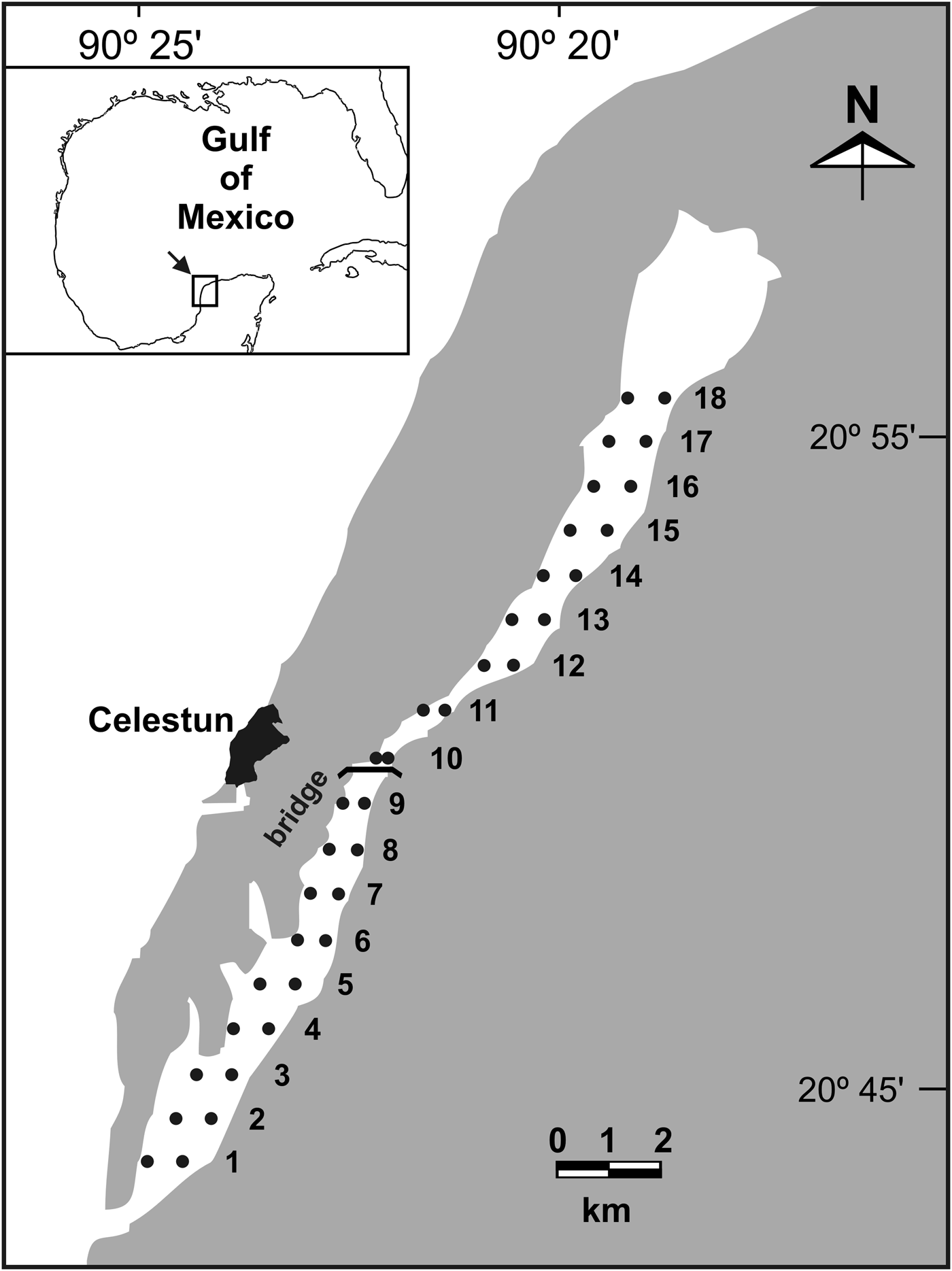
Celestun Lagoon (Mexico) is a tropical estuarine habitat of ~22.5 km long, in the Gulf of Mexico (Figure 1). The substratum of this microtidal shallow lagoon with an almost flat bottom is dominated by SAV beds, mainly composed of the green alga Chara fibrosa (C. Agardh ex Bruzelius) in areas with low salinity (<15), the seagrass Ruppia maritima (Linnaeus) in brackish waters (10–25 m) and the seagrass Halodule wrightii (Aschers) in areas with marine conditions (Chávez et al., Reference Chávez, Garduño and Arreguin-Sanchez1993; Pérez-Castañeda & Defeo, Reference Pérez-Castañeda and Defeo2004; Herrera-Silveira, Reference Herrera-Silveira2006). The lagoon has strong spatial gradients in environmental variables with seasonal fluctuations (Pérez-Castañeda & Defeo, Reference Pérez-Castañeda and Defeo2004). In the present study we assessed spatio-temporal variations in SAV distribution and environmental variables (sediment and water), as well as the role played by these variables in explaining SAV distribution in Celestun Lagoon.
Location of sampling sites (•) along the estuarine habitat of Celestun Lagoon, Mexico. 1–18: distance (km) from the mouth of the lagoon.
MATERIALS AND METHODS
Study area
Celestun Lagoon is located in the north-west of the Yucatan Peninsula (20°45′N 90°25′W) in the Gulf of Mexico. It has an area of 28.14 km2 and is connected to the sea by a 0.46 km wide mouth (Figure 1). It is a microtidal shallow lagoon with flat bottom, a mean depth of 1.2 m and a narrow tidal channel with a maximum depth of 3 m (Pérez-Castañeda & Defeo, Reference Pérez-Castañeda and Defeo2004). Celestun Lagoon is characterized by high and constant turbidity because of continuous sediment resuspension and diffusion of ‘tannins’ from mangroves throughout the lagoon (Pérez-Castañeda & Defeo, Reference Pérez-Castañeda and Defeo2004). As there are no rivers, the spatial salinity gradient is conditioned by groundwater discharges (via freshwater springs in the northern part of the lagoon), tides and climatic seasons (Dry, March to May; Rainy, June to October; and Nortes (fronts), November to February). The Dry season is characterized by little rainfall (0–50 mm month−1) in comparison to the Rainy season (>500 mm month−1). Whereas the Dry and Rainy seasons are characterized by south-west winds <15 km h−1, the Nortes season is affected by strong winds from the north (80 km h−1), little rainfall (20–60 mm month−1) and cool air temperatures (22°C) (Herrera-Silveira, Reference Herrera-Silveira1994).
Sampling and laboratory procedures
We conducted three seasonal sampling surveys during February, April and September 2005, corresponding to the ‘Nortes’, ‘Dry’ and ‘Rainy’ seasons, respectively. We selected 18 pairs of sites from the outer to the inner zone of the lagoon at 1 to 1.5 m depth. Distance between consecutive pair of sites was 1 km (Figure 1). All samplings were carried out under the same conditions (depth and time of day) in order to minimize the effects on sample efficiency associated with sampling conditions. In order to complete each survey during one morning, three teams sampled the lagoon simultaneously.
Four sediment samples were taken in each site with a hand corer (5 cm diameter) to estimate grain size, organic carbon (OC), total nitrogen (TN) and total phosphorus (TP). OC was determined following the methods of Buchanan (Reference Buchanan, Holme and Mcintyre1984), whereas TN and TP were obtained by wet oxidation of the dried sediments with potassium persulphate in basic and acidic conditions, respectively (Parsons et al., Reference Parsons, Maita and Lalli1984; Adams, Reference Adams1990). Grain size was estimated by suspending the sediment and measuring the density with a hydrometer.
Water samples were taken with Van Dorn bottles, stored at 4°C and brought into the laboratory for further analyses. pH was taken with a Beckman Phi-32 pH meter and combined glass electrode (NBS scale). In the laboratory, total suspended solids (TSS) were determined following the methods of Stirling (Reference Stirling1985). The salinity of the filtered water was recorded using a salinometer (Kahlsico RS-9). Ammonium, nitrites, nitrates, phosphates and silicates were quantified using colorimetric techniques (Strickland & Parsons, Reference Strickland and Parsons1972; Parsons et al., Reference Parsons, Maita and Lalli1984) with a Shimadzu 1201 UV/VIS spectrophotometer.
At each site, three replicate SAV samples (0.2 m2 each) were taken, bagged and placed on ice for later analyses. In the laboratory, the SAV was rinsed free of sediment, sorted to species level (Littler & Littler, Reference Littler and Littler2000) and oven-dried for 24 hours to a constant weight at 60°C to determine biomass (dry weight, g m−2). Rhizomes (horizontal stem found underground) were considered for biomass estimations.
Spatial structure: geostatistics
A geostatistical appraisal was performed to examine the spatial structure and distribution of sedimentological and water variables, and SAV biomass (total and specific) along the estuarine–lagoon habitat. Geostatistics focus on the detection, modelling, and estimation of spatial patterns in spatially correlated data (Rossi et al., Reference Rossi, Mulla, Journel and Franz1992). Spatial autocorrelation occurs when samples collected close to each other are often more similar than samples collected farther apart, particularly when the variable sampled is spatially structured (e.g. in patches). Geostatistics usually involve 2 steps (Robertson, Reference Robertson1987): (1) characterizing the spatial structure of the variable by means of a variogram, thus defining the degree of autocorrelation among the data points; and (2) predicting values between measured points based on the estimated degree of autocorrelation. The spatial structure of a dataset is usually described by an empirical variogram, which is basically a plot of the variance or difference between pairs of observations against their distance in geographical space (Wagner, Reference Wagner2003). Variogram parameters are used for interpolating values, using a kriging algorithm that provides an error term for each value estimated, giving a measure of reliability for the interpolations (Robertson, Reference Robertson1987, Reference Robertson2000). In this paper, variographic analysis and punctual kriging were used to characterize the SAV spatial structure and make local predictions. In accordance with the main objective of this study, a one dimensional approach was used. The spatial autocorrelation of these variables was evaluated by semivariance analysis through variograms, which quantify the spatial dependence between them. Changes in semivariance within a variogram represent the rate of deterioration of the influence of a given sample over increasingly remote zones in the study area (Matheron, Reference Matheron1963). To this end, mean values of SAV biomass (total and specific) and sedimentological and water variables were calculated for each pair of sampling sites along the coastal lagoon. The 1-dimensional transects consisted of 18 mean observations measured at a location x defined with respect to its relative distance from the mouth of Celestun Lagoon (1 to 18 km) (Pérez-Castañeda & Defeo, Reference Pérez-Castañeda and Defeo2004). Because variograms tend to decompose at large lag intervals close to the maximum lag interval, the active lag distance used in the variographic analysis was close to 80% of the maximum lag.
A variogram γ(h) was estimated for each one dimensional transect (consisting of 18 mean values of the variable studied) using Matheron's (1965) estimator:
 $$\gamma \lpar h\rpar = \displaystyle{{\sum\limits_{i = 1}^{Nh} {\lsqb Z\lpar x_i + h\rpar - Z\lpar x_i \rpar \rsqb } ^2 } \over {2N\lpar h\rpar }}$$
where Z(xi) is the measured sample value at location xi, Z(xi + h) is another measured sample value separated from xi by a distance h (measured in km), and N(h) is the number of pairs of observations separated by h. Several theoretical models (spherical, exponential, Gaussian and linear) were fitted to the experimental variograms. The models provide the following parameters (Robertson, Reference Robertson1987): (1) the nugget-effect (C 0), which reflects the spatial variability below the minimum lag distance that cannot be modelled with the current sampling resolution (i.e. 1 km in this case); (2) the sill (C 0 + C), which defines the asymptotic value of semivariance; and (3) the range (A 0), defined as the distance over which autocorrelation is present (Cressie, Reference Cressie1991). These parameters allow the proportion of sample variance explained by the spatially structured component C/(C 0 + C) to be estimated. A variable is spatially structured if the proportion of sample variance (C 0 + C) that is explained by spatially structured variance C tends to 1. In this case, the variogram with no nugget variance and the curve passes through the origin. The different variograms were defined as:
Spherical:
 $$\matrix{{\rm \gamma }\left({\rm h} \right)= {\rm C}_0 + {\rm C}\left[1.5\left({\rm h/A}_0 \right)- 0.5\left({\rm h/A}_{\rm 0} \right)^3 \right] &{\rm for }\, {\rm h} \le {\rm A}_0 \cr {\rm \gamma }\left({\rm h} \right)= {\rm C}_0 + {\rm C} &{\rm for}\, {\rm h} \gt {\rm A}_0 }$$
Gaussian:
 $$\gamma \lpar {\rm h}\rpar = {\rm C}_0 + {\rm C\lsqb 1 - exp\lpar \!\!-\!\! h}^2 /{\rm A}_0 ^2 \rpar \rsqb$$
Here, the effective range is given by A = 30.5 A0, which is the distance at which the sill (C + C0) is within 5% of the asymptote.
Exponential:
 $$\gamma \lpar {\rm h}\rpar = {\rm C}_0 + {\rm C\lsqb 1 - exp\lpar \!\!-\!\! h/A}_0 {\rm \rpar \rsqb }$$
With the effective range being A = 3A0, which is the distance at which the sill (C + C0) is within 5% of the asymptote. The sill never meets the asymptote in the exponential or Gaussian models.
The model fitting procedure used the reduced sum-of-squares of the residuals (RSS) to choose parameters for each of the variogram models by determining a combination of parameter values that minimizes RSS for any given model (see details in Robertson, Reference Robertson2000). The coefficient of determination (r2) was also used as an additional indicator of goodness of fit, even though this estimate is not as robust as the RSS for best-fit calculations.
Once spatial dependence had been determined, variogram parameters to interpolate values along each transect for points not measured through punctual kriging (Matheron, Reference Matheron1965) were used. Punctual kriging provides an error term for each estimated value, therefore giving a measure of reliability for the interpolations. Subsequently, kriging values were used to validate the fitted variogram through cross-validation. This procedure is based on the systematic removal of observations from the raw data set, one by one, which were then estimated by kriging. Estimated (E) versus observed (O) values were fitted to a linear regression of the form O = α + βE, and departures from a 1-to-1 line through the origin indicated model inadequacy. The simultaneous F test (Dent & Blackie, Reference Dent and Blackie1979) was used to test the null hypothesis of slope = 1 and intercept = 0. After modelling the spatial autocorrelation and validating the fitted variogram, a transect image of the analysed variable, including observed data, interpolations, and the variance of interpolations, was generated. Interpolation was not carried out in cases where spatial autocorrelation was not detected and only the observed data were plotted to depict any spatial trend. An analysis of covariance (ANCOVA) was performed for salinity and silicates, with season as the main factor, distance as the covariate, and log (salinity or silicates) as the dependent variable. This analysis was restricted to km 2 to 18 in order to fulfil ANCOVA requirements.
Relationship between SAV distribution and environmental variables
Multivariate analysis was used to assess the relative effect of sedimentological and water variables on SAV distribution and biomass. Canonical correspondence analysis (CCA) was chosen for modelling, since gradient length and eigenvalues suggested a unimodal model (Dodkins et al., Reference Dodkins, Rippey and Hale2005). Variance inflation factors (VIFs) were assessed: a high value for the VIF (>20) indicates multicollinearity between variables (Ter Braak, Reference Ter Braak1986) and thus the variable with the highest VIF was removed. This procedure was repeated until all VIF values were <10. Statistical tests were carried out using a Monte Carlo simulation with 499 permutations (Ter Braak & Smilauer, Reference Ter Braak and Smilauer2002). The analysis was performed using the computer program CANOCO 4.5 (Ter Braak & Smilauer, Reference Ter Braak and Smilauer2002).
RESULTS
Spatial analysis
SEDIMENTS
Organic carbon was always spatially structured (Table 1). In Nortes and Rainy seasons the spatial structure was best characterized by a spherical variogram, and in the Dry season by a Gaussian variogram (Figure 2; Table 1). OC variograms revealed a high and stable spatial structure (C/(C 0 + C) >94%). The distance of spatial influence, A0 (interpreted as patch size), was 10.26 km, 10.48 km and 3.55 km in the Nortes, Dry and Rainy seasons, respectively (Table 1). In the three climatic seasons OC tended to show higher concentrations between sites 3 and 6, decreasing towards the inner zone of the lagoon. The Dry season presented the lowest OC concentrations (Figure 3).
Theoretical variograms fitted for sediment and water variables, and submerged aquatic vegetation biomass in: (A) Nortes, (B) Dry and (C) Rainy seasons. Details of variogram models are shown in Table 1. Mean values of each variable along the one dimensional transect were used. Note the different scales of X and Y axes. Spatial autocorrelation was not detected in some cases (not shown).

Transect images for each season ((A) Nortes, (B) Dry and (C) Rainy) generated with punctual kriging, showing observed (•) and predicted mean (continuous lines) ± SD (dotted lines) biomass for environment variables in sediment water and seagrasses Halodule wrightii and Ruppia maritima, green alga Chara fibrosa, and total submerged aquatic vegetation along the estuarine habitat. Note different scales of Y-axes.

Parameters and goodness of fit criteria for variographic and cross-validation analyses of punctual kriging estimates for sediment and water variables (TP, total phosphorus; TN, total nitrogen) and submerged aquatic vegetation (SAV) species (Halodule wrightii, Ruppia maritima, Chara fibrosa and total vegetation) in N, Nortes, D, Dry, R, Rainy seasons, in Celestun Lagoon. Mean values of each variable along a one dimensional transect were used. Sphe (spherical), Gauss (Gaussian) and Exp (exponential); C0, nugget effect; C0 + C, asymptotic semivariance; A0, distance (km) over which autocorrelation occurs; % spatially structured component [C/(C0 + C)]; r2 coefficient of determination; RSS, reduced sum of squares; Bias: simultaneous F statistic for slope = 1 and intercept = 0; in all cases P > 0.05. Only those cases with spatial structure are shown.

Total phosphorous concentrations only presented a marked spatial structure during the Dry season, and were best modelled by a spherical variogram, which presented a high and stable spatial structure and a spatial autocorrelation distance of 8.41 km (Table 1; Figure 2). The transect image presented the highest concentrations at site 2, gradually decreasing to their lowest between sites 7 and 12, increasing again between sites 13 and 16 (Figure 3).
Total nitrogen structure was best represented by a spherical variogram during Nortes, with a high and stable spatial structure and a spatial autocorrelation distance A0 of 4.56 km (Table 1; Figure 2). The transect image displayed the highest concentrations between sites 3 and 6 (Figure 3). No structuring was displayed in Rainy and Dry climatic seasons.
Sediment grain size did not display spatial structure, but decreased linearly from the mouth of the lagoon towards the inner zone. The ANCOVA performed with climatic season as main factor, distance (D) (2 to 18 km) as the covariate and grain size as the dependent variable, showed that for the same D, grain size significantly varied between seasons (F2,48 = 8.90; P < 0.01), with the lowest values in the Rainy season (Tukey test: P < 0.001).
WATER
Silicates, salinity and pH showed clear spatial gradients along the lagoon, and a lack of spatially organized internal structure (Figure 4). Silicate concentration decreased from the inner zone seawards because of an influx of groundwater in the inner zone of the lagoon (Figure 4A). This continuous spatial gradient of silicates (Si) followed an exponential function of the form: Si = aе (bD) where a and b are significant parameters (P < 0.01). Silicates varied between seasons (ANCOVA: F2,48= 107.06), being significantly higher in the Rainy season (207.28 to 395.88 µM) than in Nortes (61.65 to 305.98 µM) and Dry (18.18 to 214.90 µM) seasons (Tukey test, P < 0.0001).
Seasonal variations in silicates, salinity and pH along Celestun Lagoon. Data points correspond to mean values over 1 to 18 km. Exponential decay models fitted for each season are shown.

Salinity (S) decreased from the seaward end (site 1) to the innermost zone (site 18) of the lagoon, following a monotonically decreasing exponential function of distance (D) from the mouth of the lagoon of the form: S = aе (−bD), where a and b are significant parameters (Figure 4B). Salinity significantly differed between seasons (ANCOVA: F2, 50= 164.13), with the highest values in the Dry season (28.02 to 37.40) and the lowest ones in the Rainy season (8.33 to 22.43) (Tukey test, P < 0.001).
The pH linearly increased with distance (D) from the mouth of the lagoon (Figure 4C), following the model pH = a + bD, where a and b are significant parameters (P < 0.01). The pH significantly differed between climatic seasons (ANCOVA: P < 0.01), being higher in the Rainy season than in Nortes and Dry seasons (Tukey test, P < 0.0001).
Ammonium was spatially-structured in the Nortes and Rainy seasons (Table 1). The structure was best characterized by spherical variograms with a stable spatial structure C/(C0 + C) ≥99%. The spatial influence distance, A 0 was 2.86 and 2.62 km in the Nortes and Rainy seasons respectively (Table 1; Figure 2), where ammonium concentrations were highest at sites 17 and 18 (Figure 3).
Nitrates were highly spatially structured (>95%) in all three climatic seasons (Table 1), and best characterized by spherical (Nortes and Dry seasons) and Gaussian (Rainy season) variograms (Figure 2). A0 was 9.58 km for the Nortes season, 9.52 km for the Dry season and 7.83 km for the Rainy season (Table 1; Figure 2). The transect image showed the highest concentrations between sites 6 and 15, particularly during the Rainy season (Figure 3).
SUBMERGED AQUATIC VEGETATION (SAV)
Halodule wrightii was spatially structured in Nortes and Rainy seasons and best characterized, respectively, by exponential and spherical variograms (Table 1). Variograms showed that spatially structured component C/(C 0 + C) was always ≥50%. The spatial influence distance (A 0) was 2.68 km (Nortes) and 1.36 km (Rainy) (Table 1; Figure 2). In Nortes, Halodule wrightii presented a continuous distribution with no definite alongshore pattern, being absent from km 15 to inner waters (Figure 3). In the Rainy season, H. wrightii showed a continuous distribution along the lagoon, with the highest biomass at sites 3, 4, 10 and 14. Ruppia maritima presented spatial structuring in Nortes and Dry seasons, being modelled, respectively, by spherical and exponential variograms [C/(C0 + C) > 85%]. The spatial influence distance A0 was 1.54 km in Nortes and 2.76 km in the Dry season (Table 1; Figure 2). In Nortes, R. maritima biomass was highest between km 12–13 and 15–16, while in the Dry season peaked between sites 11 and 16, with a biomass four times greater than in Nortes (Figure 3). Chara fibrosa presented spatial structure in the Rainy season and was best represented by a spherical variogram [C/( C0 + C) > 90%] and A0 = 6.3 km (Table 1), and its highest biomass was found between sites 13 and 17 (Figure 3). Total SAV was best represented in Nortes and Dry seasons by exponential variograms, and in the Rainy season by a spherical variogram with a structure ≥90% and A0 values of 2.63 km in Nortes, 1.91 km in the Dry season and 6.12 km in the Rainy season (Table 1).
Relationship between environmental variables and SAV
SEDIMENT
The first CCA axis explained most of the variance in sediment variables (OC, TP, TN and grain size) as follows (Table 2): Nortes 49%, Dry 53% and Rainy 45%. Significant eigenvalues were 0.539 in the Dry season and 0.455 in the Rainy season. The variance explained (marginal effects) by TP, TN and grain size was small (≤13.87%) in the three seasons (Table 3). OC was significant in the Dry and Rainy seasons (conditioned effect: P< 0.05), and best structured the SAV biomass: the variance explained in the Dry season was 24.09% and in the Rainy season was 36.26% (Table 4).
Canonical correspondence analysis of sediment and water variables in Celestun Lagoon for submerged aquatic vegetation species. Eigenvalues of the first two axes, variance explained, and F and P values for the first axis are detailed for each climatic season.

Canonical correspondence analysis variance partitioning analysis explained by each variable (sediment and water) individually (marginal effects) in three climatic seasons in Celestun Lagoon.

–, absent values because of colinearity.
Environmental variables (marginal effects = λ1) in canonical correspondence analysis for sediment and water variables of three estuarine-lagoon species of submerged aquatic variation in Celestun Lagoon, in N, Nortes, D, Dry and R, Rainy seasons. Total inertia = 1.47. *P < 0.05. R**, silicates against salinity because of colinearity. Abbreviations of variables are detailed in Figure 5.

In Nortes, the ordination diagram for sediment variables showed that grain size was the most important explanatory variable of SAV variation. Abundance of H. wrightti was negatively associated with grain size, R. maritima with OC, and Ch. fibrosa with TN and TP (Figure 5A). For the Dry season, SAV variation was mostly related to OC. Ruppia maritima exhibited a positive association with grain size, and a negative association with OC, TP and TN (Figure 5B). For the Rainy season (Figure 5C), OC best explained variations in SAV. SAV biomass at sites 15–18 followed a clear association with Ch. fibrosa, which in turn was negatively associated with OC, TN and TP. The distribution at sites 6–13 showed association with R. maritima.
Canonical correspondence analysis triplot variation in submerged aquatic vegetation (SAV) biomass and environmental variables in Celestun Lagoon in three climatic seasons: (A) Nortes, (B) Dry and (C) Rainy; SAV species (▴), environmental variables (arrows) and km (•). SAV species: Halodule wrightii, Ruppia maritima and Chara fibrosa. Variables estimated in the sediment: organic content (OC), total nitrates (TN), total phosphorous (TP) and grain size (GRA). Variables estimated in water: ammonium (NH4+), nitrates (NO3−), phosphates (PO4−3), salinity (Sal), silicates (Si), pH and total suspended solids (TSS).

WATER
The first axis of the CCA explained 91% of the variance in Nortes, 64% in Dry and 54% in Rainy seasons. The relationships between response and explanatory variables were significant for the three climatic seasons (Monte Carlo test: P < 0.05), with eigenvalues of 0.56, 0.64 and 0.54 respectively (Table 2). Nitrites (all seasons), silicates (Nortes and Dry seasons) and salinity (Rainy season) were omitted because collinearity > 10. Individually, nitrates, phosphates, silicates and TSS variables in the three seasons explained <9%. Ammonium (Nortes); pH, salinity and TSS (Dry season); and TSS (Rainy season) significantly (conditioned effect: P < 0.05) explained spatial variations in SAV biomass (Table 3). CCA for Nortes showed that nitrates, phosphates and salinity best explained distributional patterns of SAV, whereas salinity and TSS were the most important variables for the Dry and Rainy seasons, respectively (Figure 5).
DISCUSSION
Geostatistical analysis revealed autocorrelation in SAV samples, and thus variographic analyses successfully explained the spatial structure of SAV. The biomass of H. wrightii, R. maritima and Ch. fibrosa displayed wide variations in spatial structure between climatic seasons, both in abundance and patch size (A0) that in most cases varied in more than 100%. The green alga Ch. fibrosa presented a strong spatial structure in the Rainy season and almost disappeared in Nortes and Dry seasons (salinity >34), because it is mainly associated with low salinity conditions (Pérez-Castañeda & Defeo, Reference Pérez-Castañeda and Defeo2004; Herrera-Silveira, Reference Herrera-Silveira2006). By contrast, R. maritima was spatially structured and its biomass was particularly highest in the Dry season, taking advantage of high salinity levels (>30) (Pérez-Castañeda & Defeo, Reference Pérez-Castañeda and Defeo2004; Herrera-Silveira, Reference Herrera-Silveira2006), even though it can colonize marine, estuarine and freshwater habitats (Lazar & Dawes, Reference Lazar and Dawes1991). Finally, H. wrightii was spatially structured in Nortes and Rainy seasons, with low biomass and intermittent occurrence from sites 1 to 14. Similar patterns of spatial structure have been detected in other seagrasses, also using geostatistical techniques (Zupo et al., Reference Zupo, Mazella, Buia, Gambi, Lorenti, Scipione and Cancemi2006). Variations in persistence of a spatial structure in plant communities through time could occur in the forms of (Wagner, 1993): (1) single-species aggregation and dispersion patterns; (2) distance-dependent interactions between species; and (3) the response to the spatial structure of environmental conditions. In this paper, spatio-temporal trends in abundance and patch size of the three SAV species could result from a combination of vegetative expansion and a differential response to the spatial structure of environmental conditions, notably salinity. In this context, experimental results showed that R. maritima has a competitive advantage over other seagrasses (e.g. H. wrightii) by having broader tolerances to salinity and temperature and an earlier annual growth cycle (Lazar & Dawes, Reference Lazar and Dawes1991). Moreover, vegetation maps of the lower Laguna Madre prepared from long-term surveys showed a decrease in cover by H. wrightii, concurrently with an increase in other seagrass species, in deeper parts of the lagoon (Quammen & Onuf, Reference Quammen and Onuf1993). Turbidity caused by maintenance dredging and reductions in salinity maxima were suggested by these authors as critical drivers that have limited expansion rates of seagrasses into suitable habitats. This is of utmost importance, given that hypo- and hyperosmotic conditions could inhibit photosynthesis in seagrasses (Touchette, Reference Touchette2007). Thus, the differential tolerance among species to salinity variations, which characterizes estuarine systems such as Celestun Lagoon, could explain spatio-temporal trends in SAV biomass.
Multivariate ordination techniques were also useful to describe multispecies SAV responses to environmental factors. The spatial distribution of the SAV biomass along the estuarine habitat was best explained by the salinity gradient of the lagoon, whereas seasonal variations in biomass (total and discriminated by species) were best explained by OC, salinity and TSS. Concerning sediment variables, OC best explained spatial gradients in SAV biomass for Dry and Rainy seasons. This trend could be explained by a feedback process: SAV and microphytobenthos supply significant quantities of organic material (Kristensen et al., Reference Kristensen, Bouillon, Dittimar and Marchand2008) and, at the same time, organic material (carbon) contributes to SAV production (Koch, Reference Koch2001). OC showed highest concentrations between sites 3 and 9, where H. wrightii biomass was also highest, decreasing towards the inner zone of the lagoon.
Concerning water variables, ammonium in Nortes, salinity in the Dry season and TSS in the Rainy season mostly explained spatial variations in SAV biomass. Particularly, the strong salinity gradient along Celestun Lagoon was the most prominent feature of this ecosystem, exponentially decreasing from the mouth to the inner zone. A 0 was greater in nitrate than in ammonium, reflecting a higher stability in the former. Average nitrate concentrations in the three climatic seasons were around the same value reported by Herrera-Silveira (Reference Herrera-Silveira2006) for this lagoon (10 µM) and others (<80 µM) (Soetaert & Middelburg, Reference Soetaert and Middelburg2009; del Pozo et al., Reference del Pozo, Fernández-Aláez and Fernández-Aláez2010). In Yucatan, groundwater discharges are rich in nitrates (Herrera-Silveira, Reference Herrera-Silveira1994), including Celestun Lagoon (Herrera-Silveira, Reference Herrera-Silveira2006). Concerning ammonium, Herrera-Silveira (Reference Herrera-Silveira2006) obtained reference values of 8 µM in the lagoons of the Yucatán Coast, 12 µM in Celestun Lagoon, and the average for this kind of ecosystem is between 5 and 10 µM (Contreras et al., Reference Contreras, Castañeda, Torres and Gutiérrez1996). Higher values obtained in the present study during Nortes (16.5 µM), Dry (23.4 µM) and Rainy seasons (13.3 µM) could be related to organic matter decomposition processes originated from the SAV and the mangrove forest that surrounds the lagoon (Zaldívar et al., Reference Zaldívar, Herrera-Silveira, Coronado-Molina and Parra2004). In addition, these values could indicate an increase in eutrophic conditions of the system, reflecting a deterioration of the habitat that could be mainly ascribed to an exponential increase through time in motor boat traffic and bottom trawl fishing, which fragments and unpins the SAV and increases the amount of decomposition material. In this context, seagrasses could disappear and even be displaced by e.g. seaweeds, particularly in cases with eutrophication, causing regime shifts where green meadows and clear waters are replaced with unstable sediments, turbid waters and hypoxia (Quammen & Onuf, Reference Quammen and Onuf1993; Thomsen et al., Reference Thomsen, Wernberg, Engelen, Tuya, Vanderklift, Holmer, McGlathery, Arenas, Kotta and Silliman2012). Increased deposition of fine-grain organic particles can also affect SAV growth either by increasing porewater nutrients or by producing phytotoxic reduced sulphur compounds (Kemp et al., Reference Kemp, Batuik, Bartleson, Bergstrom, Carter, Gallegos, Hunley, Karrh, Korch, Landwehr, Moore, Murray, Naylor, Rybicki, Stevenson and Wilcox2004 and references therein).
Marked seasonal differences in water variables (e.g. salinity in the Dry season and TSS in the Rainy season) could also determine differences in the amount of variance explained by multivariate techniques in relation to SAV abundance. Estuaries are highly susceptible to climate forcing (Kimmel et al., Reference Kimmel, Miller, Harding, Houde and Roman2009), and one of these effects is the annual timing and magnitude of freshwater flow via underground discharges: the scarce rainfall in the Dry season makes the habitat more saline. On the other hand, SAV can maintain clear water through the reduction of nutrients (Kemp et al., Reference Kemp, Batuik, Bartleson, Bergstrom, Carter, Gallegos, Hunley, Karrh, Korch, Landwehr, Moore, Murray, Naylor, Rybicki, Stevenson and Wilcox2004). In the Rainy season, TSS concentration became lower and at the same time SAV biomass was the highest of the three climatic seasons. In this way, within-year variations in climatic conditions drive ecosystem responses (Lehman, Reference Lehman2004).
In summary, the salinity gradient was the most important factor determining the spatial distribution of SAV along the estuarine lagoon. Other variables of importance were sediment OC and grain size, as well as water salinity and TSS. Their relative contribution varied seasonally. In this case, salinity could be considered as a key factor shaping patterns in occurrence, abundance and spatial structure of seagrass beds reinforcing the notion of seagrasses as sensitive species to spatio-temporal variations in estuarine conditions.
ACKNOWLEDGEMENTS
This work is part of the PhD thesis of A.M. Burgos-León at CINVESTAV Mérida. Financial support from Consejo Nacional de Ciencia y Tecnología (grant to A.M.Burgos-León) is acknowledged. We thank the Fishery and Chemical Laboratory staff for help during field and laboratory activities.



