One of the key criteria in evaluating liberal democracies is the extent to which government actions are responsive to public opinion. In empirical work, this has often been assessed by examining the degree of congruence between government policy and the position of the median citizen or voter on the left-right dimension. The results have been decidedly mixed. Whereas some studies have highlighted the extent to which “ideological congruence” actually exists in extant democracies (McDonald and Budge Reference McDonald and Budge2005; Budge et al. Reference Budge, McDonald, Pennings and Keman2012), others have found that two-sidedness or bilateralism is the more prevalent pattern, not just in terms of the party compositions of governments but also in terms of their policy stances (Warwick Reference Warwick2010; Warwick Reference Warwick2011a; Warwick Reference Warwick2011b).Footnote 1
The principals involved have debated this issue extensively (Best, Budge and McDonald Reference Best, Budge and McDonald2012; Warwick Reference Warwick2012) and it is not the purpose of this paper to pursue the matter further. Instead, the goal is to start from a premise on which both sides agree—that the left-right policy stances of governments do not approximate the left-right median in many cases (Best, Budge and McDonald Reference Best, Budge and McDonald2012)—and ask the question: What accounts for these instances of divergence from centrism in government policy? More specifically, which factors or considerations lead governments to be composed mainly or entirely of parties located on one side of center on the major dimension of political competition and to adopt policy stances that diverge from the center?
Perhaps owing to the sway held by the idea of ideological congruence, this question has seldom been addressed in the recent literature. Nor do earlier works provide much guidance. Duverger’s (Reference Duverger1954, 239–46) seminal treatise on political parties saw politics as inherently dualistic, while Sartori’s (Sartori Reference Sartori1976, 131–92) equally influential work on party systems qualified this judgment principally by limiting it to systems where ideological polarization is not high. Given that appeals to presumed inherent tendencies hardly satisfy as explanations, what else can be proposed?
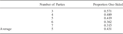
To begin with, we must acknowledge that some level of “one-sidedness” may appear without any systematic cause. Imagine a parliamentary system with three parties that compete, at least partly, in left-right terms. Imagine further that each party can be categorized as either on the left or the right of the spectrum, with at least one party on each side (otherwise the left-right distinction would be meaningless). There are seven possible governments that might be formed in this scenario, of which four would be one-sided, that is, composed entirely of parties from one side of the spectrum. Hence, if government formation were purely random, we would expect a one-sided government to emerge in 4/7th or 57.1 percent of formation opportunities. Table 1 shows the rates for party systems ranging from three to seven parties. The rates range from 57.1 to 31.5 percent. They would be lower still for party systems with more than seven parties, but higher (66.7 percent) for two-party systems. Thus, under random formation, we would expect a substantial proportion of governments to be one-sided in any system that has sides.Footnote 2
Random Production of One-Sided Governments

Note: Calculations assume that party systems can be divided such that at least one party is on each side of the dividing line.
If real-world outcomes mirrored these percentages, we might conclude that the government formation process must be essentially random and that no tendency toward dualism exists. But they do not. In Armingeon et al.’s (Reference Armingeon, Laura, David and Sarah2014) Comparative Political Data Set (CPDS), for example, about 63 percent of the nearly 1000 governments in 23 countries (excluding caretaker and technocratic governments) are one-sided. Not only is this rate is well above the levels of one-sidedness reported in Table 1, but it is almost certainly an under-estimate. This is because the authors classify parties as left, right, or “centrist,” which means that any government containing a party considered to be centrist, such as a Christian Democratic party, cannot be classified as one-sided. This includes, for example, Germany’s many Christian Democrat/Free Democrat governments, even though they clearly represented one side of the basic divide that has characterized most of postwar German politics.
Given that actual levels of bilateralism exceed what a totally random process would yield, what else might be involved? One possible factor is the rules of the game. As Golder, Golder and Siegel (Reference Golder, Golder and Siegel2012, 430) have pointed out, government formation in parliamentary systems is bound by two constitutional constraints: all governments must be supported (at least implicitly) by a parliamentary majority (as well as by their member-parties) and there is always an incumbent government. Thus, contra the calculations of Table 1, all possible governments are not equally likely; only those that are majority-preferred to the incumbent government are viable.
To speak of some potential governments as being majority-preferred to others raises the issue of what parties want. A common assumption is that they seek both cabinet portfolios and policy proximity (i.e., governments whose policy positions are located as close as possible to their own policy positions). Do these preferences, in conjunction with the Golder et al.’s constitutional constraints, influence the level of one-sidedness? What about other considerations that go into the government formation process, such as constraints on how policy influence or cabinet portfolios are divided up?
Another factor that might be relevant is the way in which voters and parties are distributed in the policy space. Thus, a system in which voters and parties are relatively spread out on the left-right dimension may see more votes funneled to non-centrist parties, which in turn might favor the formation of non-centrist or one-sided governments. Needless to say, this or any other hypothesized relationship may be modified by the extent to which the left-right dimension matters to voters and parties (vis-à-vis other dimensions).
Voters may play a role in fostering one-sidedness beyond that which may follow from the distribution of their policy preferences in the policy space. One such way is through the effects of “valence” on their vote choices. Although the concept of valence was originally introduced by Stokes (Reference Stokes1963) to reference a particular type of policy issue (one in which judgments of competence distinguish the various candidates or parties), recent work has tended to disengage the concept from policy entirely, so that valence often refers simply to generally held beliefs about candidate or party quality (Laver and Sargenti Reference Laver and Sargenti2012, 184). But it is still possible that positioning enters indirectly in the sense that, in any given election, one side of the political spectrum may be the net beneficiary of favorable valence judgments. If large enough, a net valence advantage for one side over the other in an election might easily enhance the prospects of that side forming the next government. Recently, I reported just such a relationship in the Comparative Study of Electoral Systems (CSES) (2003–2013) data (Warwick Reference Warwick and Druckman2016).
Another way in which voters might foster one-sidedness is by favoring parties that espouse more extreme positions than their own. Such behavior may seem unlikely, but it is implied in some influential voting models. The most recent of these is Kedar’s (Reference Kedar2009) compensational model of voting, which sees voters choosing more extreme parties because of the impact those choices would have on expected policy outcomes. If it is true that voters favor more extreme parties, it may promote one-sidedness not just by encouraging parties to avoid the center but by giving parties that do so more support and hence greater bargaining strength in coalition negotiations.
Since actual government formations are a complex interaction of factors, perhaps including but certainly not limited to the ones mentioned above, it can be difficult to isolate specific causal effects with real-world data. In some cases, it is impossible because of a lack of variability. For instance, there may be few parliamentary systems in which policy proximity does not strongly motivate vote choices or coalition behavior. For certain hypotheses, data collection presents a further obstacle. While the extent of compensational voting may vary across elections sufficiently to test the hypothesis that it enhances non-centrist outcomes, the task of assessing its extent in a sufficiently large number of elections would be quite daunting.
This study therefore undertakes an exploration of possible influences on the degree of non-centrism or one-sidedness in government formations through simulation experiments (computational modeling). This methodology is useful not just when variables are difficult to measure or lacking in variability, but whenever formal modeling has not captured the precise way in which outcomes are produced. It is especially valuable for the study of “emergent behavior,” that is, macro-level phenomena that are not “hard-coded at the micro-level, such as when a market computes the price where supply equals demand even though no one is trying to compute the market price” (Page Reference Page1999, 36). Bilateralism is one such phenomenon: it appears to emerge even though the micro-agents—voters and parties—probably have much more narrowly focused goals in mind.
The software created for these experiments extends Golder, Golder and Siegel’s (Reference Stokes2012) “zero-intelligence” model to provide some “intelligence” to the government formation process, as well as numerous other features. In so doing, it allows for all of the factors mentioned above—voter and party distributions and motivations, policy space dimensionality, constraints on government formation, and so forth—to be manipulated in order to explore possible effects on government compositions and policy stances. Because these experiments use imagined rather than real-world data, the outcomes of these experiments cannot tell us what actually fosters non-centrism in the real world. Instead, the goal is to reveal some of the factors that might be conducive to that end and thus serve as a guide to future empirical research on this neglected topic.
In the next section, the software is introduced and evaluated. The following section presents the results, beginning with the effects of various features of the electoral environment, followed by the impact of constraints on the government formation process, and finally by the consequences of valence-based and compensational voter motivations. The conclusion draws implications from these experiments for future research.
A NEW MODEL OF GOVERNMENT FORMATION
The reference model for this investigation is Golder, Golder and Siegel’s (Reference Golder, Golder and Siegel2012) “zero-intelligence” model of parliamentary government formation, hereafter referred to as the GGS model. The term “zero-intelligence” was employed to denote the fact that within the two constitutional constraints noted above—that an incumbent government always exists and that any replacement must have majority parliamentary support—the simulated government formation process is essentially random. In brief, it unfolds as follows. The electorate consists of voters whose ideal points are uniformly distributed in a two-dimensional policy space. The parties (at least three) are randomly distributed in the space and voters vote according to proximity. Perfect proportional representation translates these votes into legislative seat shares. After an election, each party offers a government proposal, which consists of a combination of three randomly chosen elements: a set of parties to be included in the government (always including itself), a policy position for the government, and a distribution of cabinet portfolio shares among government parties. Parties, which value a combination of proximity and portfolios, evaluate each proposal against the status quo government. Any proposal that is strictly preferred to the status quo by all potential members as well as by a legislative majority draws the attention of the head of state. If it is the only such proposal, the head of state installs it as the new government. If more than one proposal does, the head of state chooses one of them at random. If none does, the process is repeated (up to 100 times, as required).
No tractable analytic solution exists for this model, but the Markov process defined above is ergodic, which implies that all output parameters will be draws from unique limiting distributions (Golder, Golder and Siegel Reference Golder, Golder and Siegel2012, 434). To ensure that these limiting distributions are reached, each election is followed by 2500 government formations; the 2500th formation is taken as the government. An election plus this bargaining sequence constitute a “run”, and the number of parties, their positions, and the relative weight they give to portfolios versus policy vary randomly across runs. The entities of interest for Golder et al. were certain aggregate features of a set of runs, such as the distribution of government types (single-party minority, minority coalition, minimal winning coalition, etc.), the relationship between legislative size and cabinet seat shares, and the amount of time (number of attempts) it takes to form a government. They were able to show that these features of the experimental results resemble their real-world counterparts remarkably closely.
The creators acknowledge that this model does not embody an accurate understanding of the government formation process; instead, they see it as “a ‘null’ model …, a baseline from which other models could proceed” (Golder, Golder and Siegel Reference Golder, Golder and Siegel2014, 880). The software developed for the present paper, the Elections and Governments Program, cannot claim to provide completeness, either, but it does attempt to move things much further in that direction. The key changes for the purposes of this paper are as follows.Footnote 3
The first change relates to the ways in which the policy space is characterized. The program allows for one or two policy dimensions, whose relative salience to voters and parties may be set to a fixed value or varied randomly across runs. The program also allows for voters and/or parties to be distributed in the policy space according to uniform or (truncated) normal distributions; for the latter, the parameters again may be fixed or allowed to vary randomly.
A second area of change concerns the motivations of voters. Voters may vote on the basis of proximity alone (using a city-block metric), but they may also allow valence considerations to enter their utility calculations. Parties may be attributed valence assessments based on a uniform distribution (which make them unrelated to position) or a normal distribution (which will provide centrally located parties with higher valence scores). Again, the parameters of the latter can be fixed or allowed to vary across runs. Similarly, the relative salience given to proximity versus valence can be fixed or allowed to vary. Party valences may also be individualized for voters by making them partially dependent on the distance between voter and party, an effect for which recent research (Zakharova and Warwick Reference Zakharova and Warwick2014) provides empirical support. Lastly, voters may follow the compensational logic outlined by Kedar (Reference Kedar2009), in which they choose the party that will move anticipated government policy closest to their own position. Kedar offers three alternatives for calculating anticipated policy: the weighted mean position of all parties in the legislature, the weighted mean of government parties only, or some combination of both. Since voters have no expectation concerning which parties will ultimately end up in government following the 2500-stage negotiating process, the program implements the first option. As in Kedar’s analyses, voters may also vote according to a weighted combination of proximity and compensationalism, with the relative weights fixed or randomly varying across runs.
The final area of change concerns the kinds of governments that may be proposed. The zero-intelligence model has been criticized for the assumption that parties have no preferences among proposals that beat the status quo, which is rather unrealistic (Martin and Vanberg Reference Martin and Vanberg2014). We lack a well-confirmed model of government formation upon which to base a “full-intelligence” alternative,Footnote 4 but it is still possible to add some “intelligence,” or at least some realism, to the process. One such step would be to stipulate that any proposal must offer the weighted mean position of its cabinet parties on each dimension as the government’s policy position on that dimension. The appropriateness of this constraint is difficult to establish empirically, but there is some evidence that it provides at least a reasonable proxy for actual government policy (Warwick Reference Warwick2011b). In fact, its plausibility is such that innumerable studies (including Kedar Reference Kedar2009) have used it as their measure of government position. Another constraint would be that proposals must offer an allocation of portfolios among cabinet parties that is proportional to their seat contributions. This stipulation follows the very close relationship that has been shown to exist between the two traits in real-world parliamentary systems (Browne and Franklin Reference Browne and Franklin1973; Warwick and Druckman Reference Warwick2006), a property sometimes referred to a “Gamson’s Law.”
How far do these refinements of the government selection mechanism take us? Clearly, not to a state of perfect prediction, but perhaps to outcomes that represent draws from distributions of reasonably likely outcomes.Footnote 5 This cannot simply be assumed, of course; it needs to be tested. One type of test is to determine if known relationships emerge from the simulation results. In the present context, the most important such relationship is that between vote choice and government policy. In a recent analysis of CSES data, I found a substantial linear connection between the mean left-right vote choice in elections and the left-right position(s) of the government(s) that followed them (Warwick Reference Warwick and Druckman2016).Footnote 6 To the extent that the constraints on government proposals suggested above enhance verisimilitude, one would expect the governments that emerge to show a similar degree and type of responsiveness to aggregate voter opinion.
Two sets of simulation runs were therefore conducted to test this expectation. The exact specifications for these (and all other) simulation sets (SS) are given in the Online Appendix, but, in brief, they are as follows. A SS consisted of 5000 elections in which party systems of three, four, five, six and seven parties were equally represented (thus, 1000 three-party systems, 1000 four-party systems, and so on). The policy space for each election contained two independent dimensions of range [0, 1] in which voters and parties were distributed normally according to specifications that are reasonably consonant with real-world data.Footnote 7 To capture the idea of a dominant left-right dimension, the first dimension was given twice the weight of the second in both voter and party utility calculations. In each election, voters chose by proximity alone, albeit with some random error. The government formation stage then proceeded as in the GGS model. The only specification that differs across the two sets of simulations is the constraints placed on government proposals: in the first run, the “zero-intelligence” specification was used; in the second, the two formation constraints presented above were applied.
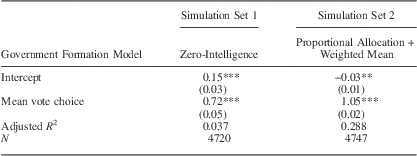
The relationships between mean vote choice and government position on the dominant first dimension in the two SSs are shown in Table 2. Each regression is based on slightly less than 5000 simulation runs because of the occasional occurrence of “lopsided” party systems, that is, those in which all parties were located on the same side of center, which were discarded as unrealistic. The first column reports the results using the zero-intelligence model (SS 1). They show that mean vote choice and government position are positively related, but that the linkage between the two is very weak (adjusted R 2=0.037), which is consistent with Martin and Vanberg’s (Reference Martin and Vanberg2014) criticism of the model. This changes dramatically, however, when government positions and portfolio allocations are constrained to be proportional to government party sizes (SS 2). Mean vote choice is now quite strongly related to government position on the dominant dimension (adjusted R 2=0.288). Visual inspection indicates that the relationship is essentially linear, as hypothesized.
Responsiveness Under Two Models of Government Formation
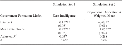
Note: Each column reports the results of regressing government position on the first dimension on mean vote choice on that dimension across a set of 5000 simulations produced using a particular model of government formation, with standard errors in brackets. Simulated party systems in which all parties were located on one side of center were excluded.
*p<0.10, **p<0.05, ***p<0.01.
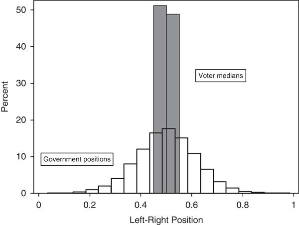
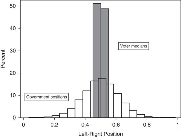
The second or PAWM (proportionally allocated+weighted mean) specification produces a much more realistic indication of responsiveness, but does it also produce the striking difference between the centrality of voter opinion and the non-centrality of government positions that motivates this investigation? In other words, does it show responsiveness to be limited in the same manner as in the CSES data (Warwick Reference Warwick and Druckman2016)? This question is addressed in Figure 1, which shows the distributions of voter medians and government positions on the first dimension (our simulated left-right dimension). Government positions are clearly much less center-concentrated than voter medians, a pattern which closely resembles that produced using the CSES data.
Voter medians and government positions under a proportionally allocated, weighted mean model of simulated government formations Note: The data are from Simulation Set 2, with the first dimension taken to be the left-right dimension. N=4747.
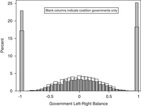
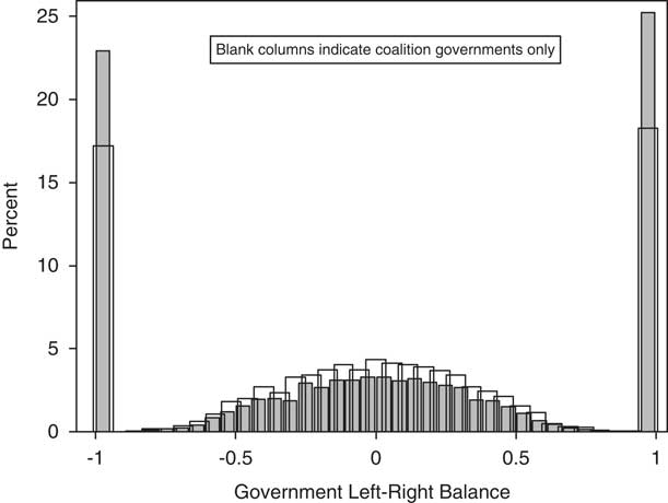
A further test would be to consider the degree of one-sidedness in government compositions that underlies this relative spread of government positions. The simplest indicator would be the proportion of one-sided governments, but this is a rather blunt instrument: it makes no distinction between a government composed almost but not entirely from one side of the spectrum and a government that represents both sides equally. A better approach would be to calculate the difference between the proportion of government seats held by right-of-center parties and the proportion held by left-of-center parties. With this measure, a government whose seat share is 90 percent right-wing would receive a score of “0.8” (0.9–0.1), reflecting the idea that it is almost but not entirely right-wing, whereas a perfectly balanced government would receive a score of “0” (0.5–0.5). This variable, denoted Government Left-Right Balance, will thus range continuously from “−1” for entirely left-wing governments to “1” for entirely right-wing governments, with scores in between representing varying degrees of imbalance to one side or the other.
Figure 2 plots the distribution of this variable for the same simulated data (the PAWM set). The distribution is striking both for the high proportion of entirely one-sided governments (even when single-party governments are excluded) as well as for the relative dearth of balanced governments in the center. This distribution, too, resembles closely its real-world analog as calculated from the CSES data (Warwick Reference Warwick and Druckman2016).
Government left-right balance under a proportionally allocated, weighted mean model of simulated government formations Note: The data are from Simulation Set 2, with the first dimension taken to be the left-right dimension. N=4747.
Thus, it appears that the modeling exercise undertaken here is capable of reproducing, grosso modo, the real-world one-sidedness or bilateralism in government compositions and policy that is the subject of this investigation. In the next section, we turn to the factors that may influence the extent of the phenomenon in this simulated world.
SIMULATING THE IMPACT OF CONTEXTUAL AND MOTIVATIONAL FACTORS ON BILATERALISM
We saw earlier that even a totally random and constraint-free government formation process would produce sizeable levels of one-sidedness in government composition (Table 1). But government formations cannot be totally free, for at the very least, they must conform to the basic rules of parliamentary government identified by Golder, Golder and Siegel (Reference Golder, Golder and Siegel2012). It is therefore tempting to launch the investigation by asking, could one somehow add these constraints to derive a new baseline or “null” model?
A Baseline Model
Unfortunately, it is not possible to embed these rules without adding one or more other constraints as well. At a minimum, the idea that governments can only form if they are majority-preferred to the status quo requires some notion of what parties prefer. Perhaps the simplest specification that can be devised is one in which (a) voters vote randomly, and (b) parties only care about portfolios. How would the GGS model with these changes fare in comparison with the totally unstructured scenario portrayed in Table 1?
To answer this question, a set of 5000 simulations (SS 3) was run under this specification, with party systems again ranging evenly from three to seven parties. Because a government formation process is embedded in these simulations, it is possible to look not just at the rate of one-sided governments, but also at a couple of more informative indicators. The first is mean imbalance, the average extent to which the government’s composition is dominated by one side of the first (left-right) dimension. It is calculated by taking the absolute value of the Government Left-Right Balance variable introduced earlier and averaging across governments in a SS. It thus ranges from “0” when all governments perfectly balance left and right party seat shares to “1” when all governments are one-sided. The second is mean distance, the average value of the absolute distance between the government’s policy position on the first dimension and the center of the dimension (which is arbitrarily set at 0.5).
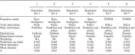
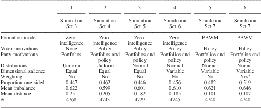
The first column of Table 3 reports the mean scores for all three measures in the simulations. Interestingly, the proportion of one-sided governments (0.447 or 44.7 percent) is very similar to the mean level reported in Table 1, which is based on the same distribution of party system sizes. The mean level of imbalance is 0.622, which corresponds to a government in which 81 percent of the seats represented in the cabinet belong to one side of the first dimension. The final measure, mean distance, has a value of 0.251, indicating that the average government is positioned about half way between center and an end of the first dimension.
The Effect of Moving the Baseline Model Toward Greater Realism
Note: In all simulation sets, systems in which all parties were located on one side of center were excluded.
PAWM=proportional allocation + weighted mean.
a Party systems are weighted runs according to the relative frequency of their effective numbers of parties in Strøm, Müller and Bergman’s (Reference Strøm, Müller and Bergman2003) 17-country data set.
This baseline model thus suggests that GGS’s two rules of parliamentary government do not significantly alter the substantial level of one-sidedness that a random process would produce. But this might be misleading, because the model embeds more than just these rules, plus the assumption that parties are office-seekers. It also assumes a variety of other conditions, many of which are patently unrealistic. These include the following: (1) systems contain two policy dimensions of equal salience; (2) voters and parties are uniformly distributed in these policy spaces; (3) the zero-intelligence model of government formation is a reasonable choice for investigating bilateralism; and (4) the number of parties per system ranges evenly between three and seven. What would happen if these assumptions were made more realistic? Or more generally, how do variations in these features affect the level of non-centrism in government compositions and policy positions?
Moving the Model Toward Greater Realism
Perhaps the most obvious step in making the model more realistic would be to bring policy back into the picture by allowing voters to choose parties according to policy proximity and parties to evaluate government proposals according to a random mix of their portfolio and policy payoffs. This essentially brings us back to the GGS model, although, as noted earlier, both utility functions are made a little more credible by including a random error component. Column 2 of Table 3 (SS 4) shows the results: there is little change in degree of imbalance or one-sidedness in government compositions, but a more noticeable and statistically significant (p<0.001) decline in distance from the center. The likely explanation is that, with policy relevant for both voters and parties, parties that lie toward the extremes become much less desirable as coalition partners, causing governments positions to move closer to the center, on average. Since the participation prospects of both extreme left and extreme right parties suffer, however, the degree of compositional imbalance is much less affected.
A second questionable assumption is that voter and party positions can be treated as draws from uniform distributions. A better choice would be to use normal distributions, particularly if their parameters vary across systems in ways that are reasonably realistic, as specified earlier (footnote 7). This may not capture every political system on every salient policy dimension, but it is certainly more realistic than assuming across-the-board that the policy extremes are as well-populated as the central area. Re-running the simulations with this one specification change produces the results shown in the third column of Table 3 (SS 5). The consequence is a small but significant (p<0.001) reduction in the mean distance from the center, but virtually no change in the mean level of imbalance.Footnote 8
We should also consider the issue of dimensional saliences. The GGS model and our baseline model assume two dimensions of equal salience, but this is clearly a simplification. In the absence of good empirical information on how these saliences vary in the real world, SS 6 draws the dimensional salience parameter for each run from a uniform distribution that ranges from “0” (only the first dimension matters) to “1” (only the second dimension matters).Footnote 9 Does this make any difference to our indicators of imbalance and distance, which are both calculated from the first dimension only? The results reported in column 4 show only small changes in our indicators, none of which is significant at the 0.05 level. Further research shows that focusing the analysis only on systems where the first dimension is more important than the second does not change the overall tenor of this conclusion.
Another area where realism can be enhanced concerns the model of government formation. SSs 3–6 use the zero-intelligence specification, but we have seen that a PAWM specification, by embedding strong empirical tendencies (proportional portfolio allocations and policy influence), does a much better job of generating governments that reflect vote choices realistically. Does it also affect the level of non-centrism? The results shown in the fifth column (SS 7) suggest that it does, at least in part. While there is relatively little change in the level of imbalance or one-sidedness, there is a pronounced and significant (p<0.001) decrease in mean distance from the center. The average government remains about 80 percent composed of one side of the spectrum, but it adopts a position that is not particularly far from the center, traits that might together be described as “moderate bilateralist.”
Finally, the levels of mean imbalance and mean distance reported thus far assume a political universe in which three-party, four-party, five-party, six-party, and seven-party systems are equally present. While systems with eight or more relevant parties may be uncommon in the real world, it is much less likely that the remaining systems are so equally distributed. In their simulations, Golder, Golder and Siegel (Reference Golder, Golder and Siegel2012, 435) handled this issue by weighting runs according to the relative frequency of their effective numbers of parties in Strøm, Müller and Bergman’s (Reference Strøm, Müller and Bergman2003) 17-country data set. Applying that scheme here produces the results shown in the final column of Table 3. These results reveal relatively little change from the previous column: mean imbalance and distance increase, but only very moderately.
The overall impression that emerges from this section is that developing an increasingly realistic model of elections and government formation tends to result in governments that are closer to the center in policy position but still quite unbalanced in composition. In fact, the levels of one-sidedness reported in Table 3 remain quite similar to the mean rate reported in Table 1, which is calculated on the assumption that government formation is totally unstructured and random. Does this mean that—at least as far as government composition is concerned—we have somehow hit upon a natural level that is essentially immune to structure and motivation?
Despite the similarity in levels of one-sidedness, there are a couple of good reasons to continue to resist this conclusion. The first is that real-world rates of one-sidedness are almost certainly higher than the levels shown in Table 3. As noted earlier, the CPDS data produce a rate of 0.63 or 63 percent and, due to the way the data are coded, this is almost certainly an under-estimate. The CSES data, which do not suffer from this problem, reveal a rate of 0.75 across 88 governments (Warwick Reference Warwick and Druckman2016). The second reason to resist the conclusion is that we have yet to take into account certain factors—specifically valence and compensationalism—that may affect voting behavior in ways that are potentially conducive to bilateralism. We turn to these types of influence in the next subsection.
Adding Complexity to Voter Preferences
To this point, the assumption has been that the only systematic influence on vote choices is policy proximity. This is a very narrow view of what drives these choices. It is well known that certain non-policy or “valence” factors, such as candidate appeal and assessments of party competence, can matter a great deal as well.Footnote 10 There is also evidence that voters may vote compensationally, that is, with a focus on expected government policy, at least to some extent (Kedar Reference Kedar2009). In this section, we look at the impact of both considerations, beginning with the former.
As noted earlier, valence is generally taken nowadays to be an attribute of parties (or candidates), that is, each party’s valence assessment is common to voters, or at least not related to its policy position. To capture this understanding of valence, valence scores for parties in each system were drawn from a continuous uniform distribution with range [0, 1] and converted into proportions. These proportions were then rescaled so that the average valence per system is equal to the average voter-party distance (see Online Appendix for details); this allows a mixing parameter, β val, to be used to determine the weight or salience of the valence component relative to the distance component in the voter utility function for each system. In the simulations reported here, β val is also drawn from a uniform distribution with range [0, 1], so that systems vary uniformly from those in which voters care only about proximity to those in which voters care only about valence.
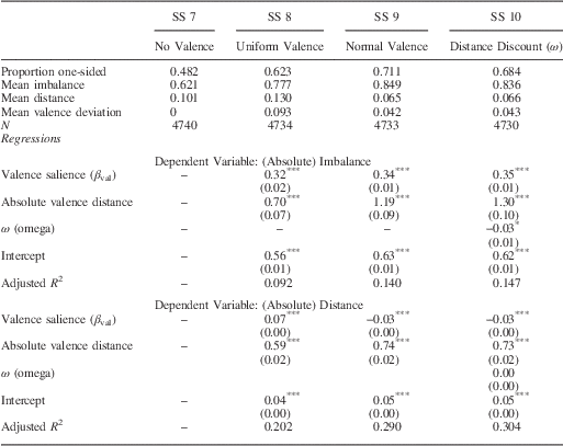
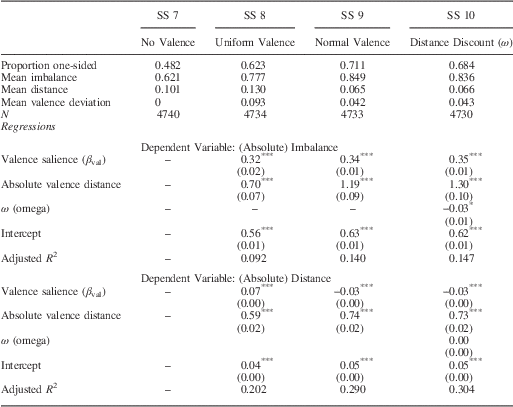
The effects of introducing valence on the aggregate measures of non-centrism are shown in Table 4. The top portion of the table reports the aggregate levels. The first column repeats the levels from column 5 of Table 3 to provide a baseline for these comparisons. The second column presents the levels for SS 8, in which valence, as defined above, has been added to voters’ utility calculations (with all other assumptions remaining the same). The overall effect of this change is clearly to make governments much more imbalanced in composition and non-centrist in policy positions (all differences are significant at p<0.001). But how much valence has been introduced to generate these increases? One way to assess this would be to calculate the mean valence distance, that is, the (absolute) distance between the valence-weighted mean party position on the first dimension and the center of the dimension, averaged across runs. In the parliamentary elections of the CSES (2003–2013) for which reliable data are available, the mean valence deviation is 0.050 units on our 0–1 scale.Footnote 11 The corresponding figure for SS 8 is 0.093, suggesting that the valence introduced in these simulations is excessively lopsided.
Valence Effects on Bilateralism
Note: In simulation set (SS) 8, raw valence scores are drawn from uniform distribution (0, 1); for SS 9 and SS 10, they are drawn from N (0, 0.1).
In the regressions, standard errors are given in brackets.
*p<0.10, **p<0.05, ***p<0.01.
The problem may be that allowing any party, regardless of how small or extreme, to receive a high valence rating is unrealistic: the larger, more central parties may be much more likely to benefit from valence effects. This suggests the following strategy: imposing a normal distribution onto the first dimension of each system and allocating each party in the system a valence score corresponding to the height of the curve above its position (then rescaling these scores as before). With respect to the parameterization of this distribution, I was again guided by the CSES (2003–2013) data, whose average standard deviation in party valence is equivalent to about 0.1 on the 0–1 scale used here, with a SD of about 0.03. Using these specifications, the results shown in the third column of Table 4 were produced (SS 9). They reveal a much lower level of valence distance: just 0.042 on average, which is even less than in the CSES data. This results in a considerable lowering in the mean policy distance of governments, but also a substantial increase in the mean levels of one-sidedness and imbalance. The reason for both outcomes is that valence is now favoring larger, more centrally located parties, putting them in a stronger position to form governments by themselves or with close neighbors and to impose their own policy preferences. In fact, so strong is this effect that both mean imbalance and the rate of one-sidedness now approximate their equivalents in the CSES data (0.813 and 0.746, respectively).
This similarity with real-world levels of imbalance and one-sidedness should not be taken to imply that we have now accurately reproduced the real world; after all, it is highly unlikely that the salience of valence in voter utility calculations varies uniformly from 0 to 100 percent across systems in the real world, as in these simulations. What is more important is that the simulations demonstrate how strongly governmental imbalance and distance may respond to valence influences. These effects are further explored in the regressions reported in the lower portion of the table, which show the impact of the valence salience parameter and the valence deviation on the two measures of bilateralism.
In both the SS 8 and SS 9 simulations, the regressions reveal that the salience of valence in an election and its mean distance from the center produce significantly higher levels of imbalance in government composition. These factors also significantly increase the distance of the government’s policy stance from the center in SS 8, but not in SS 9. In the latter, the concentration of valence in the center of the policy space means that as valence becomes more important, governments move significantly closer to the center. This is consistent with the mean levels of distance shown in the upper portion of the table. It is noteworthy, however, that even here the valence distance is by far the dominant influence on government positioning.
The results presented thus far are based on the idea that valence is a perception of competence or appeal that is common to all voters. Recent research has suggested, however, that the valence rating a voter gives a party, all else equal, may decline according to the policy distance between their positions (Zakharova and Warwick Reference Zakharova and Warwick2014). This conception of valence is captured in the simulation program by means of another mixing parameter, ω (omega), that discounts valence in voter utility functions according to policy distance (see Online Appendix for details).Footnote 12 To assess the impact of this conception of valence, another set of simulations (SS 10) was produced, identical to SS 9 except that valence is discounted by voter-party distance. The ω parameter that determines the rate of discounting in each system was randomly drawn from a uniform distribution with range [0, 1]. The results are shown in column 4 of the table.
Given that the valence effect is being discounted by policy distance, one would expect the mean levels of imbalance and distance to decline somewhat from SS 9. This turns out to be true only for mean imbalance, however, and the degree of decline is not especially impressive (given that these simulations allow the distance discount to become quite large). This is confirmed in the regression analyses, where the effect of the ω parameter on imbalance is relatively small and just barely significant at the 0.05 level (p=0.023). Apparently, valence stimulates the emergence of moderate bilateralism even when it is discounted to some extent by policy distance.
Let us turn now to the other more complex characterization of voter behavior, compensationalism (Kedar Reference Kedar2009). The idea here is that voters vote for the party that will do the most to move expected government policy closer to their own positions on the first dimension. As noted earlier, the simulation program implements the version in which expected government policy is estimated by the seat-weighted mean position of all legislative parties. Since this mean generally falls close to the middle of the dimension, the overall result of compensational thinking is to cause voters to support parties that occupy more extreme positions on their side of center. In terms of bilateralism, the expectation is that this tendency to support non-centrist parties will pull government policy and composition away from the center.
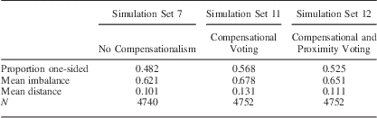
The effects of compensationalism are reported in Table 5. For purposes of comparison, the first model repeats the results from SS 7, which had neither valence nor compensational effects. In the simulations reported in the second column (SS 11), all specifications are the same except that voting follows the compensational logic. The result is a strengthening of bilateral effects: governments are less balanced on average and their policy positions tend to be further from the center. All differences are statistically significant (p<0.001).
Compensational Effects on Bilateralism
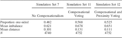
Note: In all simulation sets, systems in which all parties were located on one side of center were excluded.
Because we cannot be sure that all voters use a compensational logic, Kedar estimated models in which voter utility functions are weighted combinations of compensational and proximity components. In the simulations program used here, the mixing parameter θ (theta) determines the relative extent to which proximity prevails in individual voting decisions in a given system. Allowing θ to vary randomly across the range [0, 1] produces the aggregate levels shown in the third column of the table (SS 12). Clearly, the impact of bringing some degree of proximity voting back into the picture is to reduce the propensity for governments to be imbalanced in composition and non-centrist in policy stance, on average. As one might expect, these reductions are approximately proportional to the relative decline in the importance of compensational voting.
All in all, the simulations reported here show that valence and compensational voting both have the potential to affect the extent to which government compositions and policy stances favor a single side of the left-right spectrum. Certain compromises with reality have had to be made in generating these results, to be sure. It was assumed, for example, that all voters in a given system attribute the same importance to valence assessments, whereas in reality this will vary within as well as across systems. Similarly, it was assumed here (and in Kedar’s work) that voters mix proximity and compensational considerations according to a shared weighting, although a more likely scenario is that some voters use a compensational logic while others do not, or at least that if they combine the logics, they vary in the relative weight they give to each. Nonetheless, it seems unlikely that these compromises invalidate the conclusions that bilateralism will be enhanced to the extent that voters act upon valence assessments that disproportionately favor one side of the left-right spectrum or employ a compensational logic that encourages voting for relatively more extreme parties.
DISCUSSION AND IMPLICATIONS
The purpose of this series of simulation experiments has been to identify factors that may lie behind the tendency for parliamentary governments to be composed primarily from one side of the left-right spectrum and to adopt non-centrist policy positions. Because many factors may combine to translate voter preferences into governmental outcomes in ways that are, as yet, incompletely understood, and because some of these factors lack real-world variability or measurability, the approach adopted here has been to explore their roles through simulation experiments. Wherever possible, the simulations have specified parameters that resemble their real-world equivalents or at least that vary in ways that allowed their potential effects to be assessed. What, precisely, have we learned?
The inquiry began with the recognition that a purely random process of government formation will generate a certain level of compositional one-sidedness whenever a center exists. This level increases only moderately when the government formation process is constrained to accord with the two basic rules of parliamentary government. Applying these rules entails other assumptions, but it is important to remember that levels of one-sidedness or imbalance remain reasonably invariant to many of them. In other words, there is an intrinsic one-sidedness to the entire election and government formation process that is relatively unaffected by the distribution of voters and parties, the goals they seek, the constraints on how coalitions are put together, and so forth. Where these factors do have a very perceptible effect is in terms of the government’s policy position relative to the center. A focus on minimizing policy distance, together with more center-concentrated voters and parties, are clearly associated with the emergence of less extreme government positions, on average.
These results might suggest a picture in which government policy tends toward the center and compositional imbalance is limited at most, an interpretation that might be seen as reasonably consistent with the idea of congruence. What can clearly upset this picture, however, is any sizeable tendency for voters to be guided by valence assessments that favor one side of the left-right spectrum over the other. This might happen if a certain party leader happens to be particularly popular, for example, or more simply if an incumbent government or leader has become particularly unpopular. As valence becomes more important to voters, the party or parties favored by these considerations become increasingly able to form governments by themselves or in conjunction with near-by allies, which enhances one-sidedness or imbalance in government formation. Whether it enhances policy non-centrism depends on where the favored parties are located on the left-right dimension: if they are relatively distant from the center, it might increase it as well.
Another factor that is likely to make a difference is compensational voting. In the simulations, it increases both one-sidedness in government composition and policy non-centrism. The motor for both effects is the tendency of compensational thinking to encourage voters to choose parties that are more extreme, policy-wise, than they are. For this reason, it seems probable that any other type of strategic thinking that carries this implication—such as directional voting (Rabinowitz and Macdonald Reference Rabinowitz and Macdonald1989), to cite one prominent example—will also enhance bilateralism.
These findings are all hypothetical, of course: they are based on simulations that incorporate simplifications and assumptions that seem plausible but may nevertheless be wrong. The advantage of undertaking them is that they point us in directions where empirical evidence should be sought. For instance, we know very little about how valence manifests itself in actual electorates—how it is distributed, how much weight voters give it, and so forth. The same holds for the extent of compensational voting. The experimental evidence reported here suggests that they should be pursued more thoroughly, since their impact may extend beyond individual vote choices to encompass the basic structure of party competition and government formation as well.
Speaking of basic structures brings to mind the instrument through which these findings and implications have been reached. That instrument is the Elections and Governments Program, which enormously expands GGS’s zero-intelligence software. Although it was created to explore the sources of one specific phenomenon, its capabilities in simulating elections and government formation under a wide variety of conditions (well beyond those used here) are quite general. If the premise is granted that it has proved useful in investigating bilateralism, it seems reasonable to expect that it could also prove valuable in investigating other major aspects of democratic governance.
ACKNOWLEDGMENTS
This research was funded by the Social Sciences and Humanities Research Council of Canada (Grant 435-2013-0255). The Elections and Governments program was coded by Irina Zakharova with the assistance of Maria Zakharova. I want to thank all concerned for their contributions.