

In his Wealth of Nations, Adam Smith remarked that ‘the discovery of America, and that of a passage to the East Indies by the Cape of Good Hope, are the two greatest and most important events recorded in the history of mankind’ (Smith Reference Smith and Cannon1776, IV.7.166). For Europe, the benefits of the new trade routes were clear and numerous (Findlay and O'Rourke Reference Findlay and O'Rourke2007; Acemoglu, Johnson and Robinson Reference Acemoglu, Johnson and Robinson2005). In contrast, the experience of the territories outside Europe was ambiguous (O'Brien Reference O'Brien1982). Within this context, it is particularly important to study the role of the Cape trade route in the early economic development of South Africa, given that the Cape Colony was the halfway route to the East.
Volumes have been written on the impact of the Cape route on trade between Europe and the East (De Vries Reference de Vries, Flynn, Giráldez and Von Glahn2003; Prakash Reference Prakash2004; Shiue and Keller Reference Shiue and Keller2007), but there is as yet little understanding of the economic impact of the trade route on the development of markets in Southern Africa (apart from the larger literature of colonisation and African underdevelopment; see, for example, Bertocchi and Canova Reference Bertocchi and Canova2002). Different to other territories, the Cape of Good Hope was not considered an important trade destination in itself; the settlement was founded in 1652 by the Dutch East India Company (Vereenigde Oostindische Compagnie, or VOC) with the sole purpose of providing passing Dutch ships with fresh water, food and fuel (Ward Reference Ward, Bentley, Wigen and Bridenthal2007). The historical literature suggests that the Cape exported relatively few goods to European markets (apart from small quantities of ivory and aloe amongst others); most of its exports of wine, brandy and wheat were of poor quality and sent to markets in the East (de Kock Reference de Kock1924; Ross Reference Ross, Elphick and Giliomee1990).
Economic historians traditionally regard the Cape Colony of the seventeenth and eighteenth centuries as an impoverished and destitute settlement (de Kock Reference de Kock1924; Schutte Reference Schutte, Elphick and Giliomee1980; Giliomee Reference Giliomee2003; Feinstein Reference Feinstein2005). To some extent, the slow progress could be ascribed to the mercantilist policies promulgated by the VOC at the Cape; farmers were only allowed to sell their produce to the VOC at predetermined prices, free trade with passing ships was disallowed, heavy import and export duties were levied and manufacturing was prohibited within the colony (Feinstein Reference Feinstein2005). It was thought that ship traffic was the main contributor to economic growth and development in the colony, and with the stagnation in the number of ship arrivals throughout much of the eighteenth century, the economy stagnated too.
However, van Duin and Ross (Reference van Duin and Ross1987) and, more recently, Brunt (Reference Brunt2007), challenged the view of the Cape as a poor-performing economy reliant on external demand. Using the opgaaf rolls (tax return records) obtained from Dutch archives, these authors argue that the early Cape economy was a competitive market economy, exhibiting strong growth throughout the eighteenth century. In contrast to the traditional argument that passing ships – with no increase in numbers for most of the eighteenth century – were essential to the welfare of the Cape Colony, van Duin and Ross (Reference van Duin and Ross1987, p. 8) emphasise the dominant role of local demand, which is demand for consumption within the Cape Colony beyond exports and ship provisions, i.e. demand not directly related to ship traffic.
Yet, there are a number of reasons why ship traffic would have been important to a dynamic Cape economy. Three important demand-generating impacts can be identified. First, ships visited Cape Town to acquire local resources for their journey ahead, notably food, fuel and water. Second, some goods, especially wheat, wine and brandy, were exported and, therefore, carried by ships. Because of the prohibitions on industrial activity, nearly all manufactures were also imported. Third, the Cape provided services to the roughly 10,000 soldiers and sailors visiting the colony each year. In fact, the Cape offered health and travel services on a massive scale; as one historian put it: ‘According to seamen, nearly every house in Cape Town was a public house or inn’ (Schutte Reference Schutte, Elphick and Giliomee1980).
The article tests the hypothesis that economic activity, as reflected in agricultural production, was systematically related to the demand from passing ships. A systematic analysis requires quantitative data and the article uses a time-series smoothing technique borrowed from the business cycle literature to extract useful information from the noisy historical time series. Econometric tests for long-run relationships are applied to the smoothed data to test the hypothesis, with results disaggregated by type of agricultural good. The economic sizes of these relationships are also briefly evaluated.
The article first presents a review of the literature on early Cape economic activity in relation to ship traffic and identifies the hypotheses to be tested. Thereafter, the article discusses the econometric methodology and the time series data and explains how time-series smoothing can assist in extracting useful information from these data. The article ends with a discussion of the results and the conclusion.
1. Economic activity in the early Cape Colony in relation to ship traffic
The first Europeans to settle in South Africa arrived in 1652 to establish a halfway station for VOC ships sailing between Europe and the East Indies. The establishment of the halfway station represented a pre-emptive move to capture a strategic location for the Netherlands (Schoeman Reference Schoeman1999). The VOC did not intend initially to develop the Cape station into a colony for European settlement. Rather, the first Dutch commander, Van Riebeeck, envisaged a European blueprint of farms nestled around the Fort, providing fresh produce to passing ships. Cattle and other commodities were to be bartered from the indigenous Khoikhoi pastoralists. Growing demand from ships and an unwillingness by the Khoikhoi to sell their most valuable commodity soon resulted in European raids and, with European advantages in weaponry and disease (such as the smallpox epidemic of 1713), a loss of territory that accelerated the expansion of the colony. The VOC facilitated this process of expansion, with land grants to contract-expired soldiers, sailors and other servants of the VOC. Nevertheless, European immigration was discouraged, forcing nearly all farmers, including those on the frontier, to find alternative forms of labour, both for agricultural production and within the household. Slave and indentured labour, imported from Madagascar (66 per cent), Mozambique, India and the East Indian archipelago, as well as coerced Khoikhoi, would become the dominant source of labour for the Company and colonists (Armstrong and Worden Reference Armstrong, Worden, Elphick and Giliomee1990; Ross Reference Ross1983a; Worden Reference Worden1985; Shell Reference Shell1994; Newton-King Reference Newton-King1999; Fourie and Von Fintel forthcoming). The slave population exceeded the European population at the Cape throughout the eighteenth century.
By the turn of the century, the area west of the first mountain ranges had been settled. Production appears to have met local demand, especially after more land had been awarded to the French Huguenots of 1688 (Fairbridge Reference Fairbridge1931; Guelke Reference Guelke, Elphick and Giliomee1980). Farmers now moved into the area beyond the first mountains, turning to pastoral, cattle farming (Van der Merwe 1936). There is some evidence to suggest that these farmers were relatively poor, and remained so throughout the eighteenth century, while a small elite developed in the wheat and wine area west of the mountains and closer to Cape Town (Ross Reference Ross1983b; Dooling Reference Dooling2005; Fourie and Von Fintel Reference Fourie and Von Fintel2010). Three distinct groups could therefore be identified: the group of VOC officials, traders and artisans in and around the fort; the wine and wheat farmers; and the pastoral farmers of the interior, with diminishing contact with the market the further they moved from the fort.Footnote 1
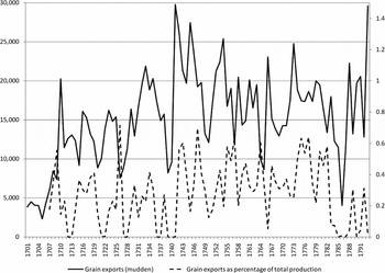
Agricultural production was limited to a few commodities: wheat, barley, rye, grapes, cattle, sheep, pigs and horses, of which wheat, grapes (wine) and cattle were the most prominent (Guelke Reference Guelke, Elphick and Giliomee1980; Feinstein Reference Feinstein2005).Footnote 2 While wine exports were relatively small and of poor quality, grain exports grew significantly during the eighteenth century, notably wheat exported to the Dutch settlements in the East. Figure 1 reports total grain exports (in muddenFootnote 3) and grain exports as a percentage of production (which has been adjusted using the van Duin and Ross (Reference van Duin and Ross1987) coefficients, reported on the secondary axis). Nearly 40 per cent of all grain produced between 1740 and 1780 was exported to the colonies and the Netherlands. Apart from the fresh meat consumed by sailors on their voyages, other exports were relatively insignificant, and included peas and beans, butter, fat, meat, bacon, tallow, aloe, ivory, wax and train oil. This is in sharp contrast to the view of earlier economic historians who suggested that: ‘At the Cape . . . trade was subject to numerous restrictions, and even prohibitions, as a result of which there was hardly any outlet for the surplus produce of the colonists. There was virtually no foreign trade and very little internal trade, and consequently the Cape advanced with almost extreme slowness’ (de Kock Reference de Kock1924, pp. 39–40).
Grain exports, 1701–93

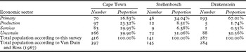
Agricultural production by no means constituted the whole of the Cape's economic activities. As the only port and physical market of the Cape Colony, Cape Town housed a variety of tertiary sector activities (Worden, van Heyningen and Bickford-Smith Reference Worden, van Heyningen and Bickford-Smith1998). Table 1 presents a survey conducted in 1732 by then Cape Governor Jan de la Fontaine, revealing the relative distribution of occupations for free burghers over the three districts of the colony. In the final row, the total number of survey candidates is compared to the total population as suggested by an alternative source. This indicates that the survey, in fact, covered the entire population (or, at least, the total number of white and free black people in the Cape Colony).
Survey of occupations in Cape Colony, 1732

Source: Schutte (Reference Schutte, Elphick and Giliomee1980, p. 189).
Table 1 suggests that at least 40 per cent (and probably much more) of those living in the district of Cape Town were involved in secondary and tertiary activities. Furthermore, the survey excludes VOC officials, who totalled 1,016 at the time – many of whom were involved in services occupations in Cape Town or were part of the private and illegal trade.
The relationship between ship traffic and tertiary sector activity receives attention from van Duin and Ross as well as in some other works. Van Duin and Ross (Reference van Duin and Ross1987) agree that ‘the money the ships and their crews brought into Cape Town, and spent on lodging, food, drink and the minor trade . . . may indeed have contributed, through the multiplier effect, to the prosperity of [the] colony in ways we have been unable to measure’. In fact, historians suggest that Cape Town was known as the ‘Tavern of the Seas’, and offered many public houses and inns to weary travellers (Giliomee Reference Giliomee2003, p. 28; Schutte Reference Schutte, Elphick and Giliomee1980, p. 189). Boucher (Reference Boucher1974, p. 20) offers some anecdotal evidence: ‘The settlement offered . . . rest, recovery, good food and entertainment after long months at sea. A typical seaport, it provided pleasures at various levels, from the dubious delights of tavern and brothel to the convivial company of well-to-do burghers and the enjoyment of country excursions.’ These sentiments are reiterated in his descriptions of ships arriving between 1735 and 1755 at the Cape (Boucher Reference Boucher1985).
From 1720 to 1780 an average of between 9,700 and 11,600 men per year left either Europe or Asia on the ships of the VOC. Almost all of these men, except those who had perished on the ships, would have visited Cape Town, spending several weeks recuperating from the long voyage (van Duin and Ross Reference van Duin and Ross1987, p. 13). In modern-day terminology then, the Cape was a hub of travel service exports, i.e. tourism expenditure on accommodation, food and beverages, entertainment and health services (Fourie, forthcoming).Footnote 4 Compared to the 2,063 free burgher population in 1720, which slowly increased to approximately 8,000 in 1770 and 15,000 in 1795 (Beyers Reference Beyers1929), the influx of foreign visitors must have had a sizable impact on the economy of the Cape, at least during the early decades of the eighteenth century (Guelke Reference Guelke, Elphick and Giliomee1980; Sleigh Reference Sleigh1993).Footnote 5
Prices would typically be related to swings in demand and supply and should be closely correlated with demand induced by the passing ships. However, the prices paid by the VOC for farmers’ produce were not determined by a market system at the Cape; the Dutch East India was a monopsonist buyer of agricultural produce, restricting prices at low levels throughout most of its 143-year rule (Ross Reference Ross, Elphick and Giliomee1990). These prices changed only by decree and did not necessarily reflect the market demand or supply for goods and services. As expected, this was an unpopular policy and generated frequent petitions and protest from the farming community, of which the most famous was the Patriot movement towards the end of the eighteenth century (Schutte Reference Schutte, Elphick and Giliomee1980).
Furthermore, the VOC prohibited direct trade between farmers and foreign ships, as well as any industry. Monopoly rights were sold to individuals, mostly in the lucrative industries of beer brewing and bread-baking (Groenewald Reference Groenewald2007). These policies were profitable to the VOC, but detrimental to the economic development of the Cape. While illegal trade did occur (with passing ships and with the local Khoikhoi), there is little evidence that this was, on average, an important part of farmers’ incomes.
The preceding subsections briefly reviewed evidence concerning economic activity in the early Cape Colony. In particular, the work by van Duin and Ross (Reference van Duin and Ross1987) receives significant attention, by virtue of the importance of their research in altering economic historians’ view of the early Cape economy – changing it from a subsistence-based to a market-based view. However, van Duin and Ross emphasise local consumer demand in driving agricultural production growth, although they agree that economic activities in Cape Town may have been more closely related to ship traffic. The secondary position accorded to ship traffic as a source of demand for agricultural produce is in contrast to various historical sources; Boucher (Reference Boucher1974, Reference Boucher1985) and, more recently, Ward (Reference Ward, Bentley, Wigen and Bridenthal2007, Reference Ward2008) document the role of maritime traffic in Cape social life. The literature therefore suggests that ships arriving in Table Bay had three important demand-generating impacts.
First, the ships required the replenishment of food, water and fuel supplies for the journey ahead (for example, see Appel Reference Appel1966 and Roux Reference Roux1975 on the demand for wood as fuel and for ship repair and maintenance). This was the original purpose of the halfway station at the Cape and perceived to be the main economic benefit, also by Adam Smith:
The Cape of Good Hope . . . is the half-way house, if one may say so, between Europe and the East Indies, at which almost every European ship makes some stay, both in going and returning. The supplying of those ships with every sort of fresh provision, with fruit and sometimes with wine, affords alone a very extensive market for the surplus produce of the colonists. (Smith Reference Smith and Cannon1776, Book IV.7.186)
Second, and especially after production in the local economy had increased to above subsistence levels, some products were bought for export, especially wheat, wine and brandy destined for the East Indies. In addition, most manufactured items had to be imported from Europe.
Third, Cape Town offered crews arriving on ships after several months at sea the opportunity to heal and rest. In fact, the demand from the VOC hospital, inns, pubs, and other institutions with strong links to ship traffic would have represented a significant share of the local demand defined by Van Duin and Ross (Reference van Duin and Ross1987). A systematic relationship between ship traffic and agricultural production beyond exports may therefore suggest that travel services exports constituted an important economic activity in the Cape Colony.
The three demand-generating impacts suggest the following hypothesis for this study: economic activity in the Cape Colony of the eighteenth century was systematically related to ship traffic in Cape Town harbour. Given the earlier discussion on price stability, economic activity is measured in terms of the quantity of wheat, wine and cattle production. Non-rejection of the hypothesis would suggest a significant role for ships in the Cape economy.
2. Methodology
Van Duin and Ross (Reference van Duin and Ross1987) rely on a predominantly descriptive analysis to study the relationship between ship traffic and Cape economic activity: they use graphs and qualitative data description to compare five-year averages for ship traffic and agricultural production. This article employs econometric analysis of annual data to reconsider the relationship. As described below, econometric analysis enables a systematic study by focusing on an average relationship over time, while allowing for noise due to relationships with other variables.
Pesaran, Shin and Smith (Reference Pesaran, Shin and Smith2006) suggest an econometric method to test for the existence of long-run relationships based on the first step of the autoregressive distributed lag (ARDL) approach to co-integration. The advantage of their method over conventional co-integration tests (such as the Johansen Reference Johansen1988 system approach) is that it overcomes the need for unit root pre-testing – i.e. it is not necessary to know whether the time series contain stochastic trends in order to apply the technique. The method is based on the following ARDL(p) model:


where y is a measure of economic activity (such as wheat production), x is a measure of ship traffic and p is the lag length (in years). All variables are in logarithmic form.
The method consists of testing the null hypotheses β1=β2=0 and β3=β4=0 against two-sided alternatives. The null hypotheses β1=β2=0 and β3=β4=0 serve to establish, firstly, whether a long-run co-integration relationship exists between yt and xt and, secondly, whether one of the two variables is long-run forcing (i.e. whether the long-run relationship is unidirectional). The intuition of the method lies in its close analogy with tests of weak exogeneity in co-integrated systems (Ericsson and Irons Reference Ericsson and Irons1994; Engle, Hendry and Richard Reference Engle, Hendry and Richard1983): the equations above can be seen as representing a co-integrated system, with the β coefficients representing the long-run adjustment parameters. For example, if the hypothesis β1=β2=0 is rejected, this is akin to suggesting that the variable yt is weakly exogenous and does not contribute towards re-establishing a long-run equilibrium between yt and xt.
Null hypotheses of the form β1=β2=0 and β3=β4=0 involve multiple parameter restrictions and are usually tested using an F-statistic, which is compared with some critical value at a prescribed significance level. Pesaran, Shin and Smith (Reference Pesaran, Shin and Smith2006) suggest a bounds-testing approach, which involves two critical values (an upper and a lower bound) depending on the time series properties of y and x. Values falling below the lower bound indicate the absence of a systematic relationship, while values exceeding the upper bound confirm such a relationship. Where the test statistics fall between the two critical values, it is necessary to test for unit roots in the individual series. If both series contain unit roots, the upper bound is the critical value. Where both series are stationary, the lower bound is the critical value. In cases where one variable is stationary and another contains a unit root the test is inconclusive if the test statistic falls between the boundary values.
If (equations 1) and/or (2) suggest the existence of long-run relationships, one may use the estimated coefficients in these equations to estimate long-run relationships:


where π0=−α0/β1 and π1=β2/β1 and, similarly, λ0=−φ0/β3 and λ1=β4/β3 and νt are zero-mean stationary (Atkins and Coe Reference Atkins and Coe2002).
3. Data
The econometric methodology described above requires consistent time series data on various forms of economic activity as well as on ship traffic. The following subsections describe the agricultural production data for wheat, wine and cattle as well as the ship traffic data used in this study.
3.1. Wheat production
Traditionally, literature on the economic history of the Cape Colony holds that wheat production did not increase significantly during the eighteenth century. De Kock argues that restrictions on trade with passing ships and, more generally, on exports from the Cape Colony frequently generated cereal shortages:
This continued throughout the eighteenth century and led to a repetition of famines in bad years. Many farmers, having found by experience that they could not dispose of their surplus produce at satisfactory prices or even at all, adopted the custom of sowing only sufficient grain to meet the needs of their own family. If the crops turned out to be a failure in some districts on account of unfavourable weather conditions, a deficiency in the supply of grain might easily result, as such farmers had not allowed for a surplus. (Reference de Kock1924, p. 48)
De Kock offers only anecdotal evidence, citing a shortage in 1786 and a report from De Mist in 1792, stating that the Cape had only eighteen days’ supply of cereals and attributing this to the ‘ill-conceived intentions and bad statesmanship of the Directors of the Dutch East India Company’ (de Kock Reference de Kock1924, p. 48). These have led economic historians to argue that the supply of wheat in the Cape Colony only levelled with demand by the turn of the eighteenth century.
Van Duin and Ross (Reference van Duin and Ross1987) challenge the view of persistent wheat shortages and argue that the official opgaaf data on which historians rely is inaccurate and that production growth was much higher. The opgaafrollen were the rolls on which the annual returns of population and production were recorded by the VOC. Given that opgaaf records were the basis on which taxes on grains were calculated, van Duin and Ross argue that there was an incentive to under-report grain production levels and that the level of under-reporting was significant: Van Duin and Ross (Reference van Duin and Ross1987) note, for example, the bizarre situation of grain exports exceeding official production figures for the period 1769–83. These authors then use corrective coefficients to adjust the official opgaaf figures and also to test the plausibility of the adjustment via a comparison with other relevant information. The corrective coefficients are based on the demand for wheat in the Cape, which is the total of local consumption, consumption by ships and their crew, and exports. A comprehensive explanation of the size and construction of the corrective coefficients is provided in van Duin and Ross (Reference van Duin and Ross1987, pp. 21–31).
Until recently the corrections have not been discussed, though Armstrong (Reference Armstrong1988) notes that the correction coefficients appear to be plausible: ‘[H]igher figures will merely strengthen the . . . thesis, while lower figures seem unlikely.’ However, Brunt (Reference Brunt2007) has recently revised the van Duin and Ross corrective coefficients further upward. While van Duin and Ross (Reference van Duin and Ross1987) are successful in better accounting for year-to-year changes in the opgaaf data, Brunt (Reference Brunt2007) argues that they under-estimate the overall trend in wheat output. Assuming that wheat output and consumption should be equal on average, Brunt (Reference Brunt2007) uses, first, a wheat consumption model to estimate the trend in wheat output and, second, other cross-validation techniques to estimate wheat output at the start and the end of the time series (see appendix 2 in Brunt (Reference Brunt2007) for a complete discussion).
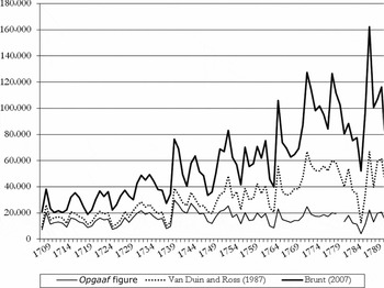
Figure 2 reports the estimates of wheat production by Brunt (Reference Brunt2007) and van Duin and Ross (Reference van Duin and Ross1987), showing that the corrections significantly alter the general pattern suggested by the original opgaaf series. Note that Brunt (Reference Brunt2007) also adds estimates of ‘bread corn’ (in other words, on-farm wheat consumption). Bread corn estimates may also be added to the original opgaaf figures and the van Duin and Ross (Reference van Duin and Ross1987) estimates. We do not attempt this, as we do not have access to these estimates, but see Figure A2 in Brunt (Reference Brunt2007).
Wheat production estimates, 1709–93

The quantitative evidence suggests that wheat production did not increase significantly during the first two decades of the eighteenth century, although the level of output is certainly higher than initially estimated. This is consistent with other historical accounts that report a number of poor harvests, especially in the Stellenbosch district, over this period (Sleigh Reference Sleigh1993, p. 15). However, the second half of the 1720s and the early 1730s saw a rapid increase in production. The 1740s was a period of dissatisfaction, according to van Duin and Ross (Reference van Duin and Ross1987, p. 30). Between 1743 and 1745, following a reduction in the official price of wheat, there were numerous complaints from farmers about their precarious financial position. Travellers in the interior of the country note that many of these farmers lived in poverty and complained of the unstable demand for their produce (Thunberg Reference Thunberg1986, p. 94). The farmers requested a revision of the price, a reduction in taxes and free trade of their goods (van Duin and Ross Reference van Duin and Ross1987, p. 30). Yet, by the end of the 1740s, even though the VOC did not respond to these requests, wheat production had picked up again, showing rapid growth until the early 1750s. Until the mid 1760s, wheat production fluctuated, with serious harvest failures in the Cape district in 1764–5. Wheat production then increased at a dramatic pace until the early 1780s, after which it declined sharply. According to van Duin and Ross, harvests were generally poor between 1782 and 1787, with 1786 being particularly disastrous, to the extent that wheat had to be imported from the United States (van Duin and Ross Reference van Duin and Ross1987, p. 31). Thereafter (1789–93), production returned to and exceeded former levels, with 1793 recording the highest volume of wheat production.
In the subsequent econometric analysis, we rely on both the Brunt (Reference Brunt2007) and van Duin and Ross (Reference van Duin and Ross1987) wheat output data to ensure robustness. An alternative to wheat output may be wheat sown, as wheat sown may more readily reflect the production decisions of farmers in response to ship traffic. The problem with wheat sown is that the type of corrections by van Duin and Ross (Reference van Duin and Ross1987) and Brunt (Reference Brunt2007) are not possible. This leads the article to focus on the higher-quality wheat output data, although tests are also run on wheat sown. While it is not identical to wheat sown due to weather conditions and farmer capability, wheat output could not have changed significantly in the medium to long run without concomitant changes in wheat sown.
In addition to overall wheat production data, the article also tests the relationship between wheat exports and ship traffic. As argued earlier, one of the demand-generating impacts of the ships will have been that they carried agricultural exports to the Netherlands and the East. Unlike the other wheat time-series data, wheat exports are surprisingly accurate, mostly due to the monopolist position of the VOC as wheat trader (van Duin and Ross Reference van Duin and Ross1987, p. 17; Brunt Reference Brunt2007). Consequently, this article also tests for a relationship between wheat exports and ship traffic.
3.2. Wine production
Van Riebeeck introduced the first vines in 1655 (van Zyl Reference van Zyl1974) and the first Cape wine was produced before 1659 (de Kock Reference de Kock1924). Viticulture also interested Van Riebeeck's successors. The settlement of Huguenots from France, especially in the district of Drakenstein, gave particular impetus to viticulture, so that winemaking soon became an important branch of Cape agriculture. According to official statistics, the colonists and officials had planted 400,000 vines by 1688 (de Kock Reference de Kock1924, p. 50).
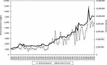
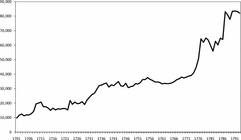
Until 1743, a tax was charged on the basis of the opgaaf records generated from information submitted by farmers. Thereafter, taxes were levied at the moment wine was brought into Cape Town (van Duin and Ross Reference van Duin and Ross1987, p. 43). This measure was an attempt to reduce suspected evasion, as all traffic had to travel along the same road between Devil's Peak and the sea on entry into Cape Town. However, van Duin and Ross argue that, contrary to the data on wheat production, there is no evidence that these figures under-report actual production to a significant extent (van Duin and Ross Reference van Duin and Ross1987). However, they do suggest that the number of vines, rather than actual wine production, may be a more appropriate variable, as the former was probably not as sensitive to bad weather conditions as the latter. Van Duin and Ross (Reference van Duin and Ross1987) provide data for total wine production and the number of vines planted for the period 1700 to 1793 on the basis of opgaaf figures,Footnote 6 as shown in Figure 3.
Wine production and the number of vines, 1701–93

Figure 3 suggests that wine production was generally stagnant for the first four decades, followed by rapid expansion. At first glance, both wine production and the number of vines appear to have a common outlier towards the end of the sample period. Clearly, the value is implausible – especially as far as vines are concerned. However, it can be argued that, although the amplitude is probably overstated, the general upward movement is not. Figure 3 shows long periods of expansion interspersed with short periods of decline, notably in the early 1760s and again in the 1770s and 1780s. According to van Duin and Ross (Reference van Duin and Ross1987, p. 45), these slowdowns were due to harvest failures and not disinvestment. The number of vines also shows no real periods of decline other than during the 1730s.
3.3. Stock farming
With the colony expanding into the interior, cattle farming became more important, as it represented the sole means of subsistence and the only means of transport. The stock farmers of the interior, many of whom lived a nomadic life on the frontier, had little incentive to settle down for long periods of time (Schutte Reference Schutte, Elphick and Giliomee1980). Land was available relatively freely, and as soon as the pasture became depleted the farmers moved on. In this way, the farmers were limited in their accumulation of capital to only those goods that could be transported on ox back or by wagon. Sheep farming was also important, but data problems prevent a further analysis here. Using data from van Duin and Ross, the cattle stock in the Cape Colony between 1700 and 1793 is shown in Figure 4.
Number of cattle, 1701–93
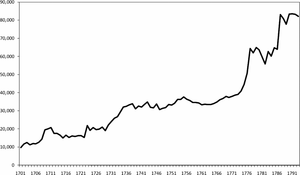
Clearly, there are some problems with the time-series data, similar to the ones mentioned for viticulture (also see Brunt Reference Brunt2007, p 17). For example, the figure above suggests that the number of cattle grew exponentially during the 1770s and again in the late 1780s. These problems will receive attention in a later section.
3.4. Ship traffic data
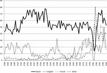
The only reliable estimate of the number of ships that arrived in the Cape Colony was published by Beyers (Reference Beyers1929), who reports the number of ships in Table Bay by nationality, with Dutch, English and French ships representing the dominant share. Figure 5 shows the arrival of ships in Table Bay by nationality between 1700 and 1793. The category ‘Other’ includes ships from Denmark, Portugal, Austria, Prussia, Sweden, Spain, Hamburg, Italy, Russia and America.
Number of ships by nationality, 1700–93

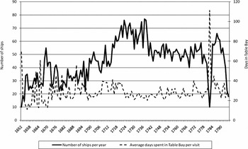
A new electronic data source that includes records of all Dutch ships to anchor in Table Bay since the founding of the VOC has made it possible to extend the period of analysis to 1652 (see Figure 6). The data allow estimates of the number of days ships anchored in Table Bay. Boshoff and Fourie (Reference Boshoff and Fourie2008) have used this to compile a unique data set of ship traffic demand in Table Bay between 1652 and 1793. The original data were compiled by Bruijn, Gaastra and Schöffer (Reference Bruijn, Gaastra and Schöffer1987) in three volumes. The data set requires some cleanup prior to analysis – the final version of the data set is available from the authors on request. A combination of the Bruijn, Gaastra and Schöffer (Reference Bruijn, Gaastra and Schöffer1987) and Beyers (Reference Beyers1929) data sets are used in the econometric analysis of this article.
Number of ships and length of stay, 1652–1795

4. Extracting information from the data
Time-series data of the type discussed above, spanning a century and covering diverse aspects of economic activity, rarely become available to economic historians. Unfortunately, econometric tests using the time-series data may be biased, given that the data are noisy (the wine and cattle-related series in particular), either due to the incentive to under-report or due to the incomplete or inaccurate data collection efforts of the VOC. The challenge, therefore, is to extract the useful information from this data, while minimising the possible loss of information. The work by van Duin and Ross (Reference van Duin and Ross1987) and Brunt (Reference Brunt2007) has contributed significantly to this end, by substantially improving the quality and representativeness of the opgaaf data. However, even these authors advise against using the annual data, given the potential inaccuracy of any given data point. This problem led van Duin and Ross (Reference van Duin and Ross1987, p. 31) to suggest relying on five-year averages, rather than the actual annual figures, when comparing series – given the danger of identifying spurious relationships. The resulting descriptive analysis loses much of the tractability of a systematic time-series evaluation. The next section proposes time-series smoothing methods as an alternative that will reduce the noise created by year-to-year data problems yet retain the explanatory power of the time series.
4.1. Time-series smoothing and its relation to the hypothesis
Economists have developed a range of time-series smoothing techniques to extract specific information from time-series data. Smoothing has been particularly useful in the business cycle literature, where the aim is to separate short-run business cycle information from longer-run trends in the economy (Harding and Pagan Reference Harding and Pagan2002). One popular smoothing technique is the band-pass filter method, which entails decomposing time series into different frequency components where each frequency component relates to a specific time horizon (Baxter and King Reference Baxter and King1999).
The band-pass filter may be useful in solving the data problem in this study: the challenge is to remove information related to short time horizons (as year-to-year movements are quite noisy), while retaining the longer-run information. Apart from removing noise, smoothing out short-term fluctuations also removes the short-run impact on agricultural production of idiosyncratic shocks, such as weather patterns and local strife. While these shocks are important in their own right, the aim of this article is to further explore the market responsiveness of the Cape Colony to ship traffic. This implies a need to focus on long-run relationships based on time series from which shorter-term effects have been removed.
The band-pass filter allows one to refine the analysis even further: in addition to smoothing out short-term noise, the band-pass filter can also remove information related to very long time horizons, leaving a series containing only information related to the medium run. Studying only ‘medium-run fluctuations’ is useful for two reasons.
First, long-term trends in the data may be inaccurate. For wine and, especially, cattle it is particularly difficult to know whether trends are accurate, as the data preclude the type of trend corrections attempted for wheat production (Brunt Reference Brunt2007; van Duin and Ross Reference van Duin and Ross1987). While these data difficulties imply that medium-run fluctuations may also be less accurate, medium-run fluctuations provide signals concerning broad patterns and directions of longer-run movements. More generally, a study of medium-run fluctuations is useful in a pre-industrial setting where there is still disagreement or uncertainty concerning the levels or trends in output, but where it is more generally agreed that output fluctuated over time.
Secondly, and related, medium-run fluctuations are critical to understanding the evolution of longer-run trends. A core insight of the business cycle literature is that long-term trends include medium-run information and are not, as is commonly thought, well represented as straight lines: shorter-run fluctuations carry over into medium-run fluctuations, which, in turn, result in variation in the long-run trend (Comin and Gertler Reference Comin and Gertler2006). If medium-run fluctuations affect long-term trends, a correlation between medium-term fluctuations in ships and output implies a long-run relationship between the trend in ship traffic and the trend in output. A correlation between medium-term fluctuations in ships and output does not merely tell the uninteresting story that trade fluctuations generated output fluctuations; rather, changes in the longer-run trajectory of Cape Town ship traffic over the course of, say, 20 years altered the trajectory of output growth.
‘Fluctuations’ have a connotation of being short-term movements, but in our case we consider both short-run and medium-run fluctuations, the latter being movements around the trend taken over longer time horizons. This is consistent with the use of the concept in the business-cycle literature. The following section discusses the specifics of the band-pass filter, including definitions of the ‘short’, ‘medium’ and ‘long’ run.
4.2. The band-pass filter
As mentioned, the focus on specific frequency ranges requires the decomposition of time series into different frequency bands. Theoretically, such decomposition is possible by virtue of the spectral decomposition theorem (Christiano and Fitzgerald Reference Christiano and Fitzgerald2003). This theorem provides the theoretical basis for the extraction of a specific frequency range via a time series filter called the band-pass filter. The band-pass filter is so named as it ‘passes’ only the specified frequency range – removing other frequency components. The spectral decomposition theorem requires an infinitely long time series. Consequently, in practice, econometricians use approximations to these ‘ideal’ filters. Two approximations have become popular: the Baxter–King (Reference Baxter and King1999) and the Christiano–Fitzgerald (Reference Christiano and Fitzgerald2003) approximations. Zarnowitz and Ozyildirim (Reference Zarnowitz and Ozyildirim2006) note that if the focus is on high-frequency components only, the Baxter–King approximation does not outperform the popular Hodrick–Prescott (Reference Hodrick and Prescott1997) filter (the filter most frequently used in business cycle analysis). However, these authors argue that the Baxter–King filter is useful where the focus is on broader frequency ranges. Everts (Reference Everts2006) argues that the Christiano–Fitzgerald approximation is more suitable for identifying longer-term fluctuations than the Baxter–King approximation. Consequently, this article employs the Christiano–Fitzgerald approximation.
It may be argued that time-series smoothing can be achieved using much simpler methods, such as a moving average filter. The choice of smoothing method is quite important, as it embodies a particular assumption about the role of different frequencies in the smoothing process. Estrella (Reference Estrella2007) notes that time-series filters can either be focused on signal extraction or frequency extraction. Moving averages, for example, are signal extraction filters where a signal can be obtained by calculating an average of a selected number of original series values. Simply taking a moving average of the original series implies that the resultant smoothed series still relies, in part, on the short-run information. This is problematic, given that some individual data points appear to be incorrect. Alternatively, band-pass filters can be used. These are frequency extraction filters where the smoothing is achieved by removing a particular frequency component of the time series. In the case of historic agricultural data, the band-pass filter approach is to be preferred – given that it is likely that the longer-term information is accurate, but that the year-on-year fluctuations are not.
4.3. Smoothing results
The smoothing procedure described in the previous section can now be applied to the original economic and ship traffic series to extract short- and medium-term fluctuations. Before proceeding to the results, however, it is necessary to define the time horizon of short- and medium-term fluctuations to avoid ad hoc concepts. Inevitably, such definitions involve judgment and Burns and Mitchell (Reference Burns and Mitchell1946, p. 469) encountered this challenge during their pioneering business cycle research: ‘Seldom can the interrelated species of social . . . phenomena be marked off from one another with such precision as to leave no doubtful cases.’ Nonetheless, in their study of US business cycles (which can be considered short-term fluctuations) from 1885 to 1931, Burns and Mitchell found cycles to last between one-and-a-half and eight years. Of course, Burns and Mitchell explicitly warned that the range appears to shift over time (Everts Reference Everts2006) – although many contemporary studies of the business cycle continue to employ the one-and-a-half to eight-year range. Consequently, in the context of the present study, it might be useful to consider some comparable figures concerning the South African experience.
Research by Schumann (Reference Schumann1938) on the properties of South African business cycles from 1806 to 1936 offers some guidance concerning the duration of South African business cycles, indicating that business cycle fluctuations lasted between two and twelve years in the period before diamonds were discovered, that is, up to the 1870s. Arguably, the economic fluctuations of this period are closest in nature to those of the eighteenth-century Cape Colony, as the economy was still largely agrarian-based (Schumann Reference Schumann1938, pp. 112–13). On the other hand, there are significant differences between the Cape Colony of the eighteenth and nineteenth centuries, the least of which is not the difference in government. Despite these problems, this article defines short-term (or high-frequency) fluctuations as those cyclical components in the historic time series with a period of between two and twelve years (Comin and Gertler Reference Comin and Gertler2006). Sensitivity tests based on a period of two to eight years do not yield significantly different results.
Medium-term fluctuations can be defined in similar fashion. Unfortunately, less guidance is available concerning the upper bound for the medium-frequency range. This is not necessarily problematic, as Comin and Gertler argue that ‘[e]ven though [their] measure of the cycle includes frequencies up to 50 years . . . its representation in the time domain leads to cycles in the order of a decade’ (Comin and Gertler Reference Comin and Gertler2006, p. 526). These authors argue that this result is an outcome of the spectral density. The frequency definition for medium-term fluctuations appears to be consistent with the findings in Schumann (Reference Schumann1938), who identifies three medium-term cycles in the predominantly agricultural period from 1806 to 1869, with respective duration 30 years, 13 years and 20 years. Again, although these durations are not necessarily comparable to the eighteenth century, they do indicate that the South African economy in its agrarian phase did experience medium-term fluctuations. Equally important, the dubious quality of the time-series data (as discussed above) necessitates a broad view of fluctuations. Therefore, this article defines medium-term (or medium-frequency) fluctuations as those movements in the historic time series lasting between 12 and 40 years (Baxter and King Reference Baxter and King1999). As the upper bound is a subject of debate, sensitivity tests were performed for narrower frequency ranges of 12 to 20 years. Results again do not appear to be significantly different.
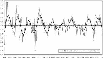
Figure 7 presents short- and medium-term fluctuations for the number of ships in Cape Town harbour.
Short- and medium-term fluctuations in the number of ships, 1652–1793

The line containing circles represents the short- and medium-term fluctuations combined. Put differently, this particular line can be interpreted as the de-trended series, representing the deviations of the actual series from the long-run trend, where long-run is defined as information related to a time horizon beyond 40 years. The solid line represents the medium-term fluctuations (defined previously as that component of the time series with a period of between 12 and 40 years). The short-term fluctuations can be found in the difference between the two lines. Clearly, a substantial amount of short-run noise is present. Lowering the upper bound for the medium frequency from 40 to 20 years does not produce significantly different outcomes.
This smoothing methodology can also be applied to economic time series. As discussed previously, the extracted short- and medium-term fluctuations in the economic and ship traffic data can then be used to test for a relationship. The following section performs the PSS test to study the relationship between ship traffic and economic activity in the early Cape economy.
5. Results
Given the methodology and data adjustment discussed above, we present here the results of the econometric tests of the null hypothesis that ship traffic was systematically related to economic activity in the Cape Colony. The first subsection presents the results based on, first, the unsmoothed time series and secondly, time series smoothed with a moving average filter, to emphasise the importance of the band-pass filter method described above. Subsequently, we present the results based on band-pass filtered data, first removing only short-term fluctuations and then also removing long-term trends.
5.1. Results for agricultural series in unadjusted or moving average form
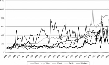
An index of the original ship traffic and the various agricultural time series is shown in Figure 8 (the base value is 100 in 1701). Visual inspection suggests little correlation between any of the economic output variables and ship traffic.
Agricultural production and ship days, 1701–93

These visual impressions are verified econometrically. As discussed in the section on methodology, the analysis is based on the ARDL method developed by Pesaran, Shin and Smith (Reference Pesaran, Shin and Smith2006). For this and subsequent applications of the econometric procedure, a lag of four years is used, as this generally removes serial correlation in the errors. The accompanying 5 per cent critical values for an ARDL with a lag order of four years with an unrestricted intercept and no deterministic trend is [2.86; 4.01] (Pesaran et al. Reference Pesaran, Shin and Smith2006, p. 300).
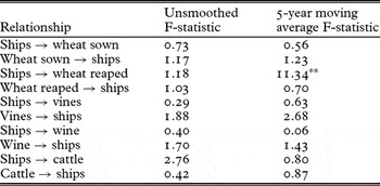
In addition to considering the unsmoothed series, it may also be useful to include smoothed time series using a five-year moving average filter (as opposed to the frequency filters) in the econometric analysis. Table 2 presents the results.
ARDL bounds test results for agricultural production and ship traffic time series

*Statistically significant at 5% **Statistically significant at 1%
As predicted by the visual inspection, Table 2 reports no statistically significant results for the unsmoothed series. Furthermore, the analysis finds no stable long-run relationship between ship traffic and economic activity based on moving average filtered series, except for some evidence of a long-run forcing relationship from ships to wheat production. This is similar to the results of van Duin and Ross (Reference van Duin and Ross1987), employing a moving-average, and concluding that passing ships were only of secondary importance for Cape Colony production. Nevertheless, as argued earlier, the general absence of significant statistical relationships appears to be fundamentally at odds with the qualitative discussion in the historical literature. However, as we have argued above and as the following subsections show, important information is contained in specific frequency ranges of the time series. Focusing on specific frequency components when assessing relationships may, therefore, alter the preliminary findings.
5.2. Results for agricultural time series adjusted for high-frequency fluctuations
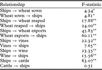
Table 3 reports the results for similar tests on time-series data from which the short-term fluctuations have been removed using the band-pass filter.
ARDL bounds test results for adjusted agricultural production and ship traffic time series (high-frequency fluctuations removed)

*Statistically significant at 5% **Statistically significant at 1%
The results clearly differ from those obtained based on the unsmoothed data set. They suggest that significant long-run relationships exist between ship traffic and all three agricultural time series and that the direction of causality appears to run both ways for wine and wheat production activities. As noted when suggesting the hypothesis, this is not unexpected. If ship traffic represented demand for agricultural produce in the Cape, one would expect economic activity to respond to changes in ship traffic. In some ways, this direction of causality appears to be particularly strong, given the relative size of the test statistics for this direction. However, it may also be argued that increased availability of local produce may have incentivised ships to visit Cape Town. Interestingly, as was the case for the previous set of results, the test results for cattle differ – suggesting that ship traffic was the long-run forcing variable. In general, however, the results suggest that the short-run noise in the data did hide a systematic relationship between (at least some) agricultural production activities and ship traffic over longer time horizons.
5.3. Results for agricultural time series adjusted for both high-frequency and low-frequency fluctuations (i.e. medium-term fluctuations)
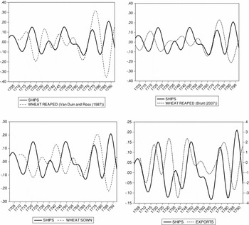
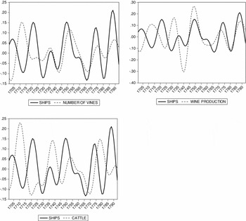
Table 3 involves analysing time-series data adjusted for short-term ‘fluctuations’. However, as argued above, it may be worthwhile to focus on medium-term fluctuations rather than the entire time series. As mentioned in the data section, these fluctuations can be removed in a similar fashion to that employed to extract short-term fluctuations. Figure 9 plots the medium-term fluctuations in wheat production series, including wheat sown and the two wheat reaped estimates of van Duin and Ross (Reference van Duin and Ross1987) and Brunt (Reference Brunt2007), against similar fluctuations in ship traffic. Figure 10 presents similar fluctuations for wine and cattle-related variables.
Medium-term fluctuations in various agricultural production and ship traffic time series

Medium-term fluctuations in viticulture and stock-farming and ship traffic time series

A visual inspection of Figure 9 suggests that medium-run information in wheat production data may be correlated with medium-run information in ship traffic data. Similar econometric analyses are conducted on these medium-term fluctuations to verify the graphical intuition. Table 4 presents the results.
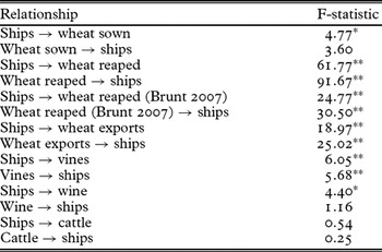
ARDL bounds test results for medium-term fluctuations in agricultural production and ship traffic time series

*Statistically significant at 5% **Statistically significant at 1%
The results differ somewhat from those reported in Table 3. The finding of a statistically significant, bidirectional association between ship traffic and wheat production is maintained. It is particularly important to note that this is true for both the wheat reaped and wheat exported data. As suggested in the literature, there is a systematic relationship between exports and ship traffic. But the relation of wheat production to ship traffic is not limited to wheat exports. We find strong evidence that overall wheat production was systematically related to ship traffic. As mentioned in the data section, we conduct econometric tests for wheat production on both the original van Duin and Ross (Reference van Duin and Ross1987) and the newer Brunt (Reference Brunt2007) estimates, in order to test the extent to which the latter's adjustment affect our conclusions. We reach the same conclusion regardless of data source.
It is interesting to note the difference in results for wheat sown and wheat reaped. While we find a significant relationship between wheat sown and ship traffic, the evidence is weaker than for wheat reaped (compare size of F-statistics). The weaker evidence should not be interpreted as counterevidence: as noted in the data section, the van Duin and Ross (Reference van Duin and Ross1987) and Brunt (Reference Brunt2007) adjustments to the opgaaf data on wheat reaped most likely yielded much improved time-series data on wheat production. Arguably, the higher-quality wheat output data more accurately reflects economic activity in grain production than the uncorrected wheat sown data. We therefore assign greater weight to the relationship suggested by wheat production.
Figure 10 suggests that some of the medium-term fluctuations in wine production series may also be related to medium-term ship traffic fluctuations. Table 4 shows weaker support for a relationship between ship traffic and wine production activities, although our general conclusions are maintained. When using wine production instead of the number of vines as data source, we find some evidence that medium-term fluctuations in ship traffic may be forcing medium-term fluctuations in wine production. The results for the cattle data are generally weaker. In fact, with short-run variation (such as the spikes in cattle numbers in the 1770s and 1780s) removed and long-run information also excluded, it seems that medium-term fluctuations in stock farming activities were not related to ship traffic fluctuations (Figure 10).
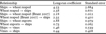
The above findings strongly suggest a bidirectional long-run association between wheat production and ship traffic. However, the fact that both variables appear to adjust to restore equilibrium is not an indication that the relationship was equally strong in both ways. The econometric methodology described earlier can be employed to calculate the size of the long-run relationships between wheat and ship traffic. Table 5 presents these long-run coefficient estimates.
Estimate of long-run correlation between medium-term fluctuations in agricultural production and ship traffic time series

Table 5 supports three important conclusions. First, it shows that the claim for a bidirectional forcing relationship between ship traffic and wheat exports should be interpreted with care. The fluctuations in wheat exports had a much smaller effect on ship traffic fluctuations than the reverse effect of ship traffic on wheat exports. The asymmetric result is consistent with other work, which shows that several other factors influenced ship traffic. First, as shown in Boshoff and Fourie (Reference Boshoff and Fourie2008), ship traffic to the Cape was strongly related to war periods in Western Europe and, second, Dutch ships were required to anchor in Table Bay on their way to the East. Furthermore, while non-Dutch ships were free to bypass the Cape Colony, the lack of substitute ports nearby to provide the level and extent of products and services available in Cape Town is likely to have mitigated the impact of fluctuations in agricultural production on ships’ decisions to visit the Cape. On the other hand, medium-term fluctuations in ship traffic appear to have had an economically and statistically significant effect on medium-term fluctuations in wheat production. The long-run correlation of 2.88 suggests that if ship traffic growth exceeded its long-run trend by 10 per cent, wheat exports also tended to accelerate, growing by 28 per cent in excess of their long-run trend.
The second important conclusion from Table 5 is that ship traffic had an equally large impact on overall wheat production, with a long-run coefficient of around 2.18 using the Brunt (Reference Brunt2007) data. We use the Brunt (Reference Brunt2007) data as the econometric model suggests a better statistical fit (compare the size of standard errors) compared to the fit obtained from the Van Duin and Ross (Reference van Duin and Ross1987) data. As expected, the coefficient estimate of 2.18 is slightly lower than the estimate of 2.88 for wheat exports, given that wheat exports are directly related to ship traffic. Nevertheless, the two coefficient estimates are of a similar size order. This similarity suggests that the impact of ship traffic on agricultural production extended beyond exports: ship traffic in Cape Town harbour not only generated demand for exportable commodities and provisions for ships, but also encouraged agricultural production for local use. Significant long-run increases (or decreases) in ship traffic would have affected inns, pubs, the VOC hospital and many other visitor-related businesses – and their long-run demand for wheat. This is consistent with our argument for the demand-generating impact of travel services consumed in Cape Town.
The third conclusion from Table 5 concerns viticulture. While previous tables suggest a bidirectional relationship, the relationship is clearly more unidirectional in size. Although the evidence is much weaker, the analysis suggests that ship traffic had a long-run correlation coefficient of about 1.46 with the number of vines in the Cape Colony, suggesting that if long-run ship traffic fluctuations exceeded trend by 10 per cent, the trajectory of vines relative to long-run trend would be around 15 per cent. Put the other way around, if ship traffic were to decline below long-run trend growth, one would also see a marked deceleration in the growth rate of vines, with below-trend growth.
The results are conditional given the bivariate nature of the analysis, but they nevertheless suggest that while ship traffic mattered less to in-land activities such as cattle, it was certainly an important driver of economic activity closer to Cape Town, such as wheat and wine production.
Our finding that ships also generated demand for services, apart from exports and ship provisions, relates to a broader debate among economic historians. The literature suggests two explanations for the development of a colonial settlement: first, it is located at a spot suitable for the production of export commodities (the endowment-inequality hypothesis; see Sokoloff and Engerman Reference Sokoloff and Engerman2000; Engerman and Sokoloff Reference Engerman and Sokoloff2002, Reference Engerman and Sokoloff2005); or, second, it offers an abundant supply of land, leading to high real incomes in agriculture, which attracts large numbers of settlers (the settlement of the American territories, for example). The latter was not applicable in the Cape Colony, as immigration was discouraged by the authorities (and slave labour encouraged) and contributed little to the growth in the population (Giliomee Reference Giliomee2003, p. 28). This hypothesis is tested using the same methods described above (see Appendix, Table A1). As expected, we find no medium-run relationship between ship traffic and population growth. The Cape Colony is therefore a unique example of a colonial settlement used for trade purposes, where exports were not limited to commodities, but also included the export of travel services. The strong economic and statistical significance of the coefficients on the relationship between ship traffic and overall wheat production at the Cape – above that of wheat exports – supports this view.
6. Conclusion
The role of settler communities in the economic development of colonial societies has received ample attention in the recent economic history literature. Most notably, the schism between ‘extraction’ versus ‘settler’ European colonies (Acemoglu, Johnson and Robinson Reference Acemoglu, Johnson and Robinson2001) suggests an often artificial severance into two distinct extremes (Austin Reference Austin2008). The Cape Colony of the seventeenth and eighteenth centuries provides a case study of a newly settled, pre-industrial society that does not fit either of these two stereotypes; the Cape settlement was established with the unique purpose of providing refreshment to passing ships on their way from Europe to the East and back. With few local commodities of export value and slow immigration, the Cape of Good Hope was – until fairly recently – considered a backwater with little growth potential, reliant on the passing ships for survival. Van Duin and Ross (Reference van Duin and Ross1987) and Brunt (Reference Brunt2007) challenge this notion, suggesting that the Cape economy yielded relatively strong growth throughout the eighteenth century. They suggest that local demand – and not the passing ships – increased production. If their hypothesis is correct, one would expect little correlation between the (medium-run) fluctuations in ship traffic and agricultural production. Borrowing techniques from the business cycle literature, we test the hypothesis that ship traffic and agricultural production were systematically related. Our findings suggest five broad conclusions.
The first conclusion from the empirical results is that problems with the historical data do influence the analysis. Unadjusted agricultural data do not appear to show any relationship to ship traffic. Furthermore, attempts at signal extraction through moving average smoothing do not appear to address the problem. However, once specific frequency ranges are removed, more supportive evidence emerges. In fact, the second conclusion is that the main hypothesis is supported for wheat and, to a lesser extent, for wine production. There is strong statistical evidence of a bidirectional long-run relationship between wheat production and ship traffic. However, the size of the correlation reveals that ships are more significant in their impact on wheat than vice versa. The evidence for wine production is less convincing and there is partial evidence that ship traffic may have been the stimulating force for viticulture. On the other hand, when also controlling for long-run information (information with a time horizon exceeding 40 years), stock herding fluctuations appear to have been unrelated to ship traffic fluctuations. A third conclusion, therefore, is that agricultural activity closer to Cape Town, in the form of wheat and wine production, appears to have been strongly related to ship traffic, while the relative isolation of the trekboere from more developed Cape Town and its surrounding regions may have contributed to a weaker relationship with ship traffic. A fourth conclusion is related to the impact of exports. In contrast to the work of early historians, exports certainly contributed to economic growth in the Cape Colony. Yet, more importantly, while fluctuations in ship traffic certainly influenced exports, these fluctuations had an even greater effect on overall wheat production. This suggests that the demand created by the ships was not restricted only to goods that could be exported to other settlements, but also stimulated the tertiary sector (to accommodate the thousands of sailors and soldiers arriving annually). The fifth conclusion is therefore that the Cape Colony attained economic growth not only by exporting goods, but also services, to the passing ships. While van Duin and Ross (Reference van Duin and Ross1987) argue correctly that the economy was much more dynamic than historians had previously thought, and even though the number of ships did not experience strong growth during the eighteenth century, their hypothesis that the passing ships on the Cape route had little economic impact should be rejected.
These findings add valuable insights to our understanding of ‘extractive’ colonies. Acemoglu, Johnson and Robinson (Reference Acemoglu, Johnson and Robinson2001) posit that such colonies were set up in ‘places where Europeans faced high mortalisation rates’, while Sokoloff and Engerman (Reference Sokoloff and Engerman2000) argue that extractive industries were set up in areas with specific factor endowments – appropriate climate and soils (including mineral riches) and a large (uneducated) native population. Both theories predict eventual economic underdevelopment. Yet, these conditions did not exist in the dynamic Cape economy, as described by van Duin and Ross (Reference van Duin and Ross1987) and Brunt (Reference Brunt2007). Rather, the Cape Colony developed because of an ‘extractive’, or simply, export sector – including service exports – anchored in the demands of ship traffic. Austin (Reference Austin2008, p. 1021) justifiably criticises these theories – the ‘emphasis on the primacy of a single cause is stimulating but insufficient’ – and calls for more case studies like this one to understand the nuances of development in colonial settlements.
More generally, this article illustrates that techniques developed for the analysis of business cycles can also be applied to the study of fluctuations in a pre-industrial economy. In particular, the band-pass filter can be applied to extract longer-term fluctuations in time series where poor data quality can result in the identification of spurious short-term fluctuations. It also highlights the need to reflect on the contribution of trade, and especially trade-in-services, to the new territories of European discovery. Additionally, the availability of long-run data in the Cape Colony presents researchers with a unique opportunity to empirically investigate the questions of growth and fluctuations in a newly settled, pre-industrial society.
Acknowledgements
The authors wish to thank James Robinson, Jan-Luiten van Zanden, Johannes Fedderke, Grietjie Verhoef, Servaas van der Berg, participants at the 2007 Biennial Conference of the Economic Society of South Africa and 2008 Social Science History Conference in Lisbon and seminar participants at the universities of Cape Town and Stellenbosch for valuable comments and suggestions. Research assistance by Gustav Hendrich, Rina Brink and Harri Kemp, and financial assistance from Economic Research Southern Africa (ERSA) is gratefully acknowledged.
Appendix
ARDL bounds test results for medium-term fluctuations in population and ship traffic time series

*Statistically significant at 5% **Statistically significant at 1%
The results in the table suggest that, while ship traffic certainly affected population, this occurred in the ultra-long run. Medium-run fluctuations in ship arrivals in Cape Town harbour were not directly related to corresponding fluctuations in population figures. This is due to the fact that immigration in the Cape Colony was discouraged for most of the eighteenth century. Furthermore, some settlers arrived in groups (for non-economic reasons), such as the 151 French Huguenots in 1688.