2 Linearization and Local Stability Analysis

The system

$$ \begin{align*} \frac{dx(t)}{dt} &= ax(t-\tau)\bigg( 1-\frac{x(t-\tau)}{k}\bigg) - \frac{bx(t-\tau)y(t)}{x(t-\tau)+1}, \end{align*} $$

$$ \begin{align*} \frac{dy(t)}{dt} &=y(t)\Big( 1-m\frac{y(t)}{nx(t-\tau)+q}-d\Big) \end{align*} $$

has six equilibrium points as $E_1(0,\frac {(1-d)q}{m})$ , $E_2(k,0)$ , $E_3(-1,0)$ , $E_4(0,0)$ , $E_5(x_1^*,y_1^*)$ , and $E_6(x_2^*,y_2^*)$ , where

$$ \begin{align*} x_{1,2}^* = \frac{-\widetilde{B}\pm\sqrt{\widetilde{B^2}-4\widetilde{A}\widetilde{C}}}{2\widetilde{A}} \end{align*} $$

and

$$ \begin{align*} \widetilde{A}&=\frac{a}{k},\\ \widetilde{B}&=\frac{a}{k}-a+\frac{bn(1-d)}{m},\\ \widetilde{C}&=\frac{bq(1-d)}{m}-a, \end{align*} $$

and the corresponding $y_i^*$ is

$$ \begin{align*} y_i^* = \frac{b(1 - d)}{m}(n x_i^* + q). \end{align*} $$

So the system has only one positive equilibrium point $E^*(x^*,y^*)$ when $1-d>0$ and $\widetilde{C}=\frac {bq(1-d)}{m}-a<0$ .

To analyze the local stability of the positive equilibrium point $E^*(x^*,y^*)$ , we first linearize the delayed model and obtain the system

(2.1) $$ \begin{align} \begin{bmatrix} x'(t)\\y'(t) \end{bmatrix} = \operatorname{J_0} \begin{bmatrix} x(t)\\y(t) \end{bmatrix} + \operatorname{J_\tau} \begin{bmatrix} x(t-\tau)\\y(t-\tau) \end{bmatrix}. \end{align} $$

The Jacobian matrices are

$$ \begin{align*} \operatorname{J_0}= \begin{bmatrix} \frac{\partial f}{\partial x}&\frac{\partial f}{\partial y}\\ \frac{\partial g}{\partial x}&\frac{\partial g}{\partial y} \end{bmatrix}_{(x^*,y^*)} , \operatorname{J_\tau}= \begin{bmatrix} \frac{\partial f}{\partial x(t-\tau)}&\frac{\partial f}{\partial y(t-\tau)}\\ \frac{\partial g}{\partial x(t-\tau)}&\frac{\partial g}{\partial y(t-\tau)} \end{bmatrix}_{(x^*,y^*)}, \end{align*} $$

$$ \begin{align*} f(x(t),x(t-\tau),y(t))&=ax(t-\tau)\left(1-\frac{x(t-\tau)}{k}\right)-\frac{bx(t-\tau)y(t)}{x(t-\tau)+1},\\g(x(t),x(t-\tau),y(t))&=y(t)\left(1-m\frac{y(t)}{nx(t-\tau)+q}-d\right). \end{align*} $$

From the partial derivatives of the functions f and g, the Jacobians are

$$ \begin{align*} \operatorname{J_0}= \begin{bmatrix} 0&\frac{-bx(t-\tau)}{x(t-\tau)+1}\\ 0&1+\frac{2my(t)}{nx(t-\tau)+q}-d \end{bmatrix}_{(x^*,y^*)}, \operatorname{J_\tau}= \begin{bmatrix} a-\frac{2ax(t-\tau)}{k}+\frac{by(t)x(t-\tau)}{(x(t-\tau)+1)^2}&0\\ \frac{mny^2(t)}{(nx(t-\tau)+q)^2}&0 \end{bmatrix}_{(x^*,y^*)}. \end{align*} $$

To simplify the matrices, we let

$$ \begin{align*} \operatorname{J_0}_{(x^*,y^*)}= \begin{bmatrix} 0&A_1\\ 0&B_1 \end{bmatrix}, \operatorname{J_\tau}_{(x^*,y^*)}= \begin{bmatrix} C_1&0\\ D_1&0 \end{bmatrix}. \end{align*} $$

$$ \begin{align*} A_1 &= \frac{-bx^*}{x^*+1},\\ B_1 &= 1+\frac{2my^*}{nx^*+q}-d,\\ C_1 &= a-\frac{2ax^*}{k}+\frac{by^*x^*}{(x^*+1)^2},\\ D_1 &= \frac{mny^*{^2}}{(nx^*+q)^2}. \end{align*} $$

When we check the trivial $E_4(0,0)$ equilibrium point for stability at $\tau =0,$ i.e., with no delay

$$ \begin{align*} A_1=0, B_1= 1-d, C_1=a, D_1=0, \\ \lambda^2-(1-d)\lambda-a\lambda e^{-\lambda\tau}+a(1-d)e^{-\lambda\tau}=0,\\ \lambda^2-(1-d+a)\lambda+a(1-d)=0,\\ \lambda_{1,2}= \frac{(1-d+a)\pm\sqrt{(1-d+a)^2-4a(1-d)}}{2}. \end{align*} $$

We observe that for all possible values of $\Delta =(1-d+a)^2-4a(1-d)$ are positive, negative, or zero, the eigenvalues of the corresponding system are always positive or positive real parts, and hence $E_4(0,0)$ equilibrium point is unstable.

Now, for the positive equilibrium point, to find the characteristic equation of the linearized model, we substitute $x = e^{\lambda t}v$ , where $v=\begin {bmatrix} v_1\\ v_2 \end {bmatrix}$ into the system, that is equivalent to

$$ \begin{align*} \lambda e^{\lambda t}v=\operatorname{J_0}e^{\lambda t}v+\operatorname{J_\tau}e^{\lambda(t-\tau)}v , \end{align*} $$

which implies

$$ \begin{align*} \lambda v=\operatorname{J_0}v+\operatorname{J_\tau}e^{-\lambda \tau }v. \end{align*} $$

Then, the corresponding characteristic equation is given by the transcendental equation

(2.2) $$ \begin{align} \quad\operatorname{det(\lambda I-\operatorname{J_0}-\operatorname{J_\tau} e^{-\lambda \tau})=} \begin{vmatrix} \lambda-C_1e^{-\lambda \tau}&-A_1\\ -D_1e^{-\lambda \tau}&\lambda-B_1 \end{vmatrix} =0, \end{align} $$

(2.3) $$ \begin{align} \lambda^2 - B_1 \lambda- C_1 \lambda e^{-\lambda \tau} + (B_1 C_1 - A_1 D_1) e^{-\lambda \tau} = 0. \end{align} $$

When there is no delay, i.e., $\tau =0$ , the corresponding characteristic equation reduces to

(2.4) $$ \begin{align} \lambda^2-(B_1+C_1)\lambda+(B_1C_1-A_1D_1)=0 \end{align} $$

for which $\lambda _{1,2}=\frac {(B_1+C_1)\pm \sqrt {(B_1+C_1)^2-4(B_1C_1-A_1D_1)}}{2}$ . Then, we obtain the following result.

We now examine the distribution of roots of the transcendental equation (2.3), since the stability of point $(0,0)$ of the linearized system (2.1) depends on the locations of the roots of the characteristic equation (2.3). By the continuous dependence of the roots of $\lambda ^2 - B_1 \lambda - C_1 \lambda e^{-\lambda \tau } + (B_1 C_1 - A_1 D_1) e^{-\lambda \tau } = 0$ and Lemma 2.1, there exists $\tau _0> 0$ such that $Re\,\lambda (\tau ^*) < 0$ for $\tau \in [0,\tau _0)$ . Since a loss of asymptotic stability of $E^*(x^*,y^*)$ will arise when $Re\,\lambda (\tau ^*) = 0$ , we shall investigate whether there exists $\tau ^*> 0$ for which $Re\,\lambda (\tau ^*) = 0$ , i.e., we shall decide when equation (2.3) has purely imaginary roots (see [Reference Celik and Çekiç6, Reference Çelik and Merdan8]). Hence, in the next section, we will prove the existence of Hopf bifurcation by finding $\tau _0$ where the system (1.2) loses its asymptotic stability.

3 The Existence of Hopf Bifurcation

To prove the existence of Hopf bifurcation, we first show that the transcendental equation (2.3) has a purely imaginary root by the approach of [Reference Çelik5].

Proof Assume that for $\tau = \tau ^*$ , the characteristic equation (2.3) admits a purely imaginary root $\lambda = i \omega $ , where $\omega $ is a real number, and without loss of generality $\omega> 0$ . Then, we obtain

$$ \begin{align*} (i\omega)^2-C_1i \omega e^{-i\omega \tau}-B_1i\omega+(B_1C_1-A_1D_1)e^{-i\omega \tau}=0. \end{align*} $$

Separating the characteristic equation into its real and imaginary parts leads to:

$$ \begin{align*} -\omega^2-C_1\omega \sin\omega\tau+(B_1C_1-A_1D_1) \cos\omega\tau=0 ,\\-C_1\omega \cos\omega\tau-B_1\omega- (B_1C_1-A_1D_1)\sin\omega\tau=0. \end{align*} $$

To simplify the system of equations, we square both sides of each equation, which yields:

$$ \begin{align*} \omega^4+ C_1^2\omega^2\sin^2\omega\tau+2\omega^3C_1\sin\omega\tau=(B_1C_1-A_1D_1)^2\cos^2\omega\tau,\\B_1^2\omega^2+C_1^2\omega^2\cos^2\omega\tau+2B_1\omega^2C_1\cos\omega\tau=(B_1C_1-A_1D_1)^2\sin^2\omega\tau, \end{align*} $$

(3.1) $$ \begin{align} \omega^4+B_1^2\omega^2-C_1^2(B_1C_1+A_1D_1)^2=0. \end{align} $$

Let

$$ \begin{align*} \omega^2 = z ,\quad p = B_1^2\omega^2,\quad q = -C_1^2(B_1C_1-A_1D_1)^2 , \end{align*} $$

and

(3.2) $$ \begin{align} f(z)=z^2+pz+q. \end{align} $$

Since $\lim _{z\to \infty } f(z) = \infty $ and $q = -C_1^2(B_1C_1-A_1D_1)^2 < 0$ , $f(z)=z^2+pz+q$ has at least one positive root which completes the proof of Lemma 2.1.

By Lemma 2.1, without loss of generality, we denote the positive root by z and $\omega =\sqrt {z}$ . Hence, we obtain

$$ \begin{align*} \omega = \frac{-(B_1^2-C_1^2)\pm\sqrt{(B_1^2-C_1^2)^2+4(B_1C_1-A_1D_1)^2}}{2} \end{align*} $$

and

$$ \begin{align*} \tau_k = \frac{1}{\omega}\!\Bigg[ \arctan \left(\frac{C_1\omega^3+B_1\omega(B_1C_1+A_1D_1)}{A_1D_1\omega^2}\right) + 2k\pi \Bigg],\quad k=0,1,2,\ldots. \end{align*} $$

Denote $\omega _0 = \frac {-(B_1^2-C_1^2)\pm \sqrt {(B_1^2-C_1^2)^2+4(B_1C_1-A_1D_1)^2}}{2}$ and suppose

$$\begin{align*}\lambda_k(\tau) = \alpha_k(\tau) + i \omega_k(\tau) \end{align*}$$

denotes the root of (2.3) near $\tau =\tau _k$ satisfying

$$\begin{align*}\alpha_k(\tau_k) = 0 \quad \text{and} \quad \omega_k(\tau_k) = \omega_0, \quad k = 0,1,2,\dots. \end{align*}$$

Then, we have the following transversality condition.

Lemma 3.2 The following transversality conditions are satisfied:

$$\begin{align*}\frac{d\,\mathrm{Re}(\lambda)}{d\tau}\Big|_{\tau=\tau_k}> 0 \end{align*}$$

$$\begin{align*}\tau = \tau_k, \quad k = 0,1,2,\dots, \end{align*}$$

if $B_1C_1-A_1D_1<0$ , i.e., system (1.1) undergoes Hopf bifurcation at the positive equilibrium point $E^*(x^*,y^*)$ for $\tau = \tau _k, k= 0,1,2\ldots $

Proof Differentiating the characteristic equation (2.3) with respect to $\tau $ , we get

$$ \begin{align*} \frac{d}{d\tau}(\lambda^2-B_1\lambda-C_1\lambda e^{-\lambda\tau}+(B_1C_1-A_1D_1)e^{-\lambda\tau}). \end{align*} $$

$$ \begin{align*} \frac{d\lambda}{d\tau} = \frac{-C_1(\lambda)^2e^{-\lambda\tau}+(B_1C_1-A_1D_1)\lambda e^{-\lambda\tau}}{2\lambda-B_1-C_1e^{-\lambda\tau}+C_1\lambda\tau e^{-\lambda\tau}-(B_1C_1-A_1D_1)\tau e^{-\lambda\tau}}, \end{align*} $$

that is,

$$ \begin{align*} (\frac{d\lambda}{d\tau})^{-1}& = \frac{2\lambda-B_1-C_1e^{-\lambda\tau}+C_1\lambda\tau e^{-\lambda\tau}-(B_1C_1-A_1D_1)\tau e^{-\lambda\tau}}{-C_1(\lambda)^2e^{-\lambda\tau}+(B_1C_1-A_1D_1)\lambda e^{-\lambda\tau}} \\ &=\frac{2\lambda-B_1-C_1e^{-\lambda\tau}-\tau e^{-\lambda\tau}[-C_1\lambda+(B_1C_1-A_1D_1)]}{\lambda e^{-\lambda\tau}[-C_1\lambda+(B_1C_1-A_1D_1)]} \\ &=\frac{2\lambda-B_1-C_1e^{-\lambda\tau}}{\lambda e^{-\lambda\tau}[-C_1\lambda+(B_1C_1-A_1D_1)]}-\frac{\tau}{\lambda}. \end{align*} $$

Thus,

$$ \begin{align*} \operatorname{Re}\!\left(\frac{d\lambda}{d\tau}\right)^{-1}\bigg|_{\lambda=i\omega_0} &= \operatorname{Re}\!\Bigg[ \frac{2i\omega_0-B_1-C_1e^{-i\omega_0\tau}}{[-C_1(i\omega_0)^2 + (B_1C_1 - A_1D_1)(i\omega_0)]e^{-i\omega_0\tau_k}}+\frac{i\tau}{\omega_0}\!\Bigg ]\\&= \operatorname{Re}\!\Bigg[ \frac{2i\omega_0-B_1-C_1(\cos\omega_0\tau-i\sin\omega_0\tau)}{[C_1(\omega_0)^2 + (B_1C_1 - A_1D_1)(i\omega_0)](\cos\omega_0\tau-i\sin\omega_0\tau)}+\frac{i\tau}{\omega_0}\!\Bigg ]\\&=\quad \frac{B_1^2(B_1C_1-A_1D_1)\omega^2+C_1^2\omega^6+2(B_1C_1-A_1D_1)^2\omega^4}{(B_1^2\omega^4+\omega^6)[(B_1C_1-A_1D_1)^2+C_1^2\omega^2]}. \end{align*} $$

The transversality condition, $ \operatorname {Re}\!\left (\frac {d\lambda }{d\tau }\right )\big |_{\lambda =i\omega _0}> 0 $ , if $B_1C_1-A_1D_1<0$ is satisfied. Since both $cos$ and $sin$ take positive values at $x^*$ and $y^*$ , from Rouché’s theorem, we have that the transversality condition holds and the conditions for Hopf bifurcation are satisfied at $\tau = \tau _k$ , $k=0,1,2\ldots $ This completes the proof of the lemma.

Using these results, we can formulate the following theorem describing the stability and Hopf bifurcation behavior of system (1.1).

4 Numerical Simulations

In this section, we present the numerical simulations to verify our theoretical results proved in previous sections by using MATLAB (7.0) programming. Mainly, as an example, we simulate the predator–prey system (1.2) with the parameters, i.e., a = 0.7, b = 0.9, d = 0.6, m = 8, q = 8, n = 9, and k = 6, we consider the following system:

(4.1) $$ \begin{align} \frac{dx(t)}{dt}&=(0.7)x(t-\tau)(1-\frac{x(t-\tau)}{6})-\frac{(0.9)x(t-\tau)y}{x(t-\tau)+1}, \end{align} $$

(4.2) $$ \begin{align} \frac{dy(t)}{dt}&=[1-\frac{8y}{9x(t-\tau)+8}-0.6]y. \end{align} $$

Using the algorithms in previous sections, we obtain that the system (4.1) has only one positive equilibrium point $E^*(x^*, y^*)$ = $(0.467,0.6102)$ . We evaluate that

$$ \begin{align*} \omega_0 = \frac{-(B_1^2 - C_1^2) + \sqrt{(B_1^2 - C_1^2)^2 - 4(B_1 C_1 + A_1 D_1)^2}}{2}, \end{align*} $$

$\omega _0$ = 0.3772 and hence $\tau _0$ = 2.1. According to Theorem 3.3, the equilibrium point $E^*$ is locally asymptotically stable for $\tau \in [0,\tau _0) = [0, 2.1)$ and becomes unstable, when ( $\tau> 2.1$ ). Additionally, a Hopf bifurcation occurs at $\tau =\tau _0=2.1$ as illustrated by the computer simulations. From this, we conclude that the Hopf bifurcation of system (1.1) at $\tau _0 = 2.1$ is supercritical, and a bifurcating periodic solution exists when $\tau $ crosses $\tau _0$ to the right, with the bifurcating periodic solution being unstable. In the computer simulations, we set the initial conditions as $(0.467,0.6102)$ and utilized the MATLAB delay differential equations (DDE) solver to simulate the system described in (1.2). 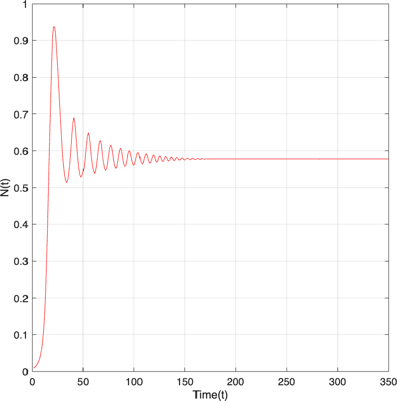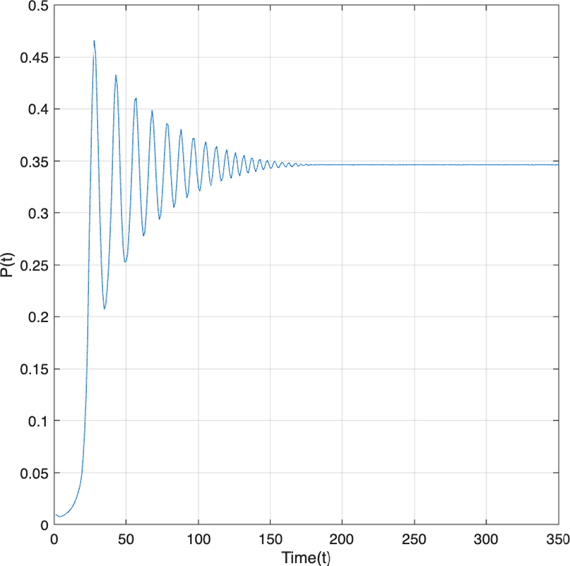Initially, we set $\tau $ = 1.8 $< \tau _0$ and plot the density functions $x(t)$ and $y(t)$ in Figures 1 and 2, respectively, which show that the equilibrium is asymptotically stable for $\tau < \tau _0$ . 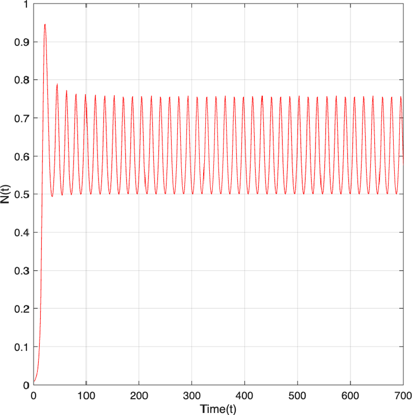In Figures 3 and 4, we set $\tau = 1.8 <\tau _0$ , which is sufficiently close to $\tau _0$ , illustrating the existence of bifurcating periodic solutions from the equilibrium point $E^*$ .

Figure 1

The trajectory of prey density over time is shown for the initial conditions $E^*(x^*, y^*)$ = $(0.467,0.6102)$ . When $\tau = 1.8 < \tau _0,$ where the steady state $E^*$ is asymptotically stable.

Figure 1 Long description

The line graph is plotted on a Cartesian coordinate system with a grid. The horizontal x-axis is labeled Time(t) and ranges from 0 to 350 in increments of 50. The vertical y-axis is labeled N(t) and ranges from 0 to 1 in increments of 0.1.

Data flow:

* The red curve begins near the origin at t = 0.

* It rises sharply to a primary peak of approximately 0.94 at t = 20.

* Following the first peak, the curve undergoes a series of damped oscillations. Each subsequent peak and trough is smaller in amplitude than the previous one.

* The oscillations occur around a central value of approximately 0.58.

* By t = 150, the oscillations become nearly imperceptible.

* From t = 200 to t = 350, the curve becomes a perfectly horizontal line, indicating that the system has reached an asymptotically stable steady state at N(t) approximately equal to 0.58.

Figure 2

The trajectory of the predator density over time is shown for the initial condition $E^*(x^*, y^*) = (0.467, 0.6102)$ . When $\tau = 1.8 < \tau _0$ , the steady state $E^*$ remains stable.

Figure 2 Long description

The graph is plotted on a Cartesian coordinate system with a grid.

* The horizontal x-axis is labeled Time(t) and ranges from 0 to 350 in increments of 50.

* The vertical y-axis is labeled P(t) and ranges from 0 to 0.5 in increments of 0.05.

Data Flow:

* The trajectory begins near the origin at t = 0 with a very low P(t) value.

* Between t = 0 and t = 25, there is a sharp exponential-like increase.

* Starting around t = 25, the curve enters a phase of damped oscillations. The first and highest peak reaches approximately 0.47, followed by a trough at 0.21.

* As time progresses toward t = 150, the amplitude of the oscillations decreases significantly.

* By t = 180, the oscillations cease, and the line becomes perfectly horizontal, indicating convergence to a steady state at a P(t) value of approximately 0.347. This stability continues through the end of the plot at t = 350.

Figure 3

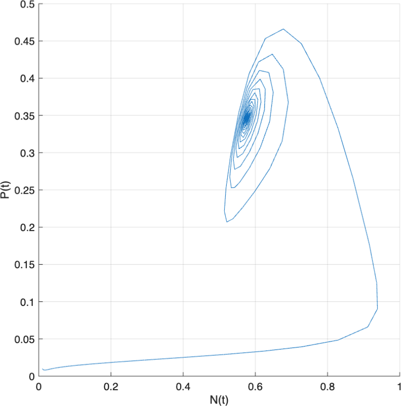
The trajectory and phase portrait corresponding to the initial condition $E^*(x^*, y^*) = (0.467, 0.6102)$ are presented. For $\tau = 1.8 < \tau _0$ , the steady state $E^*$ is asymptotically stable.

Figure 3 Long description

The line graph is plotted on a Cartesian coordinate system with a grid. The horizontal x-axis is labeled N(t) with values ranging from 0 to 1 in increments of 0.2. The vertical y-axis is labeled P(t) with values ranging from 0 to 0.5 in increments of 0.05.

A single blue trajectory line begins near the origin at approximately (0.01, 0.01). It moves horizontally to the right along the bottom of the graph until it reaches N(t) approximately 0.9. From there, it curves sharply upward and to the left, forming a large outer loop that peaks at P(t) approximately 0.47 and N(t) approximately 0.68.

The trajectory then continues to spiral inward in a clockwise direction. Each subsequent loop is smaller than the last, indicating an asymptotic approach to a central point. The spiral eventually converges and becomes highly dense at a steady state located at approximately N(t) equals 0.6 and P(t) equals 0.35.

Figure 4

The trajectory of prey density over time is shown for the initial conditions $E^*(x^*, y^*)$ = $(0.467,0.6102)$ . When $ \tau =2.1,$ where the steady state $E^*$ is converging.

5 Discussion and conclusion

In this study, we analyze the dynamics of a ratio-dependent predator–prey system incorporating a discrete time delay. The model exhibits a single positive equilibrium point $E^*(x^*, y^*) = (0.467, 0.6102)$ . Through linearization and the derivation of the characteristic equation, we establish the conditions under which the system undergoes a Hopf bifurcation. 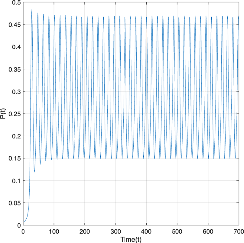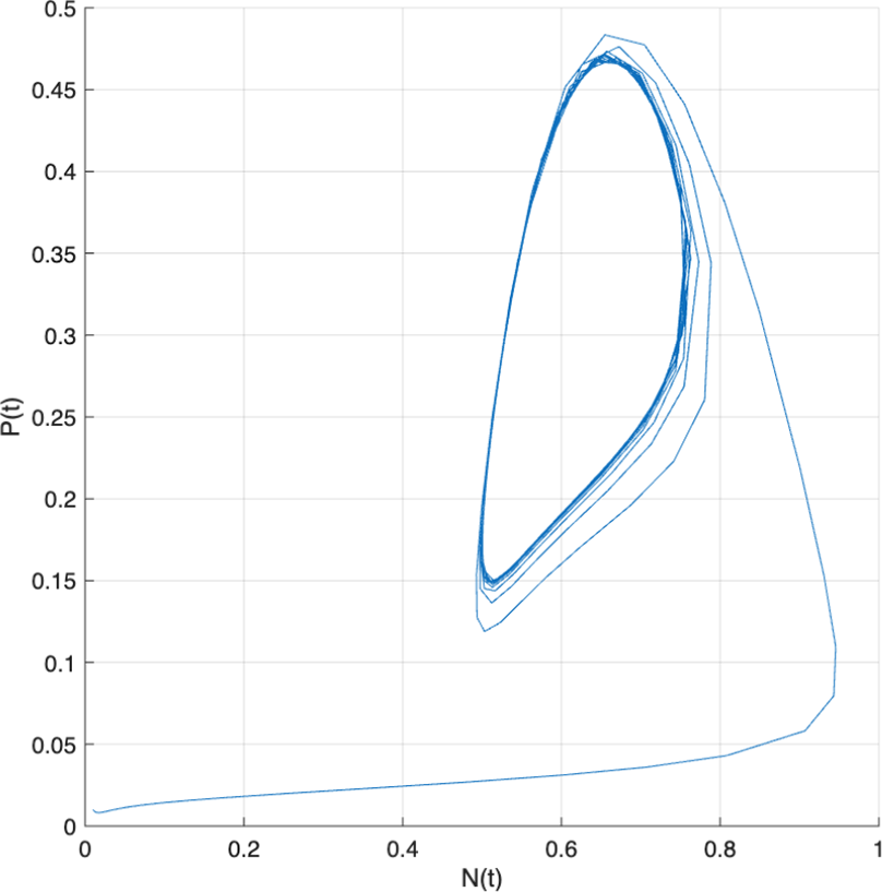The corresponding transversality condition is verified, confirming the existence of a critical delay value $\tau _0 = 2.1$ at which the system transitions from asymptotic stability to instability. Figure 5 illustrates the dynamical behavior of the system for the chosen parameter values for the predator densities. Figure 6 presents the phase portrait corresponding to the analytical results (Figures 5 and 6).

Figure 5

The trajectory of predator density over time is shown for the initial conditions $E^*(x^*, y^*)$ = $(0.467,0.6102)$ . When $ \tau =2.1,$ where the steady state $E^*$ is converging.

Figure 6

The trajectory and phase portrait corresponding to the initial conditions $E^*(x^*, y^*)$ = $(0.467, 0.6102)$ . When $\tau =2.1,$ where the steady state $E^*$ is converging.

Numerical simulations conduct in MATLAB’s DDE solver further validate the theoretical findings. When $\tau = 1.8$ ( $\tau < \tau _0$ ), the equilibrium $E^*$ remains asymptotically stable, as shown in Figures 1 and 2. Conversely, for $\tau = 2.1$ ( $\tau> \tau _0$ ), the system exhibits periodic oscillations emerging from $E^*$ , consistent with the onset of a Hopf bifurcation, as illustrated in Figures 3 and 4. These results demonstrate the sensitivity of the system to variations in the delay parameter and highlight how time delays can induce complex oscillatory behavior in predator–prey interactions.

The Hopf bifurcation observed at $\tau _0 = 2.1$ is found to be supercritical, implying that a stable periodic solution bifurcates from the equilibrium point as the delay parameter surpasses the critical threshold. This finding underscores the importance of time delays in ecological modeling, where delayed feedback mechanisms often play a pivotal role in generating sustained population oscillations.

The analysis presents here builds upon classical approaches used in delay-differential models, such as the Holling–Tanner, Leslie–Gower, and Michaelis–Menten type systems [Reference Çelik5, Reference Karaoglu and Merdan11]. Our results align with previous studies [Reference Celik and Çekiç6, Reference Çelik and Merdan8], further supporting the robustness of Hopf bifurcation theory in capturing the transition from equilibrium stability to periodic behavior in biological systems.

Overall, the study provides both theoretical and computational evidence for the occurrence of a supercritical Hopf bifurcation in the delayed predator–prey model. The findings contribute to a deeper understanding of how delay-dependent mechanisms influence ecological stability and periodicity. Future research may extend this framework to multi-delay systems or investigate the impact of stochastic perturbations and parameter uncertainty on the bifurcation structure, enhancing the model’s applicability to real-world ecosystems.