1 Introduction
Convective flow caused by an unstable stratification of fluid density such as the Rayleigh–Bénard or the Rayleigh–Taylor instabilities is common in porous media. The Rayleigh–Bénard instability appears when an unstable density stratification is maintained between the top and bottom boundaries of the domain. This is often found when the fluid temperature is altered as in geothermal groundwater systems (Cheng Reference Cheng1979; Sanford, Whitaker & Smart Reference Sanford, Whitaker, Smart and Jones1998) and heat conduction in metallic foams (Dyga & Troniewski Reference Dyga and Troniewski2015; Hamadouche, Nebbali & Benahmed Reference Hamadouche, Nebbali, Benahmed, Kouidri and Bousri2016) or during the mixing of freshwater and seawater in coastal aquifers (Cooper Reference Cooper1964; Abarca, Carrera & Sánchez-Vila Reference Abarca, Carrera, Sánchez-Vila and Voss2007). The Rayleigh–Taylor instability occurs when one fluid is placed on top of a less dense one. A situation found in geological CO
 $_{2}$
storage (Ennis-King & Paterson Reference Ennis-King and Paterson2005; Szulczewski, Hesse & Juanes Reference Szulczewski, Hesse and Juanes2013), the displacement of dense contaminant plumes (Kueper & Frind Reference Kueper and Frind1991) or the convection of compositional melts (Martin, Griffiths & Campbell Reference Martin, Griffiths and Campbell1987; Tait & Jaupart Reference Tait and Jaupart1989; Wells, Wettlaufer & Orszag Reference Wells, Wettlaufer and Orszag2011). The coupling between flow and transport results in an enhancement of boundary and dissolution fluxes and fluid mixing. Since mixing leads to the attenuation of concentration contrasts and dilution (Kitanidis Reference Kitanidis1994; Dentz, Le Borgne & Englert Reference Dentz, Le Borgne, Englert and Bijeljic2011; Le Borgne, Dentz & Villermaux Reference Le Borgne, Dentz and Villermaux2015) and drives chemical reactions (De Simoni, Carrera & Sánchez-Vila Reference De Simoni, Carrera, Sánchez-Vila and Guadagnini2005; Dentz et al.
Reference Dentz, Le Borgne, Englert and Bijeljic2011), understanding how unstable flow and mixing interact is therefore essential to predict the behaviour of such systems.
The behaviour of mixing and dissolution fluxes is usually expressed in terms of dimensionless quantities. In Rayleigh–Bénard instabilities, the fluxes are represented by the Nusselt number
 $\mathit{Nu}$
(see Otero, Dontcheva & Johnston Reference Otero, Dontcheva, Johnston, Worthing, Kurganov, Petrova and Doering2004) and depend on the strength of the instability given by the Rayleigh number
 $\mathit{Ra}$
. The numerical simulations of Otero et al. (Reference Otero, Dontcheva, Johnston, Worthing, Kurganov, Petrova and Doering2004) found
 $\mathit{Nu}\propto \mathit{Ra}^{0.9}$
for
 $1300\lesssim \mathit{Ra}\lesssim 10\,000$
. Hewitt, Neufeld & Lister (Reference Hewitt, Neufeld and Lister2012) found exponents close to 1 for
 $\mathit{Ra}>1000$
. These observations are in agreement with the boundary layer analysis of Howard (Reference Howard1966) that assumes that the buoyancy flux is independent of the height of the domain. Although the low
 $\mathit{Ra}$
regime is not discussed, inspection of figure 3 in Otero et al. (Reference Otero, Dontcheva, Johnston, Worthing, Kurganov, Petrova and Doering2004) and figure 2 in Hewitt et al. (Reference Hewitt, Neufeld and Lister2012) shows that
 $\mathit{Nu}\propto \mathit{Ra}^{1/2}$
for
 $100\lesssim \mathit{Ra}\lesssim 1000$
, which differs from the
 $\mathit{Nu}\propto \mathit{Ra}^{2/3}$
predicted by Kimura, Schubert & Straus (Reference Kimura, Schubert and Straus1986).
Rayleigh–Taylor instabilities also display different scaling depending on the dominant mechanism (Slim Reference Slim2014). The system evolves from
 $\mathit{Nu}\propto \mathit{Ra}^{1/2}$
when diffusion dominates to
 $\mathit{Nu}\propto \mathit{Ra}$
after the onset of the instabilities (Hidalgo, Fe & Cueto-Felgueroso Reference Hidalgo, Fe, Cueto-Felgueroso and Juanes2012; Hidalgo et al. Reference Hidalgo, Dentz, Cabeza and Carrera2015). In bounded domains, as the instabilities attenuate, the relation between
 $\mathit{Nu}$
and
 $\mathit{Ra}$
becomes time dependent (Hewitt, Neufeld & Lister Reference Hewitt, Neufeld and Lister2013a
; Hidalgo et al.
Reference Hidalgo, Dentz, Cabeza and Carrera2015).
We focus on the behaviour of dissolution fluxes and fluid mixing in the presence of convective flow. Mixing in unstable systems occurs at the fluid interfaces, which can be located at the domain boundaries or at the contact with another fluid and whose shape is determined by the instability patterns. The patterns organize themselves into cells, columnar plumes or fingers, and evolve jointly with the velocity field, which forms vortices and stagnation points. The fluid interface is stretched and compressed at these locations, especially at stagnation points, affecting the magnitude of the fluxes across it.
We study the hydrodynamic mechanisms of convective mixing and dissolution and quantify them in an interface compression model that is able to reproduce the observed mixing scaling. The model relates the structure of the velocity field to mixing and dissolution fluxes across the fluid interface. First, we present the governing equations of the flow and transport in porous media and define the observables that describe the system, namely, the scalar dissipation rate and concentration probability density function and discuss their relation to dissolution fluxes and mixing state of the system. Then we introduce the interface compression model for the mixing and dissolution fluxes in the vicinity of a stagnation point. We consider three scenarios with increasing complexity. A double-gyre synthetic velocity which is used to validate the interface compression model, a heat transport problem in which a Rayleigh–Bénard instability is triggered by the boundary conditions, and a two-fluid system in which the density stratification provokes a Rayleigh–Taylor instability. The interface compression model shows how mixing is controlled by the structure of the velocity field, whose properties determine the transition between scalings.
2 Flow and transport governing equations
Under the assumptions of incompressible fluids and the Boussinesq approximation, the dimensionless governing equations for variable-density single-phase flow in a two-dimensional (2-D) homogeneous porous medium are (Riaz, Hesse & Tchelepi Reference Riaz, Hesse, Tchelepi and Orr2006; Hidalgo, MacMinn & Juanes Reference Hidalgo, MacMinn and Juanes2013):
 $$\begin{eqnarray}\displaystyle & \displaystyle \unicode[STIX]{x1D735}\boldsymbol{\cdot }\boldsymbol{q}=0, & \displaystyle\end{eqnarray}$$
 $$\begin{eqnarray}\displaystyle & \displaystyle \boldsymbol{q}=-\unicode[STIX]{x1D735}p+\unicode[STIX]{x1D70C}(c)\hat{\boldsymbol{e}}_{g}, & \displaystyle\end{eqnarray}$$
 $$\begin{eqnarray}\displaystyle & \displaystyle \frac{\unicode[STIX]{x2202}c}{\unicode[STIX]{x2202}t}+\boldsymbol{q}\boldsymbol{\cdot }\unicode[STIX]{x1D735}c-\frac{1}{\mathit{Ra}}\unicode[STIX]{x1D6FB}^{2}c=0, & \displaystyle\end{eqnarray}$$
where
 $p$
is a scaled pressure referred to a hydrostatic datum,
 $\boldsymbol{q}$
is the dimensionless Darcy velocity and
 $\hat{\boldsymbol{e}}_{g}$
is a unit vector in the direction of gravity. The dimensionless density
 $\unicode[STIX]{x1D70C}$
is in general a function of concentration
 $c$
. Choosing as time scale the advective characteristic time
 $t_{a}=L_{c}/q_{c}\unicode[STIX]{x1D719}$
, where
 $L_{c}$
is the system length scale,
 $\unicode[STIX]{x1D719}$
the porosity and
 $q_{c}=k\unicode[STIX]{x1D70C}_{c}g/\unicode[STIX]{x1D707}$
the characteristic buoyancy velocity given by the permeability
 $k$
, viscosity
 $\unicode[STIX]{x1D707}$
, a representative density
 $\unicode[STIX]{x1D70C}_{c}$
and gravity
 $g$
, the transport equation (2.3) is controlled only by the Rayleigh number
 $$\begin{eqnarray}\displaystyle & \displaystyle \mathit{Ra}=\frac{q_{c}L_{c}}{\unicode[STIX]{x1D719}D_{m}}, & \displaystyle\end{eqnarray}$$
where
 $D_{m}$
is the diffusion coefficient. The different scales must be chosen depending on the problem solved and will be explained when necessary.
The system behaviour is analysed in terms of the global scalar dissipation rate
 $$\begin{eqnarray}\displaystyle & \displaystyle \langle \unicode[STIX]{x1D712}\rangle =\frac{1}{\mathit{Ra}}\int _{\unicode[STIX]{x1D6FA}}\text{d}\unicode[STIX]{x1D6FA}\,|\unicode[STIX]{x1D735}c|^{2}, & \displaystyle\end{eqnarray}$$
where
 $\unicode[STIX]{x1D6FA}$
denotes the domain. At the steady state,
 $\langle \unicode[STIX]{x1D712}\rangle$
is equal to the flux through the boundaries (Hidalgo et al.
Reference Hidalgo, Fe, Cueto-Felgueroso and Juanes2012) and since
 $\mathit{Nu}$
is defined as the flux divided by the diffusive flux over the domain (
 $1/\mathit{Ra}$
in the current setup), it can be seen that
 $\langle \unicode[STIX]{x1D712}\rangle =\mathit{Nu}/\mathit{Ra}$
.
In closed systems the change of concentration variance (Le Borgne, Dentz & Bolster Reference Le Borgne, Dentz, Bolster, Carrera, de Dreuzy and Davy2010) is equal to
 $2\langle \unicode[STIX]{x1D712}\rangle$
. As the system mixes and concentration homogenizes
 $\langle \unicode[STIX]{x1D712}\rangle$
goes to zero. However, in the presence of sinks or sources the concentration variance is also related to the boundary or dissolution fluxes (Hidalgo et al.
Reference Hidalgo, Fe, Cueto-Felgueroso and Juanes2012). In that case a non-zero
 $\langle \unicode[STIX]{x1D712}\rangle$
proportional to the fluxes can be found in the steady state. In that case the mixing state of the system is better represented by the probability density function (p.d.f.) of the concentration calculated by sampling the concentration in all the domain as
 $$\begin{eqnarray}\displaystyle & \displaystyle p(c)=\frac{1}{A}\int _{\unicode[STIX]{x1D6FA}}\unicode[STIX]{x1D6FF}[c-c(\boldsymbol{x})]\,\text{d}\unicode[STIX]{x1D6FA}, & \displaystyle\end{eqnarray}$$
where and
 $A$
is the domain’s area.
The shape of
 $p(c)$
when the system is well mixed depends on the boundary conditions. For example, for a well-mixed closed system,
 $p(c)$
is given by a Dirac delta centred at the average initial concentration. If Dirichlet boundary conditions maintain a concentration difference between the system’s boundaries and diffusion is the only transport mechanism, the concentration profile is linear and the p.d.f. flat. Segregated systems are characterized by broad concentration p.d.f.s with multiple local maxima.
To obtain information about the spatial structure we shall use the two-dimensional autocorrelation function
 $$\begin{eqnarray}\displaystyle & \displaystyle \text{ACF}_{g}(\boldsymbol{x})={\mathcal{F}}^{-1}\left\{\left|{\mathcal{F}}\{g(\boldsymbol{x})\}\right|^{2}\right\}, & \displaystyle\end{eqnarray}$$
where
 $g(\boldsymbol{x})$
is the function whose autocorrelation is computed and
 ${\mathcal{F}}$
stands for the two-dimensional Fourier transform. The shape of ACF indicates the presence of periodic structures. The correlation length
 $l$
is related to the width of the first maximum of the ACF and gives information about the size of those structures.
3 Interface compression
After the onset of instabilities, the fluid interface evolves under the combined effect of velocity and diffusion (Elder Reference Elder1968). In the locations where the velocity field experiences sharp changes, such as the stagnation points where the flow velocity goes to zero over a distance equal to the interface thickness, the interface is compressed and stretched. Diffusion, however, has the opposite effect and acts to increase the interface width. The thickness
 $s$
of the interfacial boundary layer is the result of the competition between hydrodynamic compression and diffusive expansion, which can be quantified by (Villermaux Reference Villermaux2012; Le Borgne, Dentz & Villermaux Reference Le Borgne, Dentz and Villermaux2013)
 $$\begin{eqnarray}\displaystyle & \displaystyle \frac{1}{s}\frac{\text{d}s}{\text{d}t}=-\unicode[STIX]{x1D6FE}+\frac{1}{\mathit{Ra}}\frac{1}{s^{2}}, & \displaystyle\end{eqnarray}$$
with
 $\unicode[STIX]{x1D6FE}$
the dimensionless compression rate and the dimensionless diffusion coefficient
 $\mathit{Ra}^{-1}$
. The compression rate is given by the symmetric part of the strain tensor (Ottino Reference Ottino1989)
 $$\begin{eqnarray}\unicode[STIX]{x1D640}=\frac{1}{2}(\unicode[STIX]{x1D735}\boldsymbol{q}+\unicode[STIX]{x1D735}\boldsymbol{q}^{\text{T}})=\left[\begin{array}{@{}cc@{}}\unicode[STIX]{x1D6FE} & 0\\ 0 & -\unicode[STIX]{x1D6FE}\end{array}\right].\end{eqnarray}$$
The steady state solution of (3.1) determines the length scale
 $$\begin{eqnarray}\displaystyle & \displaystyle s_{B}=\frac{1}{\sqrt{\unicode[STIX]{x1D6FE}\mathit{Ra}}} & \displaystyle\end{eqnarray}$$
at which the effects of compression and diffusion equilibrate. This length is known as the Batchelor scale (Batchelor Reference Batchelor1959; Villermaux & Duplat Reference Villermaux and Duplat2006).
In general the scalar transport in the vicinity of a stagnation point located at a fluid interface can be described by the advection–diffusion equation (Ranz Reference Ranz1979; Villermaux Reference Villermaux2012; Le Borgne et al. Reference Le Borgne, Dentz and Villermaux2013; Hidalgo et al. Reference Hidalgo, Dentz, Cabeza and Carrera2015)
 $$\begin{eqnarray}\displaystyle & \displaystyle \frac{\unicode[STIX]{x2202}c}{\unicode[STIX]{x2202}t}=\unicode[STIX]{x1D6FE}z\frac{\unicode[STIX]{x2202}c}{\unicode[STIX]{x2202}z}+\frac{1}{\mathit{Ra}}\frac{\unicode[STIX]{x2202}^{2}c}{\unicode[STIX]{x2202}z^{2}}, & \displaystyle\end{eqnarray}$$
where horizontal gradients are disregarded because they are small along the interface and the stagnation point is located at
 $z=0$
. Following Hidalgo et al. (Reference Hidalgo, Dentz, Cabeza and Carrera2015), the steady state solution for
 $c$
along its characteristics gives
 $$\begin{eqnarray}\displaystyle & \displaystyle c=c_{b}+\frac{1-c_{b}}{2}\text{erfc}\left(\frac{z}{\sqrt{2s_{B}^{2}}}\right), & \displaystyle\end{eqnarray}$$
where it is considered that the concentration far above the interface (
 $z\rightarrow -\infty$
) is 1 and far below the interface (
 $z\rightarrow \infty$
) has a value
 $c_{b}$
, which can be different from zero.
Using (3.5) in (2.5) we obtain the expression for
 $\langle \unicode[STIX]{x1D712}\rangle$
 $$\begin{eqnarray}\displaystyle & \displaystyle \langle \unicode[STIX]{x1D712}\rangle =\frac{\unicode[STIX]{x1D714}_{e}}{\sqrt{4\unicode[STIX]{x03C0}}}\frac{(1-c_{b})^{2}}{s_{B}\,\mathit{Ra}}, & \displaystyle\end{eqnarray}$$
where
 $\unicode[STIX]{x1D714}_{e}$
denotes an effective interface length in the horizontal direction. The form of
 $\unicode[STIX]{x1D714}_{e}$
depends on the characteristics of the flow and will be discussed for each of the considered scenarios.
4 Mixing around a stagnation point: the double gyre
To illustrate the interface compression model we analyse the behaviour of fluxes and mixing using a double-gyre velocity field (Shadden, Lekien & Marsden Reference Shadden, Lekien and Marsden2005). This a simplified model of convective flow, because flow and transport are uncoupled, and flow around stagnation points. Similar models have been used to characterize mixing in oceanic circulation (Musgrave Reference Musgrave1985).
4.1 Double gyre
We consider a rectangular domain of length 2 and height 1 in which the incompressible velocity
 $\boldsymbol{q}=(q_{x},q_{z})$
is given by
 $$\begin{eqnarray}\displaystyle & \displaystyle q_{x}=\sin (n\unicode[STIX]{x03C0}x)\cos (\unicode[STIX]{x03C0}z)/n & \displaystyle\end{eqnarray}$$
 $$\begin{eqnarray}\displaystyle & \displaystyle q_{z}=-\cos (n\unicode[STIX]{x03C0}x)\sin (\unicode[STIX]{x03C0}z), & \displaystyle\end{eqnarray}$$
where
 $n$
is a positive integer equal to 1 for the double gyre. Concentration is prescribed on top and bottom boundaries so that
 $$\begin{eqnarray}\displaystyle c(x,z)=\left\{\begin{array}{@{}c@{}}0,\quad \text{at }z=0,\\ 1,\quad \text{at }z=1,\end{array}\right.\end{eqnarray}$$
and the lateral boundaries are periodic. Density is constant and flow and transport are not coupled. There is no characteristic buoyancy velocity, so we take
 $q_{c}=\max (q_{z})=1$
and
 $\mathit{Ra}=q_{c}L_{c}/\unicode[STIX]{x1D719}D_{m}$
, which is in fact a Péclet number since the velocity field is not related to convective instabilities.
4.2 Interface compression and scalar dissipation
The velocity field varies smoothly along the vertical direction, compresses the fluid against the top boundary and maintains the concentration gradient. The structure of the velocity field can also be visualized through the determinant of
 $|\unicode[STIX]{x1D640}|$
, which displays extremes at the stagnation points. The velocity 2-D autocorrelation also reveals the periodicity of the velocity field (figure 1
d).
(a–d) Steady state concentration and velocity field (arrows) for the double gyre
 $(\mathit{Ra}=5000)$
, determinant of the strain tensor
 $\unicode[STIX]{x1D640}$
, magnitude of the velocity and 2-D normalized autocorrelation of the velocity field. The autocorrelation is computed using the Wiener–Khinchin theorem and results are shifted so that the maximum is at the centre of the domain.

There are eight stagnation points in the domain (figure 1). At the steady state only the ones at the boundaries contribute to mixing because the concentration gradients inside the domain are zero. We take the one at the centre of the top boundary where the interface is compressed for the calculations. The compression rate at that point is
 $\unicode[STIX]{x1D6FE}=\unicode[STIX]{x03C0}$
and (3.3) gives
 $s_{B}=\sqrt{1/\unicode[STIX]{x03C0}\mathit{Ra}}$
. Therefore from (3.6) we obtain
 $$\begin{eqnarray}\displaystyle & \displaystyle \langle \unicode[STIX]{x1D712}\rangle \sim \frac{1}{2\sqrt{\mathit{Ra}}}. & \displaystyle\end{eqnarray}$$
The
 $\mathit{Ra}^{-1/2}$
dependence was observed by Ching & Lo (Reference Ching and Lo2001) for similar velocity fields. In the double gyre, the velocity changes in a scale of the order of the domain and
 $\unicode[STIX]{x1D6FE}$
is therefore independent of the value of
 $\mathit{Ra}$
. Thus the
 $\mathit{Ra}^{-1/2}$
behaviour is characteristic of systems in which the velocity field (and
 $\unicode[STIX]{x1D6FE}$
) and diffusion are uncoupled.
To verify the stagnation point model, we solved the double-gyre transport problem for
 $500<\mathit{Ra}<20\,000$
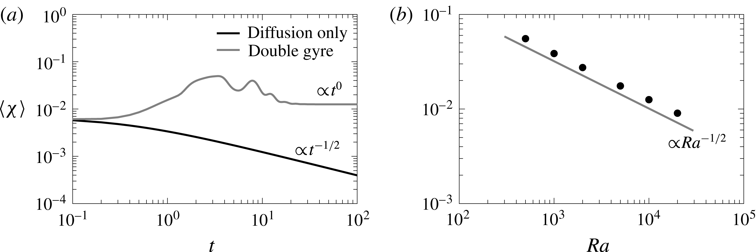
. As expected, the effect of the convection increases the mixing efficiency of the system (figure 2
a), which arrives to a steady state much faster than the diffusion only case. The global scalar dissipation rate displays the expected
 $\mathit{Ra}^{-1/2}$
behaviour (figure 2
b).
(a) Comparison between a diffusion only case (black solid line), that is velocity equal zero, and the case with a double-gyre velocity field for
 $\mathit{Ra}=10\,000$
(grey solid line). The global scalar dissipation rate scales as
 $t^{-1/2}$
for late times in the diffusion case while the double gyre evolves to a constant behaviour. (b) Dependence of the total mixing
 $\langle \unicode[STIX]{x1D712}\rangle$
with
 $\mathit{Ra}$
for the double gyre.

As time passes the interface is compressed at the stagnation point until the compression of the velocity field is balanced by diffusion and the width equilibrates at the Batchelor scale
 $s_{B}$
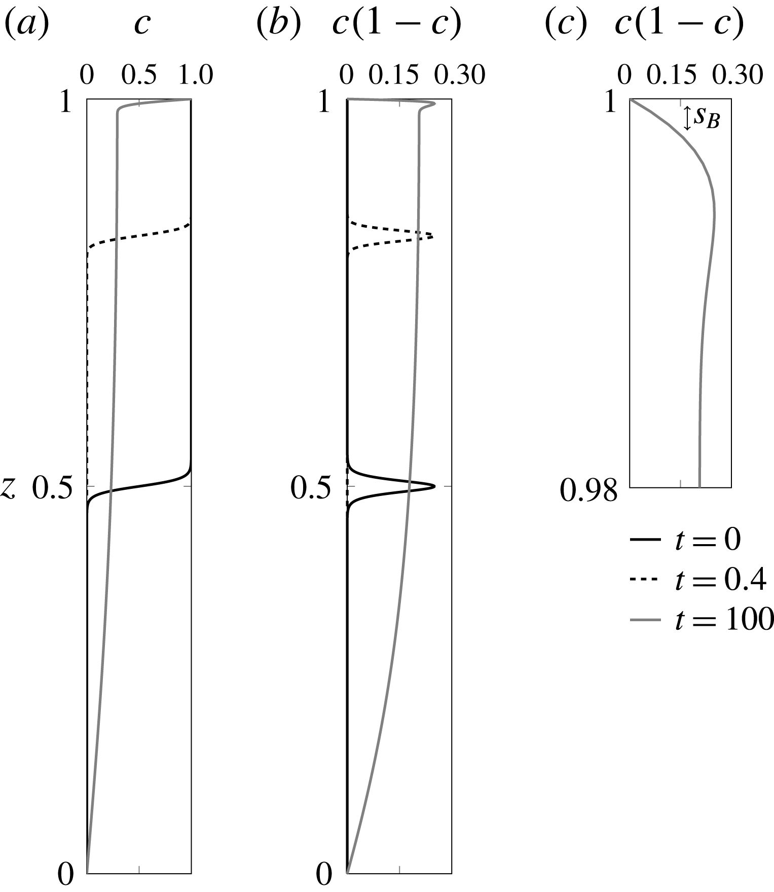
. The interface width can be estimated as the square root of the second central moment (variance) of
 $c(1-c)$
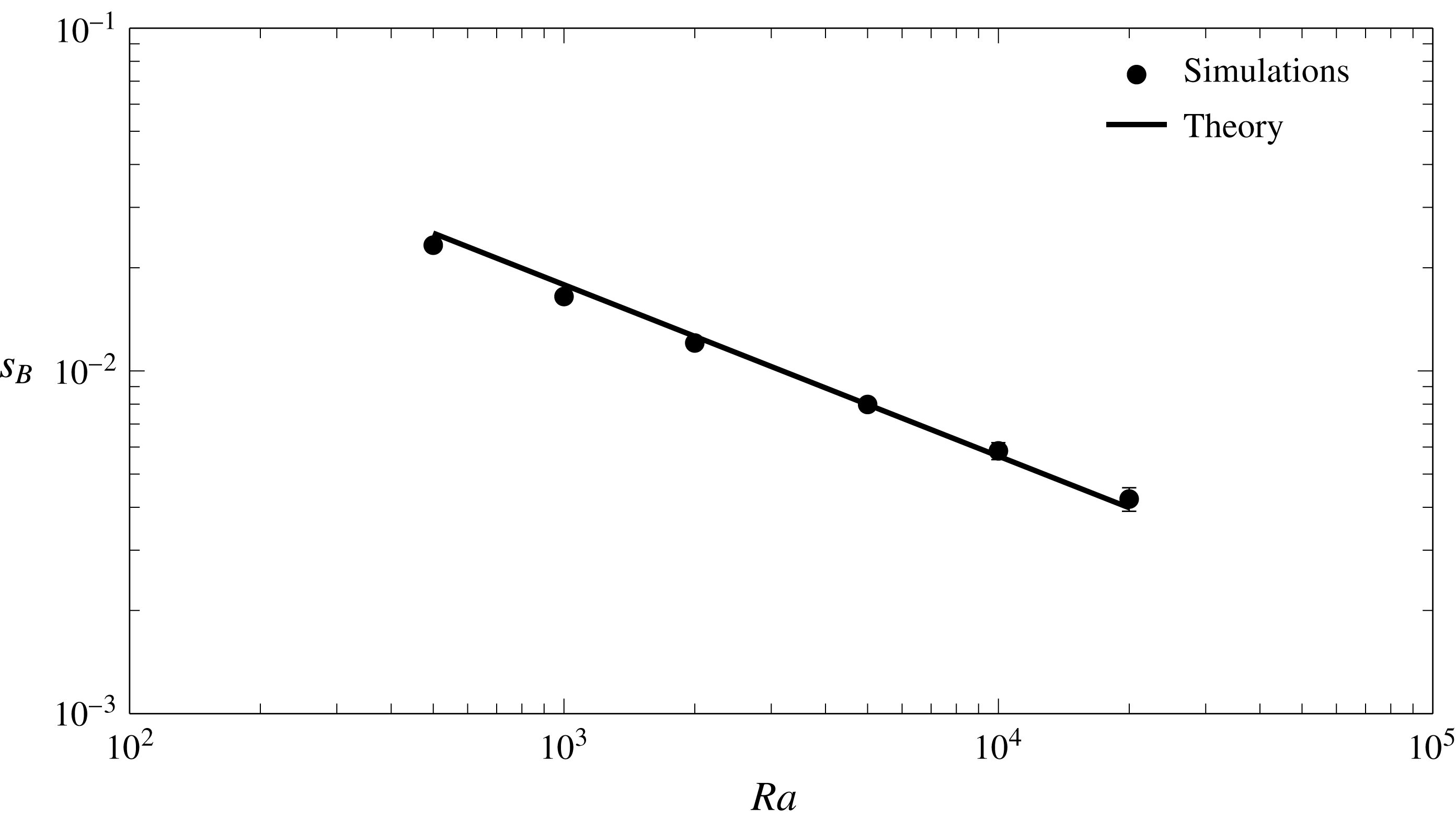
at the stagnation point as illustrated in figure 3. There is a good agreement between the theoretical Batchelor scale and the numerical model (figure 4).
(a) Concentration profile and (b,c)
 $c(1-c)$
of the concentration for the double gyre (
 $n=1$
) at
 $x=0.5$
for times
 $t=0,0.4,100$
. It can be seen how the interface is compressed against the top and bottom boundary as the system approaches steady state. The decrease in the interface width is shown by the shape of
 $c(1-c)$
.

Computed (dots) interface width at the stagnation point and theoretical (solid line) Batchelor scale (
 $s_{B}=(\unicode[STIX]{x03C0}\mathit{Ra})^{-1/2}$
).

The number of stagnation points
 $n_{sp}$
and convection cells in the system increases with
 $n$
. There are
 $2n-1$
convection cells and
 $2n$
stagnation points where the interface is compressed. The compression rate at the stagnation points is independent of
 $n$
and so is
 $\max (q_{z})$
. Therefore,
 $\mathit{Ra}$
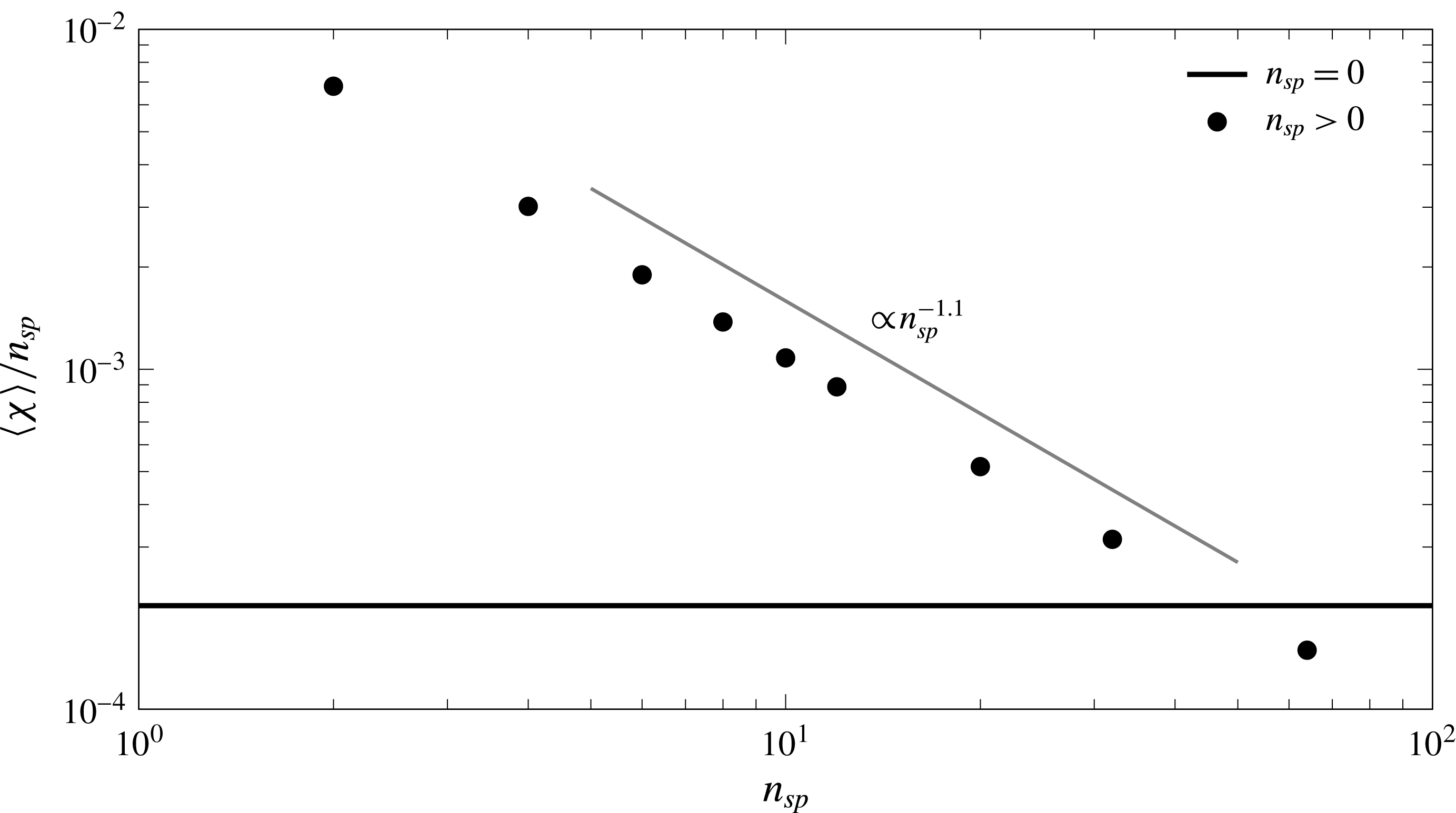
does not change. The simulations show that
 $\langle \unicode[STIX]{x1D712}\rangle$
decreases with the number of cells (figure 5). The decrease of dissolution efficiency per stagnation point is caused by a reduction in the width of the cells. This reduction behaves as
 $n^{-1}$
in good agreement with the numerical results.
Global scalar dissipation rate with increasing number of stagnation points
 $n_{sp}$
for
 $\mathit{Ra}=10\,000$
. The solid horizontal line corresponds to the case in which diffusion is the only transport mechanism (
 $n_{sp}=0$
).

4.3 Mixing state
The mixing state of the system is represented by the concentration p.d.f.
 $p(c)$
and its variance
 $\unicode[STIX]{x1D70E}_{c}^{2}$
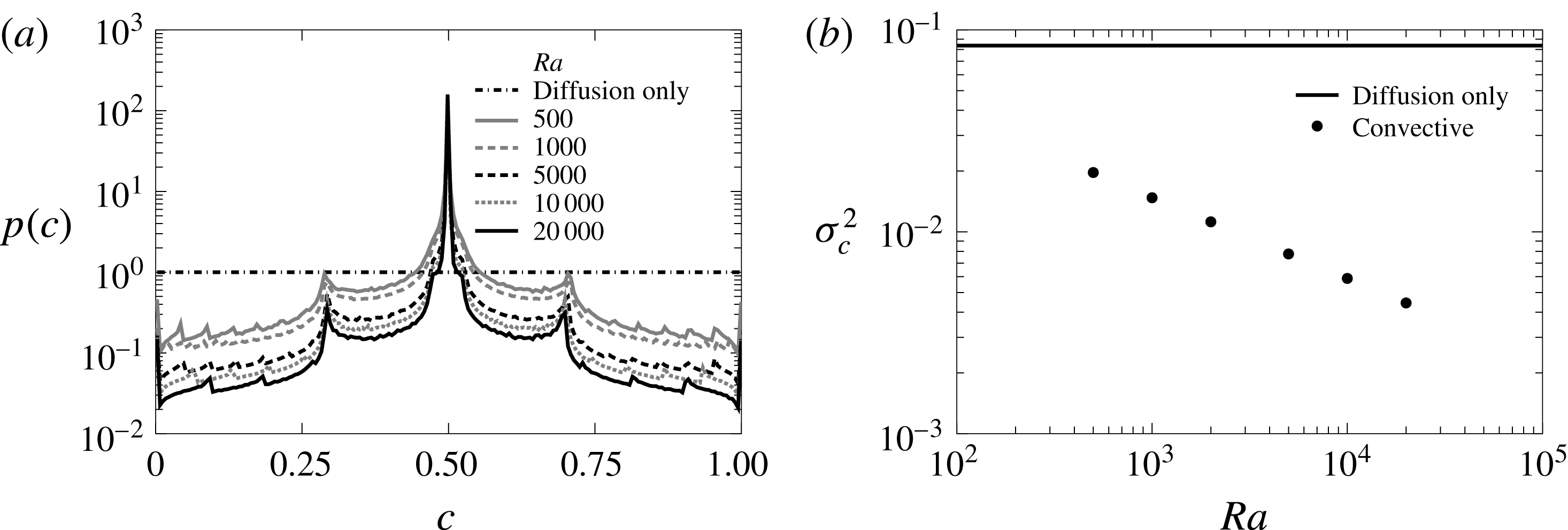
, which also shows the effect of convection. Without convection the p.d.f. (figure 6
a) is uniform for all the concentration range because the concentration profile is linear. As
 $\mathit{Ra}$
increases and the well-mixed area inside the convection cells grows and the concentration differences are confined near the boundaries. The weight of the extreme concentration decreases and the p.d.f. sharpens around the mean value of
 $0.5$
. The peaks at
 $c=0$
and
 $c=1$
corresponding to the boundary conditions are always visible. The secondary peaks correspond to the areas around the stagnation points near the boundaries where the mean concentration is in between that of the boundary and the well-mixed zone inside the cells.
Convection also helps in making the system more homogeneous. When diffusion is the only mixing mechanism
 $p(c)$
has the maximum variance possible because all values of concentration are equiprobable (figure 6
b). The concentration variance
 $\unicode[STIX]{x1D70E}_{c}^{2}$
is inversely proportional to
 $\mathit{Ra}$
reflecting the above-mentioned reduction of the area occupied by concentration gradients.
Steady state concentration p.d.f. for the double-gyre case (
 $n=1$
) and different values of
 $\mathit{Ra}$
(a) and the p.d.f. variance (b). The diffusion only case is computed with
 $\mathit{Ra}=10\,000$
.

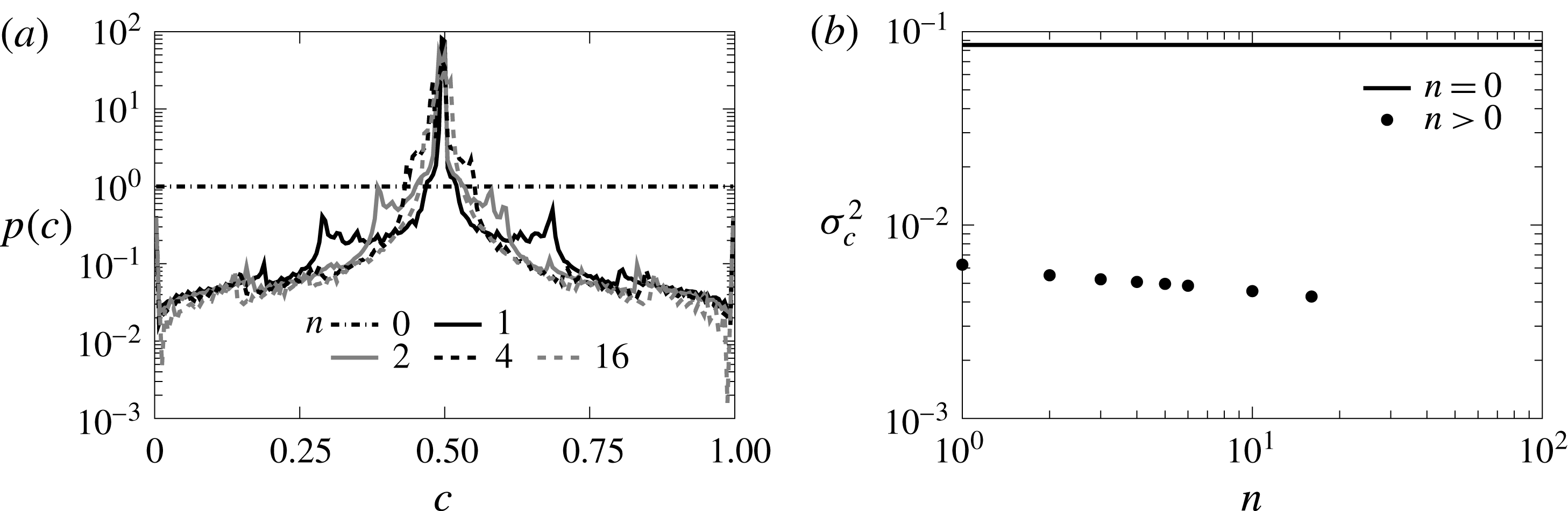
The number of cells also affects the system state. The concentration p.d.f. displays a sharper shape (figure 7
a) and the number of secondary peaks increases with
 $n$
. The stirring of additional convection cells, however, does not improve the homogeneity of the steady state system significantly. The variance of concentration (figure 7
b) is not reduced significantly by the addition of more cells. It is interesting to note that the higher the dissolution flux, i.e. higher
 $\langle \unicode[STIX]{x1D712}\rangle$
, the less well mixed the system is.
Concentration p.d.f. (a) and variance (b) for the multiple-gyre case for different values of
 $n$
and
 $\mathit{Ra}=10\,000$
. The velocity field homogenizes the system. However, the efficiency above
 $n=1$
decreases significantly.

5 Mixing across immobile interfaces
We consider now a system for which the instabilities originate at the boundary and propagate to the rest of the finite domain. The interface is then fixed on one side and the shape of the instability patterns is constrained in principle by the geometry of the system.
5.1 The Horton–Rogers–Lapwood problem
The Horton–Rogers–Lapwood (HRL) problem (Horton & Rogers Reference Horton and Rogers1945; Lapwood Reference Lapwood1948) is a heat transport problem in which convection is triggered by a Rayleigh–Bénard instability caused by the temperature difference between the top and bottom boundaries. We solve the problem in a rectangular domain of aspect ratio 2 (as in the double-gyre case) with impervious top and bottom boundaries and periodic boundary conditions on the sides. Temperature
 $T=1$
is prescribed at the top boundary and
 $T=0$
at the bottom one. The dimensionless density of the fluid increases linearly with temperature as
 $\unicode[STIX]{x1D70C}=\unicode[STIX]{x1D6FD}T$
, where
 $\unicode[STIX]{x1D6FD}$
is a positive constant. The system is again characterized by the Rayleigh number (2.4), which in this case takes the form
 $\mathit{Ra}=k\unicode[STIX]{x1D6FD}L_{c}/\unicode[STIX]{x1D719}\unicode[STIX]{x1D707}D_{m}$
since
 $q_{c}=k\unicode[STIX]{x1D6FD}/\unicode[STIX]{x1D707}$
.
The system is stable for
 $\mathit{Ra}<4\unicode[STIX]{x03C0}^{2}$
. For
 $4\unicode[STIX]{x03C0}^{2}\lesssim \mathit{Ra}\lesssim 1300$
(Graham & Steen Reference Graham and Steen1994) the instability patterns occupy the whole domain in the form of convection cells (figure 8). For higher
 $\mathit{Ra}$
the system evolves to a chaotic convection regime in which flow is organized in columnar patterns (Hewitt, Neufeld & Lister Reference Hewitt, Neufeld and Lister2013b
). This transition occurs around
 $\mathit{Ra}_{c}\sim 1300$
, which will be called critical Rayleigh number in the following.
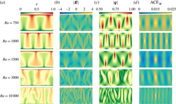
(a–d) Concentration, determinant of the strain tensor
 $\unicode[STIX]{x1D640}$
, modulus of the velocity and 2-D normalized autocorrelation of the velocity field for the Horton–Rogers–Lapwood problem and different
 $\mathit{Ra}$
at time
 $t=1000$
. The autocorrelation is computed using the Wiener–Khinchin theorem and results are shifted so that the maximum is at the centre of the domain.

The stagnation points in this problem are located at the top and bottom boundaries (figure 8). For moderate
 $\mathit{Ra}$
they are found in between the convection cells and remain stationary once the convection is fully developed. For high
 $\mathit{Ra}$
when the system experiences chaotic convection, the stagnation points are located at the boundaries from where the columnar plumes grow. They appear and disappear along the boundary as the small proto-plumes merge and interact.
5.2 Interface compression and scalar dissipation
The global scalar dissipation rate
 $\langle \unicode[STIX]{x1D712}\rangle$
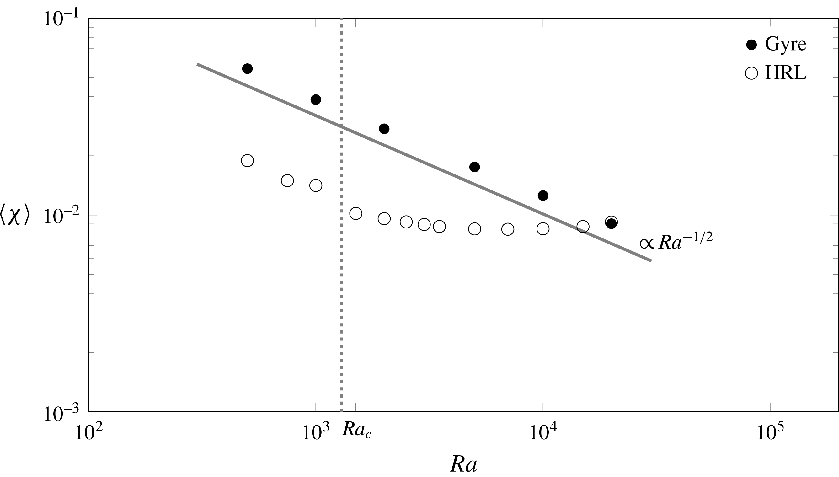
reflects the transition of the system from an uncoupled, self-organized, convective regime, in which
 $\langle \unicode[STIX]{x1D712}\rangle \propto \mathit{Ra}^{-1/2}$
as in the double-gyre scenario, to a convection dominated regime characterized by
 $\langle \unicode[STIX]{x1D712}\rangle \propto \mathit{Ra}^{0}$
(figure 9). The origin of this change in the system’s behaviour lies in the structure of the velocity field. As shown in figure 8, for low
 $\mathit{Ra}$
the strain and the velocity field resemble that of the double gyre as the similarities in velocity and velocity autocorrelation indicate. The velocity structure is dominated by the convection pattern, which depends on the size and aspect ratio of the domain. Therefore the velocity changes happen in the scale of the domain size, as in the double-gyre case, and the compression rate is independent of
 $\mathit{Ra}$
. In the convection dominated regime, however, the size of the domain becomes unimportant because the mixing process happens at the scale of the interface, which is of the order of the Batchelor scale. Velocity changes across a distance of the order of
 $s_{B}$
and
 $\unicode[STIX]{x1D6FE}$
grows linearly with
 $\mathit{Ra}$
. That is, compression and diffusion become coupled.
Dependence of the global scalar dissipation rate on the Rayleigh number for the double-gyre system and the Horton–Rogers–Lapwood (HRL) problem. Mixing for HRL problem changes its behaviour from uncoupled (
 $\propto \mathit{Ra}^{-1/2}$
) to convective around the critical Rayleigh number. This behaviour has also been observed by Otero et al. (Reference Otero, Dontcheva, Johnston, Worthing, Kurganov, Petrova and Doering2004) and Hewitt et al. (Reference Hewitt, Neufeld and Lister2012).

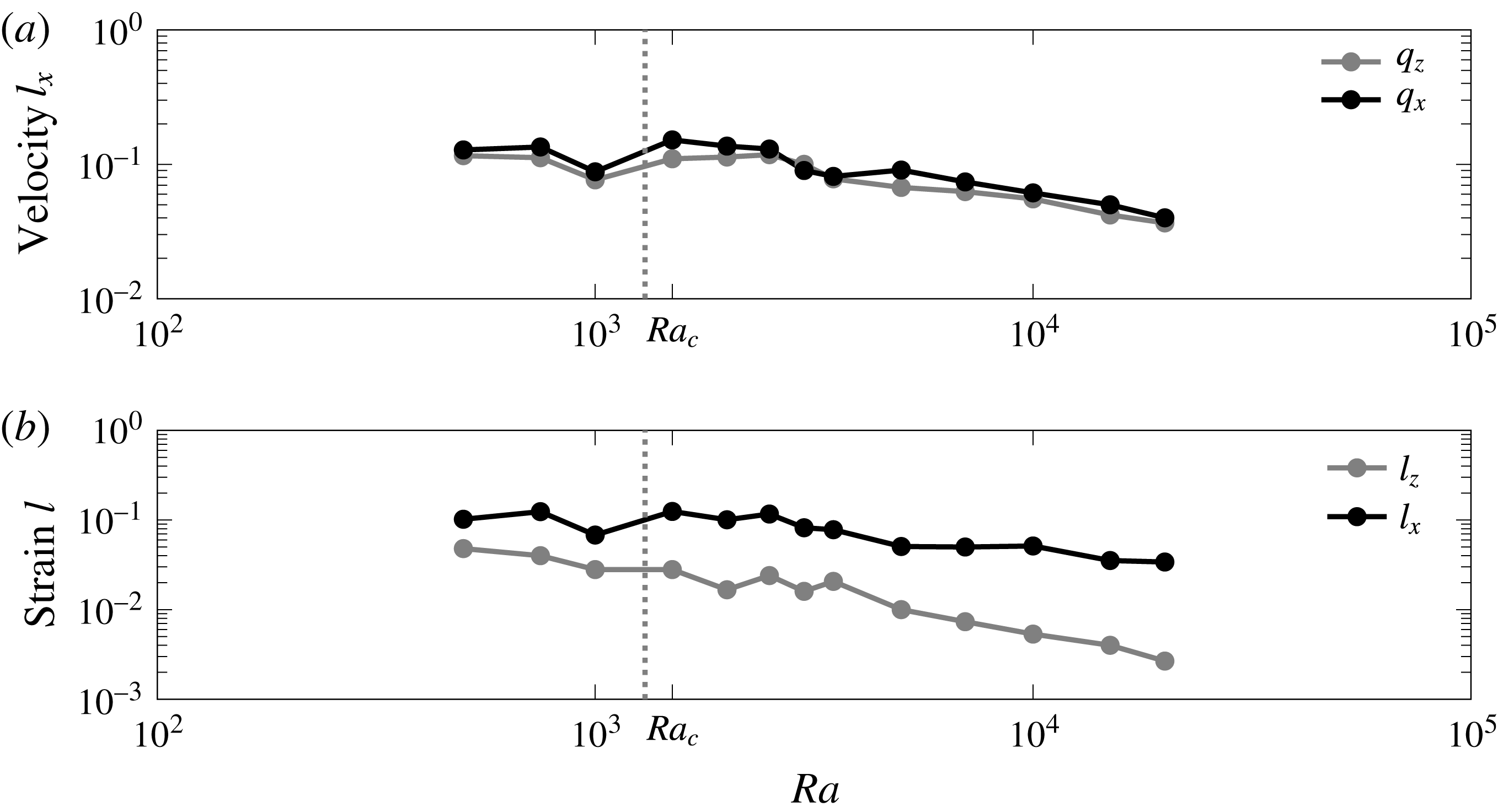
This change in behaviour is reflected in the correlation length in the horizontal direction of the velocity and the strain. The correlation length depends on the number of convection cells for
 $\mathit{Ra}<\mathit{Ra}_{c}$
. When a new cell is created as happens between
 $\mathit{Ra}=750$
(2 cells, see figure 8) and
 $\mathit{Ra}=1000$
(3 cells) the correlation length decreases (figure 10). It increases again when
 $\mathit{Ra}=1500$
and the system has two cells again. For
 $\mathit{Ra}>\mathit{Ra}_{c}$
the correlation lengths decrease rapidly, indicating the transition to the convective dominated regime.
Horton–Rogers–Lapwood problem velocity correlation length in the horizontal direction for both components of the velocity (a) and strain correlation length in both directions (b). The correlation length is computed using the magnitudes averaged from
 $t=20$
to
 $t=100$
.

The interface compression model (3.1)–(3.6) explains the observed behaviours of
 $\langle \unicode[STIX]{x1D712}\rangle$
in the different regimes based on the scalings of the compression rate
 $\unicode[STIX]{x1D6FE}$
. Regardless of the regime, the difference in concentration across the interface at the steady state is the one between the boundaries, that is
 $c_{b}=0$
. The effective length
 $\unicode[STIX]{x1D714}_{e}$
associated with the stagnation points during first regime is weakly dependent on
 $\mathit{Ra}$
because it is linked to the number of convection cells, which oscillates between 2 and 3 (figure 8). The compression rate is, as explained before, independent of
 $\mathit{Ra}$
. Therefore from (3.3) and (3.6) we obtain
 $s_{B},\langle \unicode[STIX]{x1D712}\rangle \propto \mathit{Ra}^{-1/2}$
.
During the convection dominated regime velocity changes sharply across the interface thickness,
 $\unicode[STIX]{x1D6FE}\sim 1/s_{B}$
and (3.3) yields
 $s_{B}\sim \mathit{Ra}^{-1}$
. The effective length
 $\unicode[STIX]{x1D714}_{e}$
is independent of
 $\mathit{Ra}$
because it is proportional to the number of stagnation points
 $({\sim}\mathit{Ra})$
times their individual effective length, which is proportional to the wavelength of the most unstable mode
 $({\sim}\mathit{Ra}^{-1})$
(Riaz et al.
Reference Riaz, Hesse, Tchelepi and Orr2006; Hidalgo et al.
Reference Hidalgo, Dentz, Cabeza and Carrera2015). Therefore from (3.6) we obtain
 $\langle \unicode[STIX]{x1D712}\rangle \sim \mathit{Ra}^{0}$
.
Numerical simulations confirm the former analysis. As in the double-gyre case, we define the interface width as the square root of the second central moment of
 $c(1-c)$
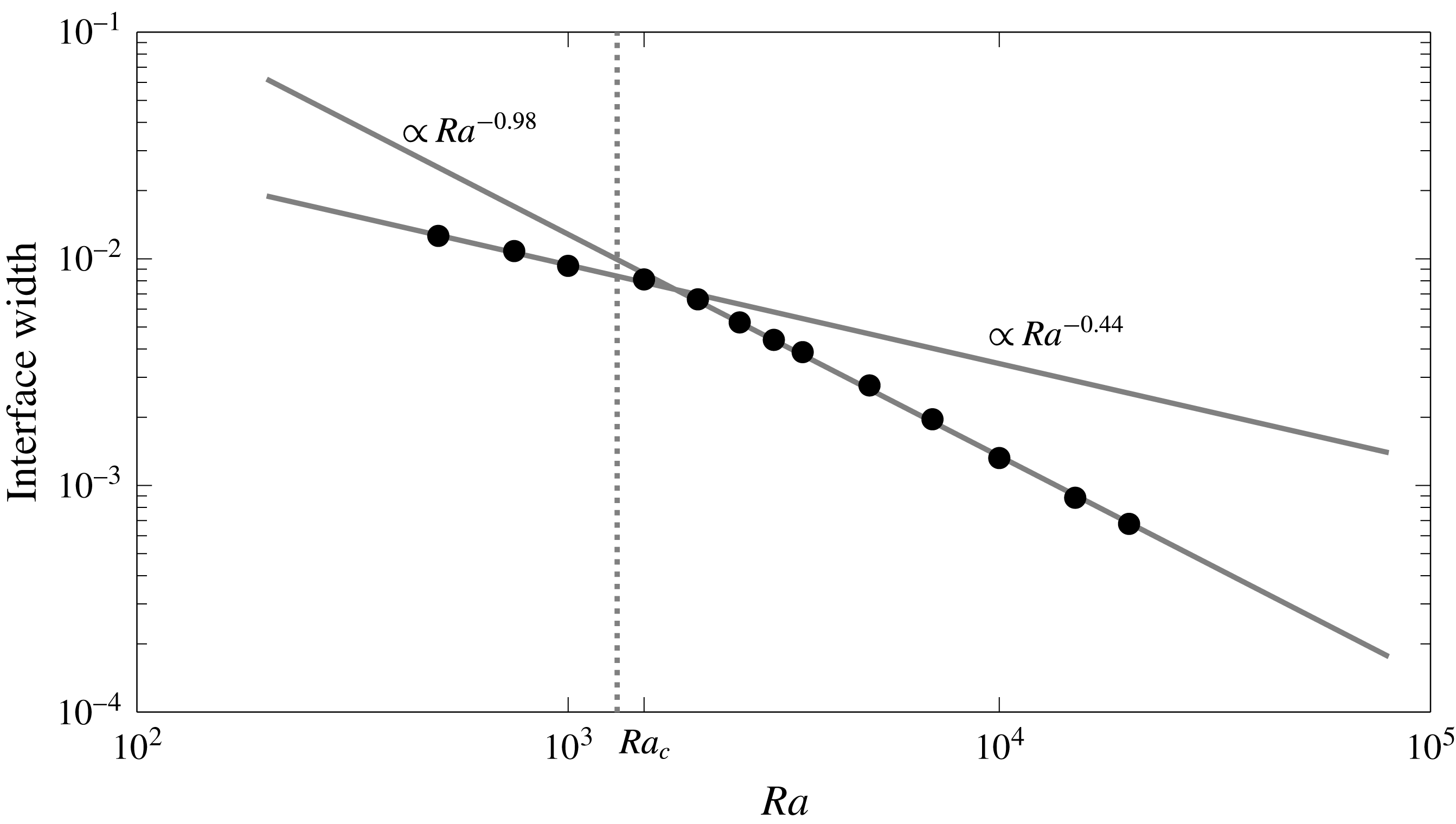
. We compute the second central moment at all locations along the top boundary and take as representative of the interface width the minimum measured value since the movement along the boundary of the stagnation point and the alternation of places where the interface is compressed leads to a time average that overestimates the interface width. We observe (figure 11) that there is a change in the scaling of the interface width around
 $\mathit{Ra}_{c}$
from a value close to the
 $\mathit{Ra}^{-1/2}$
predicted by the model to a
 $\mathit{Ra}^{-1}$
value virtually equal to the model prediction and the observations in previous works (Rees, Selim & Ennis-King Reference Rees, Selim, Ennis-King and Vadasz2008; Hidalgo & Carrera Reference Hidalgo and Carrera2009; Slim & Ramakrishnan Reference Slim and Ramakrishnan2010; Hewitt et al.
Reference Hewitt, Neufeld and Lister2013a
).
Interface width dependence on
 $\mathit{Ra}$
for the Horton–Rogers–Lapwood problem. The width is computed as the average between
 $t=20$
and
 $t=100$
of the minimum along the horizontal direction of the square root of the second central moment of
 $c(1-c)$
.

5.3 Mixing state
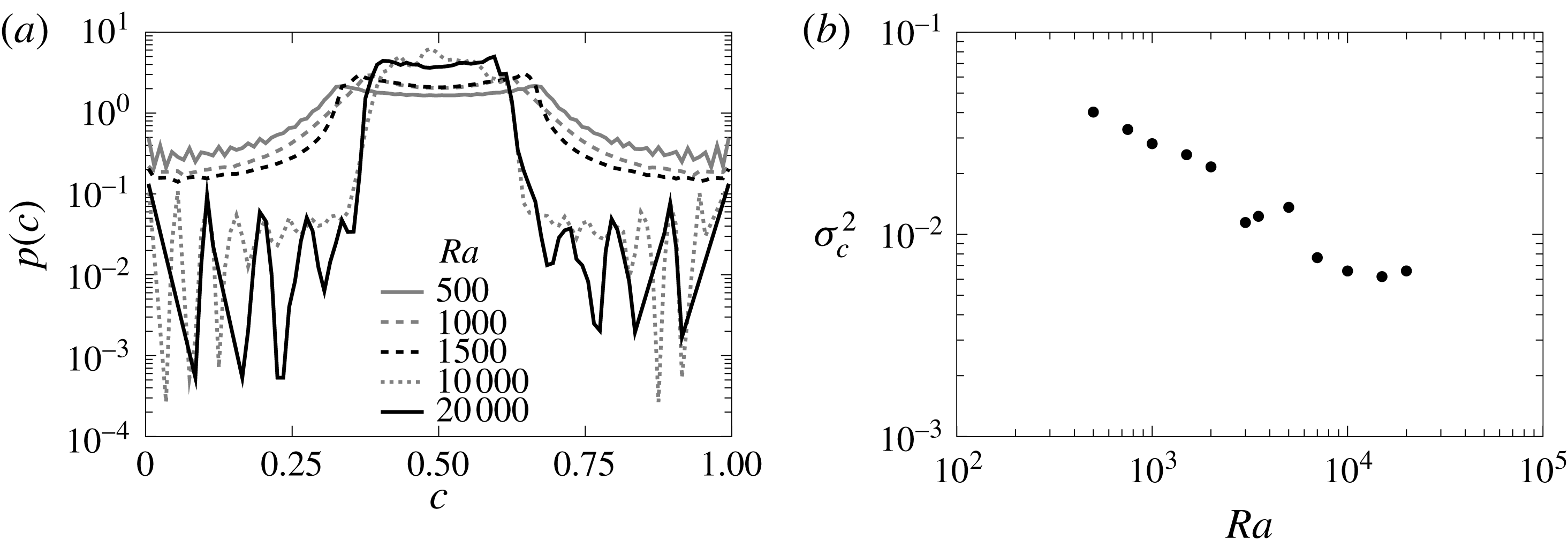
Similarly to the double-gyre case the increasing strength of convection narrows the concentration p.d.f. around the average concentration
 $c=0.5$
(figure 12
a). However,
 $p(c)$
is not as sharp as in the double-gyre case because the area between the convection cells or columnar plumes where the fluid is well mixed is smaller. This area grows as
 $\mathit{Ra}$
increases, which leads to a smaller concentration variance (figure 12
b) and a more homogeneous system.
Contrary to the scalar dissipation rate
 $\langle \unicode[STIX]{x1D712}\rangle$
, which is dominated by the concentration gradients at the interface, the mixing state of the system does not become independent of
 $\mathit{Ra}$
as the system passes to the chaotic convection regime. The decrease in mixing efficiency happens around
 $\mathit{Ra}\approx 10\,000$
, which is one order of magnitude bigger than
 $\mathit{Ra}_{c}$
.
The dependence of
 $\unicode[STIX]{x1D70E}_{c}^{2}$
on
 $\mathit{Ra}$
implies an in principle counter-intuitive behaviour: mixing increases with reducing diffusion. The responsible for this behaviour is the increasingly chaotic convection, which stirs the system below the interface more efficiently than the convection cells, and leads together with a decreasing but finite diffusion to a more efficient homogenization of the mixture.
Probability density function of the time averaged concentration for the HRL problem (a) and p.d.f. variance (b). Concentration was averaged from
 $t=20$
to
 $t=100$
. Colours indicate different
 $\mathit{Ra}$
. For high
 $\mathit{Ra}$
the p.d.f.s display some noise for the extreme values of concentration.

6 Stagnation points at mobile interfaces
In stratified fluid systems the interface between the fluids is not stationary and in general does not remain flat (Hewitt et al. Reference Hewitt, Neufeld and Lister2013a ). We relax now the assumption of a fixed flat interface and analyse a system subject to a Rayleigh–Taylor instability triggered by an unstable stratification of fluids. The interface compression and mixing model for this system was previously developed by Hidalgo et al. (Reference Hidalgo, Dentz, Cabeza and Carrera2015), which we further discuss below.
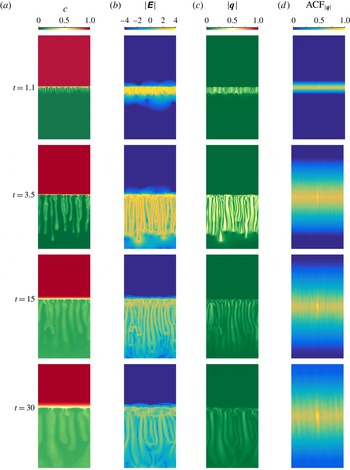
(a–d) Concentration, determinant of the strain tensor
 $\unicode[STIX]{x1D640}$
, modulus of the velocity and 2-D normalized autocorrelation of the velocity field for the two-fluid system under a Rayleigh–Taylor instability for
 $\mathit{Ra}=10\,000$
at different times.

6.1 Rayleigh–Taylor instability
We consider a rectangular domain of length 1 and height 2 with top and bottom impervious boundaries and periodic boundary conditions on the sides (figure 13). Initially the system is in equilibrium with a less dense fluid on top of a dense one with the interface located at
 $z=1$
. The fluids are fully miscible. Instabilities are triggered by a fluid nonlinear non-monotonic density law based on the mixtures of propylene-glycol and water (Backhaus, Turitsyn & Ecke Reference Backhaus, Turitsyn and Ecke2011; Dow Chemical 2011) which is approximated in dimensionless form by
 $\unicode[STIX]{x1D70C}(c)=6.19c^{3}-17.86c^{2}+8.07c$
(Hidalgo et al.
Reference Hidalgo, Dentz, Cabeza and Carrera2015). Note that the dimensionless density is zero for
 $c=0$
(bottom fluid) and negative for
 $c=1$
(top fluid). The maximum density is found at
 $c_{m}=0.26$
so that the mixture of the fluids is denser than any of the pure ones (Neufeld, Hesse & Riaz Reference Neufeld, Hesse, Riaz, Hallworth, Tchelepi and Huppert2010; Hidalgo et al.
Reference Hidalgo, Fe, Cueto-Felgueroso and Juanes2012, Reference Hidalgo, Dentz, Cabeza and Carrera2015). Again, the system is completely characterized by the Rayleigh number (2.4) defined with
 $q_{c}=k\unicode[STIX]{x0394}\unicode[STIX]{x1D70C}gH_{0}/\unicode[STIX]{x1D707}$
, where
 $\unicode[STIX]{x0394}\unicode[STIX]{x1D70C}$
is the density difference between the maximum and the bottom fluid, and
 $L_{c}=H_{0}$
is the initial position of the interface.
6.2 Interface compression and scalar dissipation
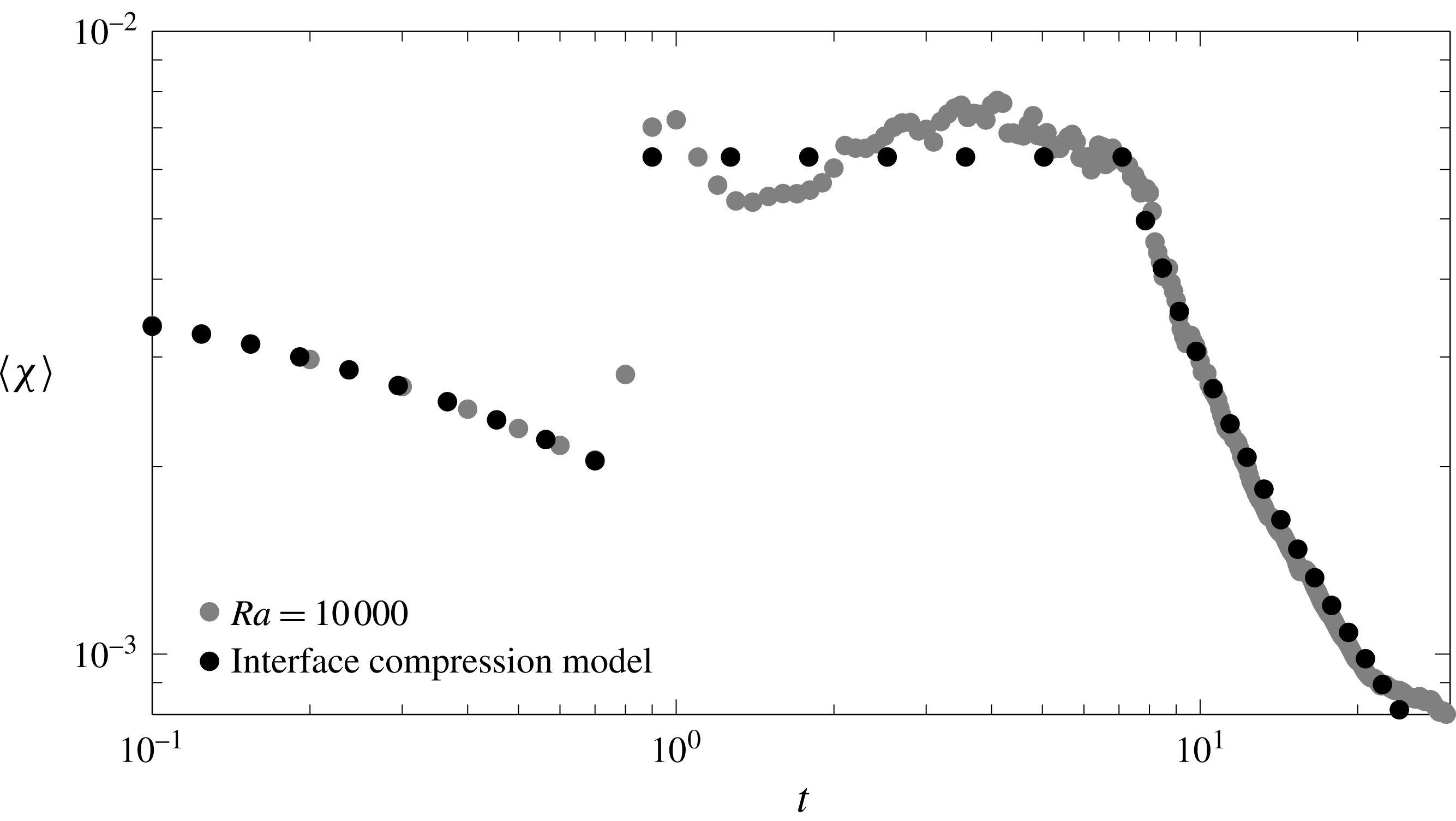
The global scalar dissipation rate (figure 14) shows that there are three main regimes: diffusive, convection dominated and convection shutdown. At the beginning the fluids mix diffusively until the increase of density at the interface creates instabilities that lead to a convection dominated regime. The convection dominated regime is characterized by a constant global scalar dissipation rate and the formation of fingering patterns. As the fluids mix and the concentration difference between the fluids diminishes, convection and mixing slow down.
Evolution with time of the global scalar dissipation rate for the two-fluid system with
 $\mathit{Ra}=10\,000$
for the numerical simulation (grey dots) and the interface compression model (black dots).

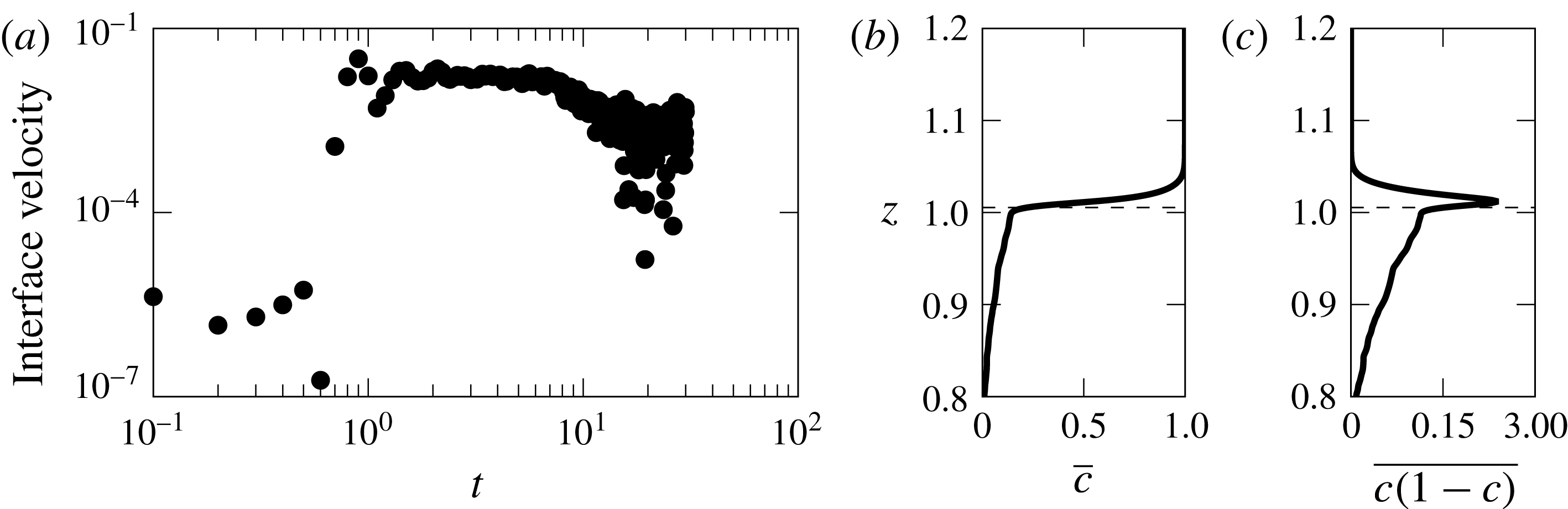
As in the previous problems, mixing is related to the interface and velocity structure evolution. The main difference with the double gyre and the HRL problem is that the interface between the fluids is not at rest as can be seen in the concentration maps in figure 13. As the top fluid dissolves in the bottom fluid the interface moves up. Figure 15(a) shows the velocity of the interface computed from
 $c(1-c)$
as illustrated in panels (b,c). The maximum speed is observed during the convection dominated regime after which the interface velocity decreases.
Interface velocity for the two-fluid system with
 $\mathit{Ra}=10\,000$
(a). Overlines indicate horizontally averaged magnitudes. The interface position is determined as first zero of the derivative of
 $\overline{c(1-c)}$
with respect to
 $z$
after the maximum. This is illustrated in plots (b) and (c) where the
 $\overline{c}$
and
 $\overline{c(1-c)}$
are plotted for
 $t=1.4$
,
 $\mathit{Ra}=10\,000$
. The position of the interface is indicated by the black dashed line.

The compression rate
 $\unicode[STIX]{x1D6FE}$
is given by the net velocity change across the interface as
 $$\begin{eqnarray}\displaystyle & \displaystyle \unicode[STIX]{x1D6FE}=\frac{q_{b}-q_{i}}{s}, & \displaystyle\end{eqnarray}$$
where
 $q_{b}$
is the velocity of the up-welling fluid and
 $q_{i}$
is the interface velocity at the stagnation point. The up-welling fluid moves with a velocity proportional to the difference with respect to the maximum density. For the chosen density law and
 $c_{b}<c_{m}$
,
 $q_{b}$
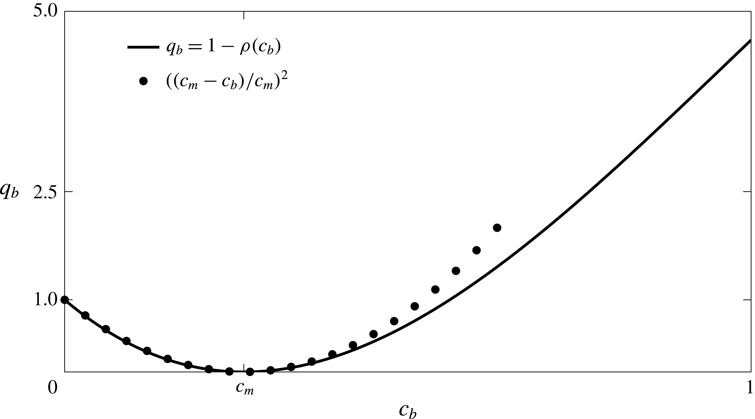
can be approximated by (figure 16)
 $$\begin{eqnarray}\displaystyle & \displaystyle q_{b}(c_{b})=\left(\frac{c_{m}-c_{b}}{c_{m}}\right)^{2}, & \displaystyle\end{eqnarray}$$
where, we recall,
 $c_{b}$
is the average concentration below the interface and
 $c_{m}$
the concentration for which density is maximum.
Buoyancy velocity in the two-fluid system
 $q_{b}=1-\unicode[STIX]{x1D70C}(c_{b})$
(solid line) can be approximated by
 $\left((c_{m}-c_{b})/c_{m}\right)^{2}$
(dots). For the simulations in this study
 $c_{m}=0.26$
.

The velocity of the interface at the stagnation point is proportional to the dissolution flux, therefore
 $$\begin{eqnarray}\displaystyle & \displaystyle q_{i}=\frac{1-c_{b}}{s\,\mathit{Ra}}, & \displaystyle\end{eqnarray}$$
and the compression rate can be written as
 $$\begin{eqnarray}\displaystyle & \displaystyle \unicode[STIX]{x1D6FE}=\frac{1}{s}\left(q_{b}-\frac{1-c_{b}}{s\,\mathit{Ra}}\right). & \displaystyle\end{eqnarray}$$
Then, the steady state solution of (3.1) is approximated by (see Hidalgo et al. Reference Hidalgo, Dentz, Cabeza and Carrera2015)
 $$\begin{eqnarray}\displaystyle & \displaystyle s\approx \frac{2-c_{b}}{(1-c_{b})^{2}\,\mathit{Ra}}. & \displaystyle\end{eqnarray}$$
Equations (6.4) and (6.5) show that the fact that the interface motion leads to a lower compression of the interface and smaller dissolution flux across it than in the HRL problem. The difference in the dissolution flux between fixed and moving interfaces was noted by Hidalgo et al. (Reference Hidalgo, Fe, Cueto-Felgueroso and Juanes2012).
Maximum compression and scalar dissipation rate
 $\unicode[STIX]{x1D712}$
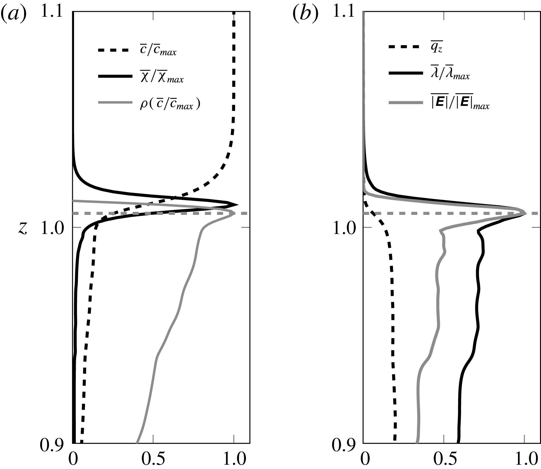
happen at the interface where the maximum strain is also found (figure 13). There is also a high strain on the sides of the fingers, however, their contribution to mixing is small because the concentration difference between the finger centre and the surrounding fluid is low. Moreover, the increasing width of the fingers softens the concentration gradient therefore reducing even more their contribution to the mixing as time passes. The close relation between velocity, mixing and strain is illustrated in figure 17. The maximum strain, indicated by the determinant of the strain tensor and the maximum of its eigenvalues, occurs at the same height as the maximum density. At this position the derivative of
 $q_{z}$
is maximum too. Maximum scalar dissipation rate however, is found a little above that point. This is caused by the nonlinear density law, which makes the interface asymmetric as it is compressed only from the bottom. The interface asymmetry is more severe in the double gyre and the HRL problem because of the fixed boundaries (see figure 3).
Horizontally averaged concentration, scalar dissipation rate and density (a), and vertical component of the velocity, determinant of the strain tensor
 $\unicode[STIX]{x1D640}$
and its maximum eigenvalue
 $\unicode[STIX]{x1D706}$
(b). Some magnitudes are normalized by their maximum value. Maximum mixing is found above the location of maximum compression (horizontal dashed line). Data correspond to the
 $\mathit{Ra}=10\,000$
case for
 $t=1.4$
.

When convection dominates, the up-welling fluid is still the initial one, therefore
 $c_{b}=0$
(figure 18) and
 $q_{b}=1$
. As a result the interface compression is maximum (figure 19). Using (6.5) and (3.6) leads to
 $$\begin{eqnarray}\displaystyle & \displaystyle s_{B}=\frac{2}{\mathit{Ra}} & \displaystyle\end{eqnarray}$$
and
 $$\begin{eqnarray}\displaystyle & \displaystyle \langle \unicode[STIX]{x1D712}\rangle =\frac{\unicode[STIX]{x1D714}_{e}}{4\sqrt{\unicode[STIX]{x03C0}}}, & \displaystyle\end{eqnarray}$$
where
 $\unicode[STIX]{x1D714}_{e}\propto n_{sp}s_{B}$
with
 $n_{sp}$
the number of stagnation points. At the onset of the instability, the fingers distribute according to the wavelength
 $\unicode[STIX]{x1D706}_{c}$
of the most unstable mode. Therefore the
 $n_{sp}$
can be estimated using the results of Riaz et al. (Reference Riaz, Hesse, Tchelepi and Orr2006) as
 $n_{sp}=1/\unicode[STIX]{x1D706}_{c}=(\unicode[STIX]{x1D6FD}_{c}\,\mathit{Ra})/(2\unicode[STIX]{x03C0})$
, which yields
 $\unicode[STIX]{x1D714}_{e}=\unicode[STIX]{x1D6FD}_{c}\unicode[STIX]{x03C0}$
. Finally,
 $$\begin{eqnarray}\displaystyle & \displaystyle \langle \unicode[STIX]{x1D712}\rangle =\frac{2}{\unicode[STIX]{x03C0}^{3/4}}\unicode[STIX]{x1D6FD}_{c}, & \displaystyle\end{eqnarray}$$
which is independent of
 $\mathit{Ra}$
because of the equilibrium between the diffusive interface expansion and the compression exerted by the buoyant fluid. Hidalgo et al. (Reference Hidalgo, Dentz, Cabeza and Carrera2015) obtained
 $\unicode[STIX]{x1D6FD}_{c}=0.018$
from their simulations, which is
 $c_{m}$
times the one reported by Riaz et al. (Reference Riaz, Hesse, Tchelepi and Orr2006) for a linear density law with
 $c_{m}=1$
. Therefore the shape of the density law plays a critical role not only in the location of the maximum compression (figure 17) but also on the value of the scalar dissipation rate during convection.
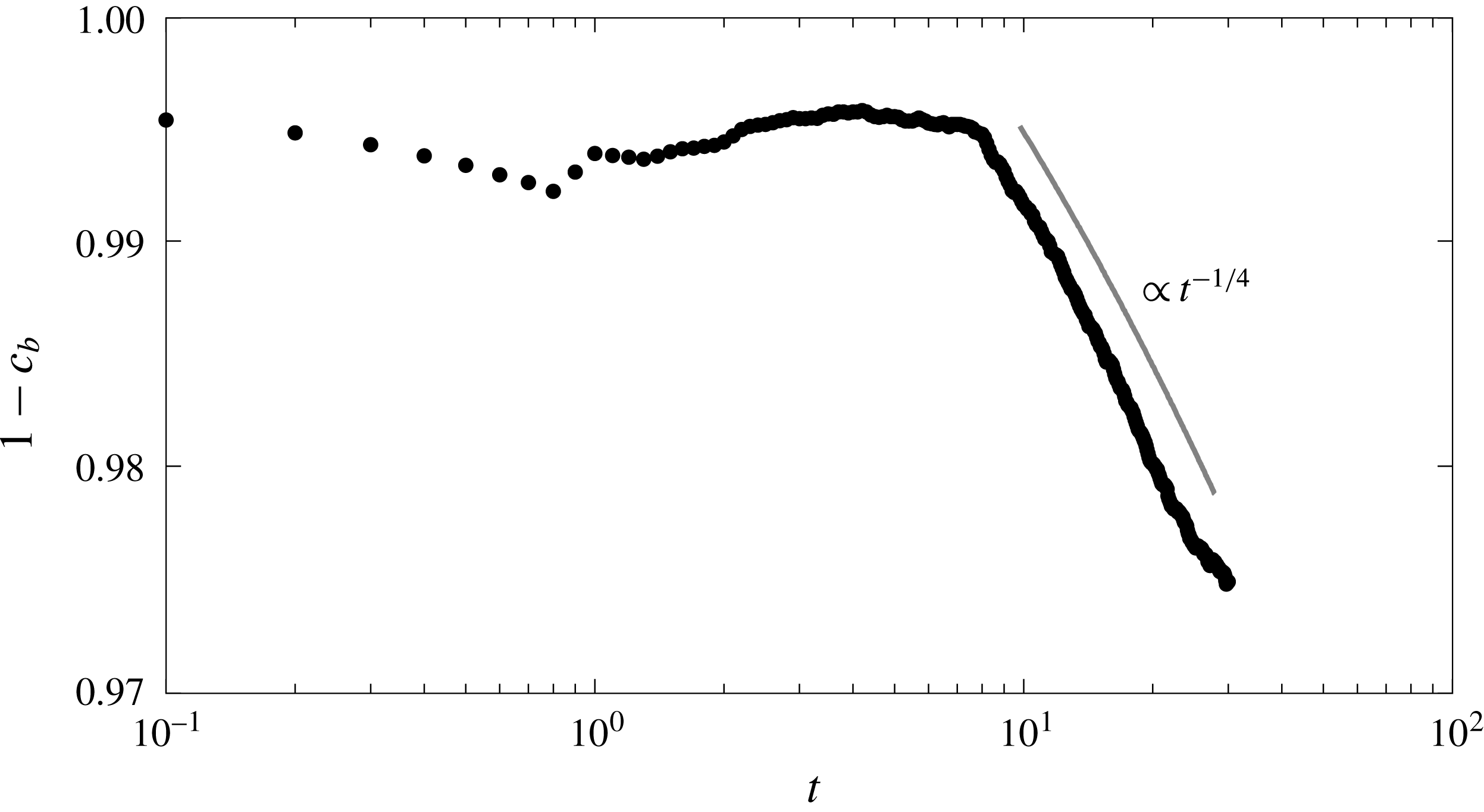
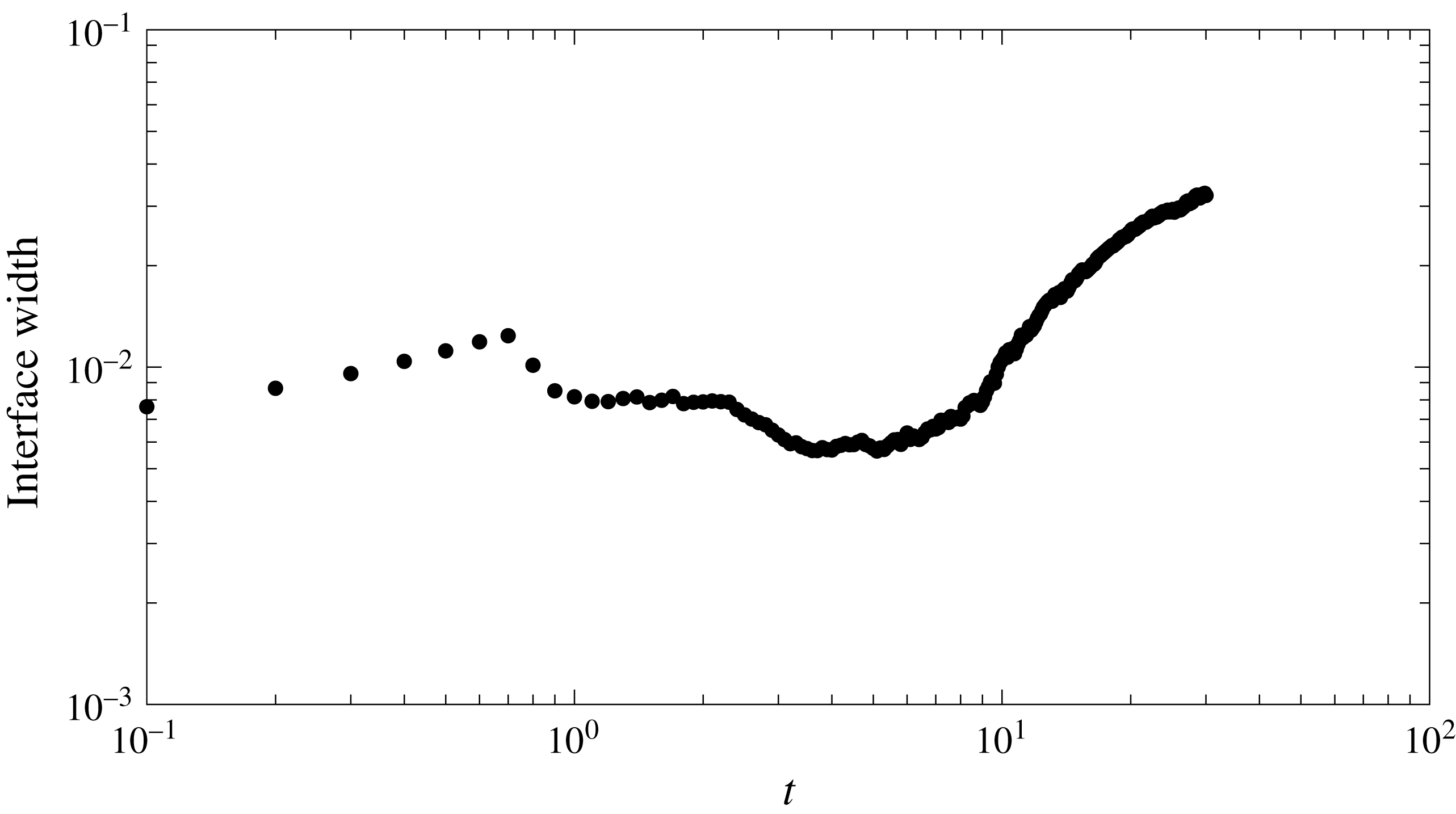
As the concentration of the bottom fluid increases, the interface compression and convection weaken and the interface width grows rapidly as can be seen comparing figures 18 and 19 in which the increase in
 $c_{b}$
happens at the same time the interface width grows. The
 $1-c_{b}\sim t^{-1/4}$
behaviour in figure 18 is in good agreement with the results of Hidalgo et al. (Reference Hidalgo, Dentz, Cabeza and Carrera2015)
 $$\begin{eqnarray}\displaystyle & \displaystyle c_{b}=1-\left[1+2\unicode[STIX]{x1D714}_{e}(t-\unicode[STIX]{x1D70F}_{s})\right]^{-1/4}, & \displaystyle\end{eqnarray}$$
which reproduces well the behaviour of
 $\langle \unicode[STIX]{x1D712}\rangle$
during the convection shutdown regime (see figure 14). In (6.9)
 $\unicode[STIX]{x1D70F}_{s}$
is the time when convection shutdown begins and the effective length behaves as
 $\unicode[STIX]{x1D714}_{e}\propto 0.002\sqrt{\mathit{Ra}}$
reflecting that the Rayleigh number becomes meaningful again when the fingers reach the bottom of the system. From that moment on, the velocity field is again influenced by the domain size and the wide fingers behave similarly to the convection cells of the HRL problem.
Evolution of the average concentration below the interface for the two-fluid system (
 $\mathit{Ra}=10\,000$
). The concentration
 $c_{b}$
is constant during the convection dominated regime and decreases as
 $t^{-1/4}$
during convection shutdown.

Interface width for the two-fluid system (
 $\mathit{Ra}=10\,000$
). The interface width is defined as the square root of the second moment of the horizontal average of
 $c(1-c)$
. This value follows the expected temporal evolution but overestimates the value of the interface width because of the influence of the fingers (see figure 15).

As the regimes succeed each other, the structure of the velocity field changes (figure 13). The maximum velocity is found during the convection dominated regime and decreases as convection shuts down. The velocity autocorrelation
 $\text{ACF}_{|\boldsymbol{q}|}$
(figure 13
d) reflects the horizontal structure of the fingering pattern with a decreasing number of local maxima as fingers coarsen. During the convection dominated regime the velocity and its autocorrelation are similar to the high
 $\mathit{Ra}$
HRL problem (compare
 $\mathit{Ra}=10\,000$
in figure 8 to
 $t=3.5$
in figure 13). During convection shutdown after the fingers hit the bottom of the domain, the velocity structure resembles that of the low
 $\mathit{Ra}$
HRL problem because the fingering patterns are similar to elongated convection cells (compare
 $\mathit{Ra}=750,1000$
in figure 8 to
 $t=30$
in figure 13).
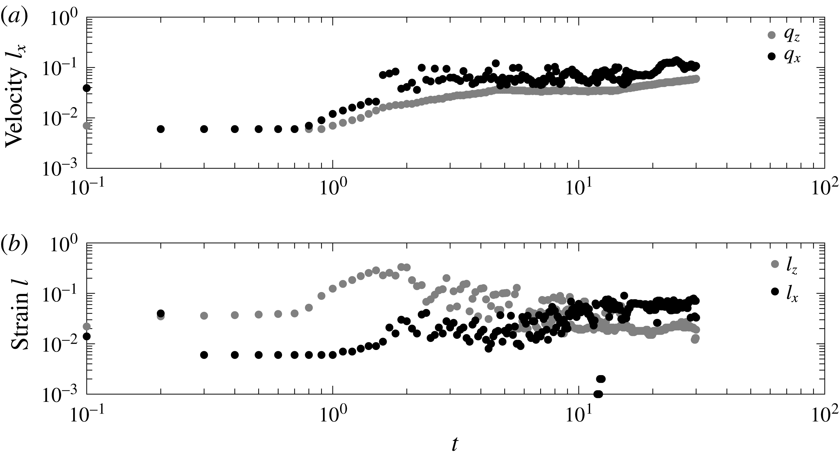
The velocity and strain correlation lengths also evolve during the three regimes (figure 20). The velocity correlation length in both directions is minimum before the onset of convection after which the maximum velocity is found. Then, the velocity correlation length reflects the creation of the fingering pattern. While the correlation length of
 $q_{z}$
grows and stabilizes around a constant value, the correlation length of
 $q_{x}$
continues growing as new fingers form and merge. A similar behaviour is observed for the correlation length of the strain. Its correlation length in horizontal direction follows that of the horizontal velocity. In the vertical direction, however, the maximum correlation length is found after the onset of convection. This is caused by the growing fingers along which there is a high strain. At late times it decreases as the strain along the fingers becomes weaker.
Evolution with time of the velocity correlation length in the horizontal direction for both components of the velocity (a) and strain correlation length in both directions (b) for the two-fluid system with
 $\mathit{Ra}=10\,000$
.

6.3 Mixing state
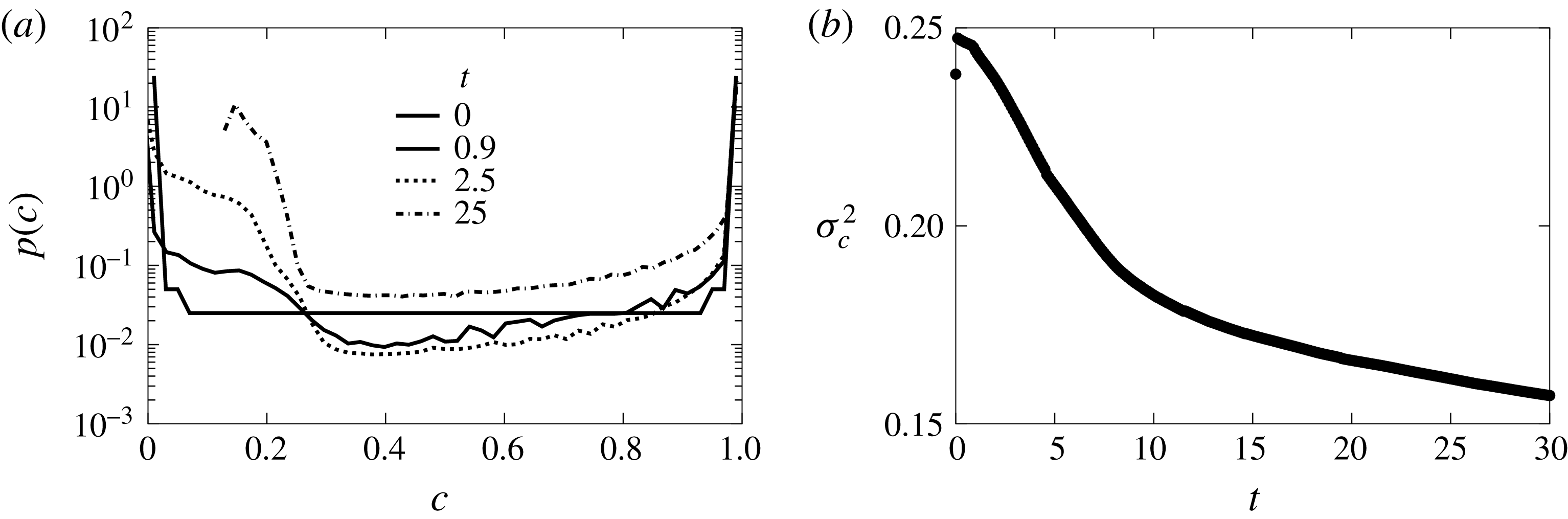
The mixing state of the system also changes with the different regimes. In the beginning the system mixes slowly by diffusion and the concentration p.d.f. has two distinct peaks at the extreme concentrations (figure 21
a). When convection takes over, the peak around the low concentration shifts as a consequence of the mixing created by the fingers. The peak around maximum concentration is widen by the effect of diffusion. Eventually diffusion will take the system to a well-mixed state with uniform 0.5 concentration because the fluids occupied the same volume initially. However, there is an intermediate state of duration proportional to
 $Ra$
characterized by a skewed concentration p.d.f. displaying high probabilities around the concentration of the initial top fluid (
 $c=1$
) and a peak near
 $c_{m}$
as shown in figure 21(a) for
 $t=25$
.
In the two-fluid system there are no boundary dissolution fluxes, therefore,
 $\langle \unicode[STIX]{x1D712}\rangle$
is proportional to the time derivative of the concentration variance. Figure 21(b) shows how the system homogenization evolves in accordance with
 $\langle \unicode[STIX]{x1D712}\rangle$
. Initially, the mixing state is given by the initial conditions. During the onset of the instabilities
 $\unicode[STIX]{x1D70E}_{c}^{2}$
increases. However, it reduces as soon as they are fully developed. This shows that the chaotic convection that creates the fingering structures is an efficient mixing mechanism. As convection shuts down, the bottom fluid mean concentration approaches
 $c_{m}$
for which density is maximum and the density stratification approaches to a stable configuration. Then, convection weakens and the fingers merge and become wider, which makes the gradients of concentration at the interface and below smaller. In this regime the mixing efficiency decreases as well as the speed at which the system evolves towards the well-mixed state.
(a) Concentration p.d.f. and (b) its variance for different times and
 $\mathit{Ra}=10\,000$
.

7 Conclusions
We have studied mixing in porous media under unstable flow conditions using an interface compression model that is able to reproduce the observed behaviour of the global scalar dissipation rate
 $\langle \unicode[STIX]{x1D712}\rangle$
(equivalent to the Nusselt number). The model, introduced through the analysis of a problem with a synthetic double-gyre velocity field, links the dissolution fluxes to the interface width. The width of the interface is modified by the velocity field, whose characteristics are related to the kind of instabilities and the concentration evolution.
The Horton–Rogers–Lapwood problem was used to study a Rayleigh–Bénard instability in which the fluid interface is immobile. The system displays two regimes. First, it organizes itself into convection cells as in the double gyre. During this regime the velocity field is not independent of the domain size and the compression rate
 $\unicode[STIX]{x1D6FE}$
is independent of diffusion, which leads to
 $\langle \unicode[STIX]{x1D712}\rangle \propto \mathit{Ra}^{-1/2}$
. Then, above
 $\mathit{Ra}_{c}$
, the convection cells turn into columnar plumes. The velocity autocorrelation decreases abruptly and the system’s size becomes irrelevant so that
 $\unicode[STIX]{x1D6FE}$
is of the order of
 $1/s_{B}$
, therefore related to diffusion, and
 $\langle \unicode[STIX]{x1D712}\rangle \propto \mathit{Ra}^{0}$
.
The case in which the interface is mobile was analysed using a Rayleigh–Taylor instability in which the unstable density stratification was achieved by the mixture of two fluids with a non-monotonic density law. The system experiences three regimes. A diffusive regime in which the interface between the fluids grows. Then, a convection dominated regime after the onset of the instabilities in which
 $\langle \unicode[STIX]{x1D712}\rangle$
is independent of
 $\mathit{Ra}$
. This behaviour is similar to the high
 $\mathit{Ra}$
HRL problem. The domain size does not affect the buoyancy fluxes and the interface width is controlled by a compression rate linked to diffusion. Finally, a convection shutdown regime in which the system slowly approaches to a stable density stratification as the fluids mix. This regime is characterized by a temporal dependency of
 $\langle \unicode[STIX]{x1D712}\rangle$
. The system then behaves as finite and the correlation length of the velocity grows.
The interface compression model and the analysis of the velocity field revealed that the scaling of
 $\langle \unicode[STIX]{x1D712}\rangle$
is linked to the system’s size experienced by the velocity field. When the velocity field and concentration patterns are constrained by the domain boundaries,
 $\langle \unicode[STIX]{x1D712}\rangle \propto \mathit{Ra}^{-1/2}$
. However, when the structure of the velocity field breaks because of the strong convection, the size of the domain becomes unimportant and
 $\langle \unicode[STIX]{x1D712}\rangle$
independent of
 $\mathit{Ra}$
.
We have shown that the global scalar dissipation
 $\langle \unicode[STIX]{x1D712}\rangle$
is controlled by the dynamics of the fluid interface around the velocity field stagnation points. It is therefore expected that the stagnation points play an central role in the location and magnitude of mixing induced chemical reactions. The reaction hot spots will be preferentially found near the locations where maximum dissolution (and maximum local scalar dissipation rate) takes place. The fingering and columnar patterns contribute much less to
 $\langle \unicode[STIX]{x1D712}\rangle$
. However they are essential for the mixing state of the system.
The mixing state of the system also depends on the nature of the instabilities. The variance of concentration decreases by the mixing of the convection patterns and increases because of the fluxes through the boundaries. The double-gyre and HRL problems reach a steady mixing state in which both effects equilibrate and the variance of the concentration remains constant. In both cases convection makes the system more homogeneous. For low
 $\mathit{Ra}$
, the steady state is achieved earlier and the dissolution fluxes are bigger because they are proportional to
 $\mathit{Ra}^{-1/2}$
. For high
 $\mathit{Ra}$
, the system is better mixed and displays a narrower concentration p.d.f. but it takes more time to arrive to that state. The Rayleigh–Taylor instability lacks boundary fluxes. The evolution of the mixing state is governed by the scalar dissipation rate. During the period in which convection dominates mixing is maximum as well as the dissolution fluxes. As convection ceases the efficiency of the system to mix itself decreases. Therefore, the better mixed the system is, the lower the dissolution fluxes. This suggest that a certain level of segregation might be desirable to maintain chemical reactions and fluxes through the boundary. Contrary to intuition, the best mixing state, i.e. lower variance of concentration, is attained for high
 $\mathit{Ra}$
. That is a reduction in diffusion favours the homogenization of the concentration. This homogenization is achieved by the stirring created by the instability patterns.
Acknowledgements
J.J.H. and M.D. acknowledge the support of the European Research Council through the project MHetScale (FP7-IDEAS-ERC-617511). J.J.H. acknowledges the support of the Spanish Ministry of Economy and Competitiveness through the project Mec-MAT (CGL2016-80022-R).