1 Introduction
The experiments of Matas, Morris & Guazzelli (Reference Matas, Morris and Guazzelli2003) have shed light on the non-monotonic effect of particles in laminar–turbulent flow transition, depending on the particle-to-pipe size ratio and on the suspension volumetric concentration. A small amount of neutrally buoyant finite-size particles allowed for the sustaining of the turbulent state and decreased the transition threshold significantly. Almost a decade later, particle-resolved numerical simulations provided some evidence that, at moderate concentrations, particles have a significant impact on the unsteady nature of the flow, enhancing the transverse turbulent stress components and modifying the flow rotational structures (Loisel et al.
Reference Loisel, Abbas, Masbernat and Climent2013; Yu et al.
Reference Yu, Wu, Shao and Lin2013; Lashgari, Picano & Brandt Reference Lashgari, Picano and Brandt2015). The effect of particles on the transition of Couette flow is not yet well characterized. Recent experiments from Majji, Banerjee & Morris (Reference Majji, Banerjee and Morris2018) have shown that particles do not have a significant impact on the transition path in Taylor-Couette flow, if the particle concentration is low and the particle size is relatively small compared to the Couette gap. With larger particles (eight times smaller than the Couette gap), Linares-Guerrero, Hunt & Zenit (Reference Linares-Guerrero, Hunt and Zenit2017) have shown that particles do not change the transition threshold of a cylindrical turbulent Couette flow at
 $10\,\%$
volumetric concentration. Consistent with this finding, flow statistics performed on moderately concentrated turbulent plane Couette flow (slightly above the transition threshold), have revealed that there is no significant difference between single- and two-phase flows at equivalent effective Reynolds number (Wang, Abbas & Climent Reference Wang, Abbas and Climent2017).
If the size of the particles is large enough compared to the size of energetic eddies in a turbulent flow, the local flow streamlines are significantly modified (as would not be the case for pointwise particles). The rigid body constraints from finite-size particles influence the turbulent kinetic energy budget in two competing ways: they add perturbations that increase shear production of turbulence and simultaneously increase viscous dissipation (Qureshi et al. Reference Qureshi, Bourgoin, Baudet, Cartellier and Gagne2007; Bellani et al. Reference Bellani, Byron, Collignon, Meyer and Variano2012). The perturbations induced by the particles depend on their locations: their magnitude increases with the local flow strain rate. The spatial distribution of neutrally buoyant particles depends on the flow configuration (turbulent Couette or channel flow). Indeed, in addition to the turbulent dispersion that particles undergo, they experience a lift force due to finite flow inertia at the particle scale. This lift force is normal to the walls, and its orientation depends on the flow configuration. Therefore, particles are preferentially located either in the active region, i.e. near the walls in pressure-driven channel flow (Loisel et al. Reference Loisel, Abbas, Masbernat and Climent2013), or in the inactive region, i.e. away from the walls in Couette flow (Wang et al. Reference Wang, Abbas and Climent2017).
Even though the stability in Couette and channel single-phase flows is different, they share, at high Reynolds numbers, some common turbulence features in the near-wall regions. In the inner region of a boundary layer, the turbulent motion consists of an active part and an inactive part based on Townsend (Reference Townsend1980). Near the walls, the active motion contains eddies with a streamwise characteristic length of the order of
 $1000$
wall units in highly turbulent flows that constitute the essential contribution to the Reynolds shear stress (
 $-\overline{u^{\prime }v^{\prime }}$
) (throughout the study,
 $u$
,
 $v$
and
 $w$
denote the velocity components in the flow, shear and vorticity directions
 $x$
,
 $y$
and
 $z$
respectively). Statistical properties of the flow stress in the active region are universal functions of the wall shear stress
 $\unicode[STIX]{x1D70F}_{w}$
and the wall-normal position
 $y$
, whereas the inactive motion gives no correlation between
 $u^{\prime }$
and
 $v^{\prime }$
and it is mainly related to the flow geometry (Bradshaw Reference Bradshaw1967; Panton Reference Panton2001; Jiménez Reference Jiménez2011; Tuerke & Jiménez Reference Tuerke and Jiménez2013). The essential difference in the flow configurations is due to the mean velocity (
 $\overline{u}$
) profile which is anti-symmetric (respectively symmetric) in plane Couette (respectively pressure-driven) flow with respect to the midplane. The production term (
 $-\overline{u^{\prime }v^{\prime }}\,\text{d}\overline{u}/\text{d}y$
) in the turbulent kinetic energy equation has different roles according to the flow configuration. In Couette flow, the fluid is pumped away from one wall to the other, extracting energy from the mean flow, leading to the enhancement of turbulent structures (Papavassiliou & Hanratty Reference Papavassiliou and Hanratty1997). However, in pressure-driven channel flow, the shear layers are divided into two regions and the production is of opposite sign in each channel half, making the turbulent structures relatively independent of each wall.
The temporal and spatial development of wall turbulence consists of a self-sustained process, namely the near-wall regeneration cycle (located in the vicinity of the no-slip boundary condition
 $20<y^{+}<60$
: see Waleffe Reference Waleffe1997). During this complete cycle, coherent large-scale streaks and alternating staggered rotating vortices sustain each other, altogether having an impact on the wall friction. This cycle has been demonstrated to be independent of the outer layer: it can survive without any input from the core flow. Indeed Jiménez & Pinelli (Reference Jiménez and Pinelli1999) carried out simulations after removing all the fluctuations from the velocity field above
 $y^{+}=60$
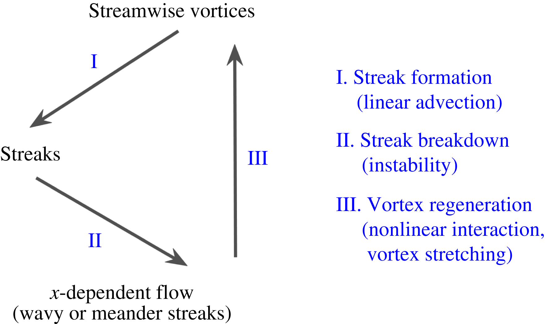
(in a channel flow), and after hundreds of time units, they observed an almost unchanged turbulent flow compared to the original one. The regeneration cycle consists of three sequential sub-processes sketched in figure 1: streak formation, streak breakdown and streamwise vortex regeneration. The streaks are generated by a linear process, the so-called lift-up effect, whereas the following two processes are the result of nonlinear interactions.
Sketch of the regeneration cycle sub-steps.

In order to understand how particles affect the flow turbulence and the transition from one regime to another, we are concerned in this paper with their impact on the regeneration cycle. Klinkenberg et al. (Reference Klinkenberg, Sardina, De Lange and Brandt2013) have shown that inertial pointwise particles modify the transition to turbulence not by altering the lift-up effect but rather by modifying the dynamics of the oblique waves necessary for the streak regeneration and breakdown. In this work, we consider the effect of neutrally buoyant finite-size particles on the regeneration cycle, in turbulent flows slightly above the transition limit of single-phase flows (Reynolds number equal to 500 for Couette and 2600 for channel flows). Numerical simulations are performed in a domain (so-called miniunit) which contains one set of coherent structures sufficient to sustain the flow turbulence. The size of this miniunit is different for each flow and follows the findings of Jiménez & Moin (Reference Jiménez and Moin1991) and Hamilton, Kim & Waleffe (Reference Hamilton, Kim and Waleffe1995). The coupling between the fluid motion and the particle dynamics is taken into account using the force coupling method (Climent & Maxey Reference Climent, Maxey, Feuillebois and Sellier2009). Neutrally buoyant particles
 $20$
times smaller than the Couette gap or channel height are considered here at moderate volumetric concentration from
 $1$
up to
 $10\,\%$
.
The paper is organized as follows. Section 2 summarizes the numerical configurations in both single- and two-phase flows. In § 3, we show how particles affect the laminar–turbulent transition by using specific initial conditions for each flow configuration. Then, we discuss the effect of particles on the flow energy modulation in § 4 and on the different stages of the regeneration cycle in § 5. Both analogies and divergences for Couette and pressure-driven flows are discussed throughout the paper before the conclusion.
2 Suspension flow configurations
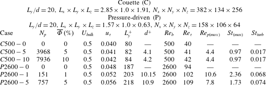
The coupling of fluid flow and particle dynamics follows the force coupling method (FCM), as described in Wang et al. (Reference Wang, Abbas and Climent2017). The validation tests were carefully detailed. The method is valid to study suspension Couette or pressure-driven channel flows, with particle Reynolds numbers (
 $Re_{p}$
is defined in table 1) up to
 $10$
and particle volume fraction less than
 $20\,\%$
.
Parameters of the numerical simulations. The Reynolds number
 $Re_{b}\equiv U_{bulk}h/\unicode[STIX]{x1D708}$
for Couette flow and
 $Re_{b}\equiv Q/\unicode[STIX]{x1D708}$
for channel flow.
 $h=L_{y}/2$
is half of the Couette gap or channel height. In channel flow, the flow rate per unit depth is
 $Q=4U_{bulk}L_{y}/3$
.
 $U_{bulk}$
is the velocity of the moving walls in Couette flow whereas it is half the central velocity that the channel flow would have if the flow was laminar. The Reynolds number based on the friction velocity and on the channel half-width is
 $Re_{\unicode[STIX]{x1D70F}}\equiv u_{\unicode[STIX]{x1D70F}}h/\unicode[STIX]{x1D708}$
. The particle Reynolds number
 $Re_{p}\equiv \unicode[STIX]{x1D6E4}a^{2}/\unicode[STIX]{x1D708}$
based on local shear rate
 $\unicode[STIX]{x1D6E4}=|\text{d}\overline{u}/\text{d}y|$
, and the Stokes number
 $St\equiv 2\unicode[STIX]{x1D70C}_{p}/(9\unicode[STIX]{x1D70C}_{f})Re_{p}$
are low near the Couette and channel centres and they are maximum near the walls where the shear rate is the highest. The maximum particle Reynolds and Stokes numbers are based on the shear rate calculated at one particle diameter away from the walls.

Couette flow was driven by two walls moving at equal and opposite velocities. Pressure-driven channel flow was generated by imposing a global pressure drop in the streamwise direction, that is tuned over time in order to maintain constant flow rate. In both flow configurations,
 $x$
and
 $z$
are respectively the streamwise and spanwise flow directions, with periodic boundary conditions (the so-called homogeneous directions), while
 $y$
stands for the wall-normal or velocity gradient direction. Turbulent flow simulations were performed using a so-called ‘miniunit’ configuration, which is the minimal geometric domain that is sufficient to accommodate the self-sustained flow structures for single-phase turbulence, while allowing reasonable time for the computation of suspension flows with finite-size particles. The minimal simulation domain (different in each flow configuration) was carefully examined in Couette flow configuration by Hamilton et al. (Reference Hamilton, Kim and Waleffe1995) and pressure-driven flow by Jiménez & Moin (Reference Jiménez and Moin1991). In both cases, the spanwise length is larger than 100 wall units, which corresponds to the spanwise characteristic spacing between two coherent structures. The length and velocity in wall units are
 $y^{+}\equiv yu_{\unicode[STIX]{x1D70F}}/\unicode[STIX]{x1D708}$
, and
 $u^{+}\equiv u/u_{\unicode[STIX]{x1D70F}}$
, where
 $u_{\unicode[STIX]{x1D70F}}=\sqrt{\unicode[STIX]{x1D70F}_{w}/\unicode[STIX]{x1D70C}}$
is the friction velocity based on the wall shear stress and fluid density.
Table 1 contains a summary of all the parameters selected for this study. Throughout the paper, we denote
 $C$
for plane Couette and
 $P$
for pressure-driven channel flows. The size ratio between the Couette gap or channel height and the particle diameter is
 $L_{y}/d=20$
in most cases. Particles experience turbulent fluctuations, and their inertia can be characterized by the dimensionless Stokes number
 $St_{turb}=\unicode[STIX]{x1D70F}_{p}^{+}/\unicode[STIX]{x1D70F}_{f}^{+}$
, where
 $\unicode[STIX]{x1D70F}_{p}^{+}$
is the particle relaxation time scale in response to the turbulent flow forcing, whose characteristic time scale is
 $\unicode[STIX]{x1D70F}_{f}^{+}$
. The latter is considered here as the ratio between the characteristic size of the large-scale streamwise vortices
 $L_{y}^{+}$
in Couette flow or
 $L_{y}^{+}/2$
in channel flow, and the characteristic velocity fluctuation scale
 $\max (v^{\prime +},w^{\prime +})$
in the flow cross-section. The ability of the FCM to capture accurately the particle response to flow fluctuations was tested in Wang et al. (Reference Wang, Abbas and Climent2017), where the motion of a rigid particle submitted to an external oscillating force in a still fluid was considered. The numerical solution of the particle motion was in a good agreement with the theoretical prediction when the ratio of the particle radius to the developed Stokes layer thickness
 $\unicode[STIX]{x1D6FF}^{2}\equiv \unicode[STIX]{x1D714}a^{2}/\unicode[STIX]{x1D708}$
was less than
 $2$
(
 $\unicode[STIX]{x1D714}$
being the oscillation frequency of the external forcing). This ratio is directly related to the particle Reynolds and Stokes numbers, i.e.
 $\unicode[STIX]{x1D6FF}^{2}=9\unicode[STIX]{x03C0}St_{turb}/(\unicode[STIX]{x1D70C}_{p}/\unicode[STIX]{x1D70C}_{f}+1/2)$
. In the simulations considered for this work, with neutrally buoyant particles,
 $\unicode[STIX]{x1D6FF}^{2}$
is always below
 $0.5$
in Couette flow and
 $1.4$
in pressure-driven flow.
Table 1 contains also the Stokes number based on the local shear which achieves its maximum value near the channel or near the walls in Couette flow, where the shear rate is the highest. It is nearly 1 in Couette and 2.4 in channel flow. Note that the results of simulations in Couette flow with
 $1<St<4~(4<d^{+}<8)$
reported in Wang et al. (Reference Wang, Abbas and Climent2017) were similar to those obtained in the present paper at
 $St\approx 1~(d^{+}\approx 4)$
. For both flow configurations, the effect of particles on the statistics were formed at an effective Reynolds number
 $40\,\%$
–
 $50\,\%$
higher than the corresponding critical Reynolds number (estimated from figure 2).
3 Particle effect on the transition
A theoretical analysis of flow stability in the presence of freely moving finite-size particles is actually impossible, from a mathematical point of view. For this reason we determined the transition threshold from an engineering point of view, by considering a fully developed turbulent flow experiencing successive reductions of the Reynolds number down to a limit where the flow becomes eventually laminar. Every time the Reynolds number was decreased, the simulation was run for longer than
 $500$
time units. Transition of single-phase flow was observed at
 $Re_{c\_C}\sim 320$
for Couette and at
 $Re_{c\_P}\sim 2200$
for pressure-driven flows. It should be kept in mind that, first, the value of the critical Reynolds number depends on the simulation domain because periodic boundary conditions influence interactions between large-scale vortices. Second, relaminarization is a process that may occur randomly. Therefore the determination of a ‘rigorous’ laminar–turbulent transition threshold (which is not the main scope of the present paper) would require a large number of simulations to form statistics. Instead, an indicative threshold is determined in order to assess the impact of the particle presence on the flow features, and to evaluate qualitatively an eventual transition delay or enhancement.
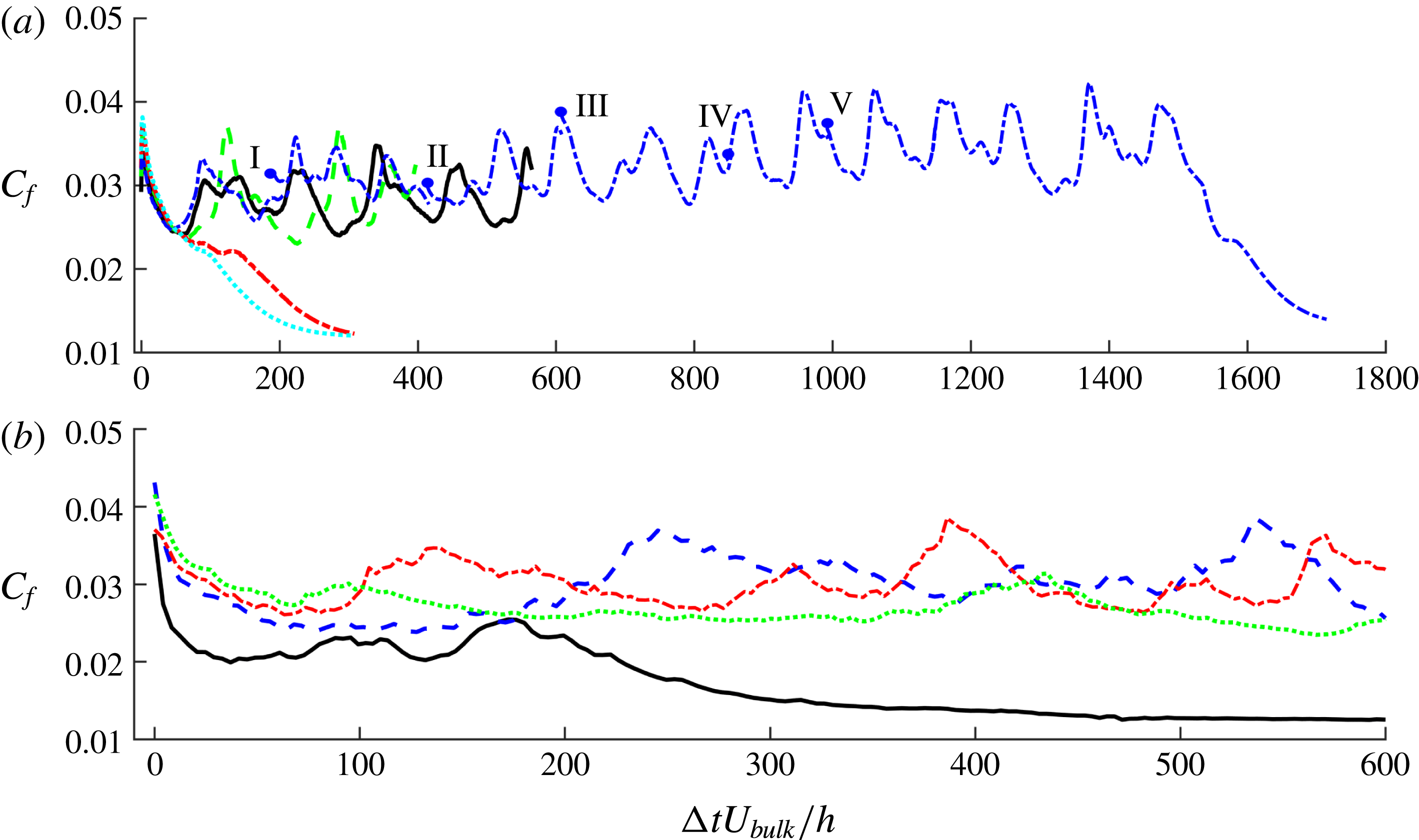
Effect of neutrally buoyant particles on the laminar–turbulent transition threshold, as depicted from the temporal evolution of
 $C_{f}$
, after decreasing
 $Re_{b}$
in (a) Couette flow and (b) pressure-driven flow. The initial flow configuration of the Couette (respectively channel) flow is taken from a fully turbulent simulation at
 $Re_{b}=500$
(respectively 2300). (a) ——
 $Re_{b}=500$
,
 $\unicode[STIX]{x1D6F7}=5\,\%$
; – – – (green)
 $Re_{b}=470$
,
 $\unicode[STIX]{x1D6F7}=10\,\%$
; – - – - (red)
 $Re_{b}=455$
,
 $\unicode[STIX]{x1D6F7}=10\,\%$
;
 $\cdots \cdots$
(cyan)
 $Re_{b}=440$
,
 $\unicode[STIX]{x1D6F7}=10\,\%$
; – - – - (blue)
 $Re_{b}=455$
–345,
 $\unicode[STIX]{x1D6F7}=5\,\%$
and
 $I$
to
 $V$
corresponding to
 $Re_{b}=455$
,
 $415$
,
 $390$
,
 $365$
and
 $355$
. (b) ——
 $Re_{b}=2000$
,
 $\unicode[STIX]{x1D6F7}=1\,\%$
; – – – (blue)
 $Re_{b}=2000$
,
 $\unicode[STIX]{x1D6F7}=5\,\%$
; – - – - (red)
 $Re_{b}=1700$
,
 $\unicode[STIX]{x1D6F7}=5\,\%$
;
 $\cdots \cdots$
(green)
 $Re_{b}=1500$
,
 $\unicode[STIX]{x1D6F7}=5\,\%$
.

In the range of suspension flow parameters investigated (particle size and volumetric concentration), particles are expected to decrease significantly the laminar–turbulent transition threshold in pressure-driven flow based on the experiments of Matas et al. (Reference Matas, Morris and Guazzelli2003), in opposition to Couette flow where particles seem not to affect the flow stability (see our previous study in Wang et al.
Reference Wang, Abbas and Climent2017). The wall friction coefficient
 $C_{f}$
(summed on both walls) was considered as an indicator of the current flow regime,
 $C_{f}=2\overline{\unicode[STIX]{x1D70F}}_{w}/(\unicode[STIX]{x1D70C}U_{bulk}^{2})$
for Couette flow and
 $2\overline{\unicode[STIX]{x1D70F}}_{w}/(\unicode[STIX]{x1D70C}(Q/L_{y})^{2})$
for pressure-driven flow. The initial flow configurations were chosen from the single-phase flow simulations at
 $Re_{b}=500$
for Couette and
 $Re_{b}=2300$
for channel flow. The particles were then randomly seeded in the simulation domain, at different volumetric concentrations (
 $\unicode[STIX]{x1D6F7}=5$
or
 $10\,\%$
in Couette and
 $\unicode[STIX]{x1D6F7}=1$
or
 $5\,\%$
in channel flow). The two-phase flow simulations were carried out for several hundreds of time units (typically more than
 $300$
), before the Reynolds number was decreased in order to evaluate the transition threshold. The evolution in time of the wall friction coefficient of the suspension flow is shown in figure 2 for different cases, after the Reynolds number was abruptly decreased.
In Couette flow, the Reynolds number was decreased from
 $500$
separately to
 $470$
,
 $455$
or
 $440$
. At
 $\unicode[STIX]{x1D6F7}=10\,\%$
, the flow became laminar for the two simulations at
 $Re_{b}=455$
and
 $440$
. At
 $\unicode[STIX]{x1D6F7}=5\,\%$
, the flow remained turbulent at
 $Re_{b}=455$
. When the Reynolds number was progressively decreased as follows:
 $455\rightarrow 415\rightarrow 390\rightarrow 365\rightarrow 355$
, the transition took place only around
 $Re_{c}\approx 355$
. This critical Reynolds number is calculated using the pure fluid viscosity. The effective Reynolds number based on the suspension viscosity is lower if additional viscous dissipation introduced by the rigid particles is accounted for, due to an increase of the flow viscosity
 $\unicode[STIX]{x1D708}_{eff}=\unicode[STIX]{x1D708}\unicode[STIX]{x1D702}(\unicode[STIX]{x1D6F7},Re)$
, with
 $\unicode[STIX]{x1D702}(\unicode[STIX]{x1D6F7},Re)>1$
. There are some possibilities to predict
 $\unicode[STIX]{x1D702}(\unicode[STIX]{x1D6F7},0)$
from Eilers’ fit (Stickel & Powell Reference Stickel and Powell2005) and the correction at finite Reynolds number
 $\unicode[STIX]{x1D702}(\unicode[STIX]{x1D6F7},Re)$
and low concentrations (see for example Subramanian et al.
Reference Subramanian, Koch, Zhang and Yang2011). The simulations with FCM give access to the increase of the suspension viscosity induced by the particles through the second-order term of the multipole expansion, also called a stresslet (for the definition, see Wang et al.
Reference Wang, Abbas and Climent2017). This leads to a critical Reynolds number for the suspension flow
 $Re_{c,s}\approx 312$
for
 $\unicode[STIX]{x1D6F7}=5\,\%$
which is very close to the value of single-phase flow
 $Re_{c\_C}$
. The main conclusion of this test is that in a Couette flow with moderate particle concentration, the particles act mainly as a source of energy dissipation in the flow, and that they do not change significantly the transition threshold if the suspension viscosity was taken into account in the Reynolds number definition.
In pressure-driven flow, the initial flow configuration was selected at
 $Re_{b}=2300$
. Particles were randomly seeded at concentrations of
 $1\,\%$
or
 $5\,\%$
. A small concentration of finite-size particles is enough to decrease the transition threshold (see Matas et al.
Reference Matas, Morris and Guazzelli2003; Loisel et al.
Reference Loisel, Abbas, Masbernat and Climent2013; Yu et al.
Reference Yu, Wu, Shao and Lin2013; Lashgari et al.
Reference Lashgari, Picano and Brandt2015), keeping in mind that at low to moderate concentration, the threshold decreases when the concentration is increased, in contrast to Couette flow. Figure 2(b) shows the temporal evolution of
 $C_{f}$
after particles were seeded and the Reynolds number was decreased from
 $2300$
to
 $2000$
. For
 $\unicode[STIX]{x1D6F7}=1\,\%$
, the flow is fully laminar at
 $Re_{b}=2000$
. However for
 $\unicode[STIX]{x1D6F7}=5\,\%$
, a stable two-sided turbulent flow is sustained at
 $Re_{b}=2000$
while Jiménez & Moin (Reference Jiménez and Moin1991) observed that in the miniunit turbulent flow exists only near one wall in a single-phase flow, even at higher Reynolds number (
 $Re_{b}=2667$
). Decreasing
 $Re_{b}$
from
 $2300$
to
 $1700$
and then to
 $1500$
, the flow becomes laminar at
 $Re_{c}=1500$
(which corresponds to
 $Re_{c,s}=1315$
based on Eilers’ fit whereas
 $Re_{c,s}=1150$
based on 5
c). A significant drop of the transition threshold (
 $Re_{c\_P}\sim 2200$
for single-phase flow) is observed although the effective viscosity has increased.
3.1 Influence of particles on the flow stability
As will be further discussed in § 4.1, particles tend to accumulate in the large-scale vortex regions in Couette flow and in low-speed streak regions in channel flow. In order to understand how particles enhance or reduce the flow stability from their preferential spatial distribution, we carried out some simulations with specific flow configurations.
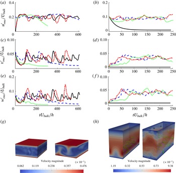
Particle effect on flow stability. (a,c,e,g) Couette flow starting from a fully turbulent regime. The turbulent state is stable under a single-phase condition; even when the streamwise velocity perturbations are suppressed, the flow recovers its fully turbulent nature. Adding particles damps the velocity fluctuations and makes the flow laminar. ——
 $Re_{b}=430$
, single-phase flow removes
 $u^{\prime }$
; – – –
 $Re_{b}=430$
,
 $\unicode[STIX]{x1D6F7}=5\,\%$
and
 $L_{y}/d=10$
; – - – -
 $Re_{b}=455$
, single-phase flow removes
 $u^{\prime }$
;
 $\cdots \cdots$
 $Re_{b}=455$
,
 $\unicode[STIX]{x1D6F7}=10\,\%$
and
 $L_{y}/d=20$
. (b,d,f,g) Channel flow starting with a flow distribution according to (3.1) where an artificial streak is initially imposed. The single-phase flow tends towards the laminar state at
 $Re_{b}=2600$
which is above the laminar–turbulent transition. Adding a small number of particles in the flow triggers the transition to turbulence. —— single-phase flow; – – –
 $\unicode[STIX]{x1D6F7}=0.5\,\%$
and
 $L_{y}/d=16$
; – - – -
 $\unicode[STIX]{x1D6F7}=0.75\,\%$
and
 $L_{y}/d=16$
;
 $\cdots \cdots$
 $\unicode[STIX]{x1D6F7}=0.5\,\%$
and
 $L_{y}/d=20$
.

The first test was done in Couette flow and it was inspired by the study of Hamilton et al. (Reference Hamilton, Kim and Waleffe1995). When the streamwise velocity perturbations were removed, while the linear streamwise velocity profile and streamwise vortices were maintained from a fully turbulent simulation, the authors observed that the flow evolved again to the fully turbulent regime. In a similar way, we considered for the initial configuration a snapshot from a steady single-phase turbulent Couette flow simulation at
 $Re_{b}=500$
where the large-scale
 $x$
-independent streak is maximum (from
 $M(0,\unicode[STIX]{x1D6FD})$
defined in (4.1)). We removed the streaks, and abruptly decreased the Reynolds number to
 $455$
and
 $430$
in two separate simulations.
The temporal evolution of root-mean-square (r.m.s.) velocity fluctuations shown in figure 3(a,c,e) as well as the mean velocity profile (not shown here) suggest that, despite the initial destabilization, the flow recovers its fully turbulent features after
 $200$
time units. Figure 3(g) shows the contours of velocity magnitude for single-phase flow; the left figure is taken at
 $t=0$
after removing
 $u^{\prime }$
and its evolution after
 $500$
time units can be seen in the right figure. The flow field plotted after nearly five regeneration cycles cannot be distinguished from the initial fully turbulent flow. Therefore the streamwise vortices, that were initially maintained, were strong enough to generate streaks through the lift-up effect and resume the regeneration cycle.
The main effect of the presence of particles in the Couette flow is stabilizing in nature. When we added small particles (
 $L_{y}/d=20$
) at
 $\unicode[STIX]{x1D6F7}=10\,\%$
and decreased the Reynolds number down to
 $455$
, without removing the streamwise velocity perturbations, the flow became laminar. Adding larger particles (
 $L_{y}/d=10$
) at
 $\unicode[STIX]{x1D6F7}=5\,\%$
and decreasing the Reynolds number to
 $430$
, the flow velocity fluctuations were significantly damped, and the flow became laminar after staying quasi-turbulent for around six regeneration cycles. These observations suggest that the particles were mainly enhancing dissipation in the flow.
The test of flow stability for the channel flow configuration has been done using an artificial finite-amplitude low-speed streak that was supplemented to a mean flow profile corresponding to wall-bounded turbulence. We used the same base flow as Schoppa & Hussain (Reference Schoppa and Hussain2002), who studied the streak transient growth mechanism in a two-dimensional streak configuration. The base flow is
 $$\begin{eqnarray}u(y,z)=U_{0}(y)+(\unicode[STIX]{x0394}u/2)\cos (\unicode[STIX]{x1D6FD}_{s}z)g(y)\end{eqnarray}$$
in the streamwise direction, and
 $v=w=0$
in the wall-normal and spanwise directions.
 $U_{0}(y)$
is the mean velocity and
 $g(y)$
is an amplitude function which satisfies the no-slip condition at
 $y=0$
and localizes the streak velocity defect at a single wall. A ‘single-sided’ turbulent mean velocity profile is imposed, analogous to that observed in minimal channel turbulence (Jiménez & Moin Reference Jiménez and Moin1991), with a parabolic profile
 $U_{lam}$
in the laminar top half of the channel, and a turbulent Reichardt profile
 $U_{turb}$
that respects the near-wall turbulence statistics, in the bottom half:
 $$\begin{eqnarray}U_{0}(y)=\left\{\begin{array}{@{}l@{}}\displaystyle U_{lam}=U_{c}[1-((y/h)-1)^{2}],\quad y_{m}\leqslant y\leqslant 2h,\\ \displaystyle U_{turb}=u_{\ast }\left[2.5\ln (1+0.4y/\unicode[STIX]{x1D6FF})+7.8\left(1-\text{e}^{(-y/11\unicode[STIX]{x1D6FF})}-\frac{y}{11\unicode[STIX]{x1D6FF}}\text{e}^{(-y/3\unicode[STIX]{x1D6FF})}\right)\right],\\ \hspace{30.00005pt}0\leqslant y<y_{m}.\end{array}\right.\end{eqnarray}$$
The friction velocity
 $u_{\ast }=\sqrt{\unicode[STIX]{x1D70F}_{w}/\unicode[STIX]{x1D70C}}$
and viscous length scale
 $\unicode[STIX]{x1D6FF}=\unicode[STIX]{x1D708}/u_{\ast }$
are calculated using a wall shear stress estimated from Dean’s empirical correlation (
 $C_{f}\equiv 2\unicode[STIX]{x1D70F}_{w}/\unicode[STIX]{x1D70C}\overline{u}^{2}=0.073Re_{b}^{-0.25}$
) in a fully turbulent channel flow. For a given flow rate
 $Q$
, this leads the friction velocity to be
 $u_{\ast }=Q\sqrt{0.0365(Q/\unicode[STIX]{x1D708})^{-0.25}}/(2h)$
. The two profiles
 $U_{turb}$
and
 $U_{lam}$
are matched at a wall-normal distance
 $y_{m}$
in the turbulent half, with
 $y_{m}$
and
 $U_{c}$
determined so that the mean flow velocity and vorticity are continuous at the matching point, i.e.
 $U_{lam}(y_{m})=U_{turb}(y_{m})$
and
 $\text{d}U_{lam}/\text{d}y\mid _{y=y_{m}}=\text{d}U_{turb}/\text{d}y\mid _{y=y_{m}}$
. Consequently, at
 $Re=Q/\unicode[STIX]{x1D708}=2600$
,
 $y_{m}=0.918h$
and
 $U_{c}=1.2Q/(2h)$
.
The function
 $g(y)\sim y\cdot \text{e}^{-\unicode[STIX]{x1D702}y^{2}}$
accounts for the streak velocity defect, and has been normalized to unity with
 $\unicode[STIX]{x1D702}$
specified such that the streak velocity defect
 $\unicode[STIX]{x0394}u$
and normal vorticity
 $\unicode[STIX]{x1D6FA}_{y}\mid _{max}=\unicode[STIX]{x1D6FD}_{s}\unicode[STIX]{x0394}u/2$
exhibit a plateau in the range
 $y^{+}=10-30$
, consistent with the observed lifted streaks and
 $\unicode[STIX]{x1D714}_{y,rms}$
statistics. Note that the amplitude function
 $g(y)$
in (3.1) determines the strength of the local streak upper bound
 $u(y)$
shear layer (e.g. local maximum of
 $\unicode[STIX]{x2202}u/\unicode[STIX]{x2202}y$
) residing on the crest of the lifted streak. Instability growth rates for the dominant sinuous modes are found to be relatively insensitive to the strength of this shear layer and hence to the amplitude function
 $g(y)$
. The value
 $\unicode[STIX]{x1D702}=20$
was used similarly to Schoppa & Hussain (Reference Schoppa and Hussain2002). The streak spanwise wavenumber
 $\unicode[STIX]{x1D6FD}_{s}$
in (3.1) is chosen as
 $2\unicode[STIX]{x03C0}/\unicode[STIX]{x1D6FD}_{s}^{+}=100$
, corresponding to the well-accepted average spanwise spacing of adjacent low-speed streaks observed in many experimental and numerical studies.
Figure 3(h), left, shows the velocity magnitude contours of the flow according to (3.1). Schoppa & Hussain (Reference Schoppa and Hussain2002) found that this single-phase flow is stable and the energy of the artificial streaky perturbation will vanish in time due to viscous dissipation. A spanwise perturbation, following a sinuous profile in the flow direction, is necessary to trigger the growth in time of the perturbation. In the absence of such spanwise initial coherent motion, figure 3(b,d,f) confirms that the perturbation (3.1) is damped over time when the Reynolds number is equal to
 $2600$
(above the transition threshold).
Unlike the Couette flow test, the particles in this particular channel flow were not seeded throughout the entire domain. Of course this would lead the flow to undergo the transition to turbulence. Instead, we seeded a small number of particles only in the low-speed artificial streak region (
 $u(y,z)/U_{bulk}\leqslant 1.5$
) keeping the flow Reynolds number
 $Re_{b}=2600$
. Two different local concentrations (particles-to-streak volume) were considered (
 $\unicode[STIX]{x1D6F7}=0.5$
and
 $0.75\,\%$
for the case of
 $L_{y}/d=16$
and
 $\unicode[STIX]{x1D6F7}=0.5\,\%$
for the case of
 $L_{y}/d=20$
). In all cases, the particle presence triggered the transition to turbulence (this can be evidenced by the level of the r.m.s. velocity signals), and the particles were found after
 ${\sim}100$
time units spread all over the simulation domain. Figure 3(h), right, shows the contours of velocity magnitude for suspension flow in the case of
 $L_{y}/d=16$
with
 $\unicode[STIX]{x1D6F7}=0.75\,\%$
after
 $250$
time units. We can observe a quasi-fully turbulent state at
 $Re_{b}=2600$
(instead of the one-sided wall turbulence observed in single-phase flow noted by Jiménez & Moin Reference Jiménez and Moin1991).
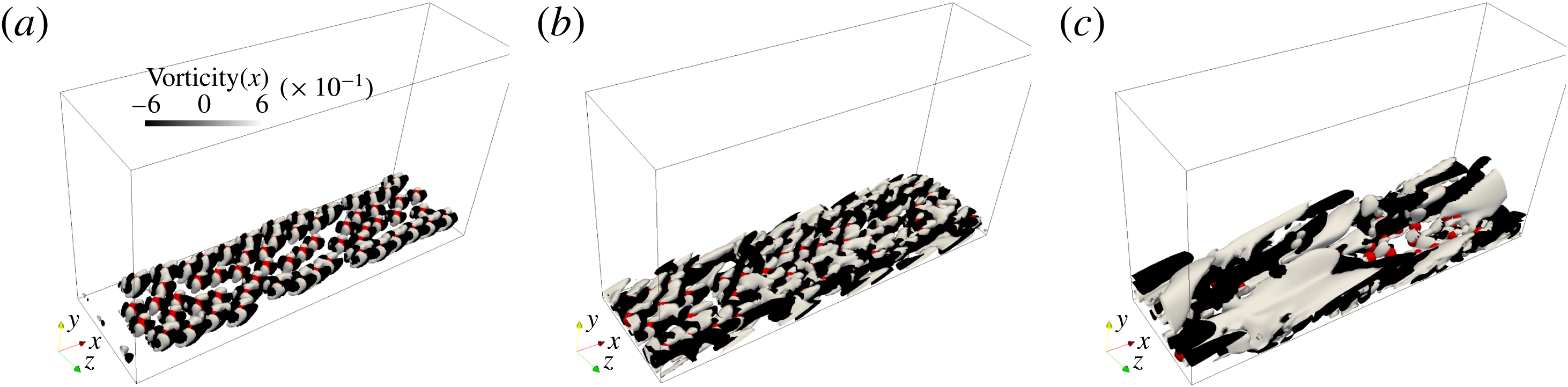
Flow vorticity induced by a layer of particles seeded in the plane
 $y/d=0.8$
(near the wall) in the same flow configuration as 3(h). The total volume concentration is
 $\unicode[STIX]{x1D6F7}=0.5\,\%$
, and the size ratio
 $L_{y}/d=16$
is used. The snapshots are taken at three time instants
 $t=0.2$
,
 $2.7$
and
 $29.5$
(scaled by
 $h/U_{bulk}$
) which correspond to
 $t^{+}=2$
,
 $27$
and
 $295$
(scaled by
 $\unicode[STIX]{x1D708}/u_{\unicode[STIX]{x1D70F}}^{2}$
).

The influence of the particles on the transition is also illustrated in figure 4, showing the temporal evolution of the streamwise vorticity generated by the particles. The initial condition is equivalent to figure 3(h), except that
 $60$
particles were initially seeded in a plane parallel to the wall (instead of being located in the artificial streak). At the first instants (figure 4
a), streamwise vorticity is generated around finite-size particles due to the secondary flows occurring at finite
 $Re_{p}$
. As time goes on and particles move, this streamwise vorticity is stretched in the streamwise direction, as in figure 4(b). Furthermore, these structures are tilted due to the mean shear through the streamwise vorticity generation term
 $-(\unicode[STIX]{x2202}w/\unicode[STIX]{x2202}x)(\unicode[STIX]{x2202}u/\unicode[STIX]{x2202}y)$
(explained in § 5) which is large near the wall. They further interact with each other to form larger-scale streamwise vortical structures, as shown in figure 4(c). Clearly the generated vortical structures are comparable to the near-wall vorticity layers induced by large-scale vortices, which are the essential ingredients of the regeneration cycle for channel flow.
4 Modulation of the turbulent flow energy
In this section, we show that particles modulate the flow energy in a channel more strongly than in Couette flow. The statistics are formed in physical and Fourier space in order to study the regeneration cycle. In physical space, profiles are obtained by averaging the data over the two homogeneous (streamwise and spanwise) directions. As for the spectral analysis, it is performed either close to the wall or across the whole gap between the walls. In addition, a modal analysis of the flow fluctuating energy is considered, and will be shortly introduced here. The Fourier decomposition of the energy, as introduced by Hamilton et al. (Reference Hamilton, Kim and Waleffe1995) over two periodic directions, streamwise and spanwise, is written as follows:
 $$\begin{eqnarray}\displaystyle & & \displaystyle M(k_{x}=m\unicode[STIX]{x1D6FC},k_{z}=n\unicode[STIX]{x1D6FD})\nonumber\\ \displaystyle & & \displaystyle \quad \equiv \,\left\{\int _{Y_{1}}^{Y_{2}}[|\widehat{u^{\prime }}|^{2}(m\unicode[STIX]{x1D6FC},y,n\unicode[STIX]{x1D6FD})+|\widehat{v^{\prime }}|^{2}(m\unicode[STIX]{x1D6FC},y,n\unicode[STIX]{x1D6FD})+|\widehat{w^{\prime }}|^{2}(m\unicode[STIX]{x1D6FC},y,n\unicode[STIX]{x1D6FD})]\,\text{d}y\right\}^{1/2},\end{eqnarray}$$
where
 $Y_{1}$
and
 $Y_{2}$
stand for the integration bounds in the wall-normal direction.
 $(\unicode[STIX]{x1D6FC},\unicode[STIX]{x1D6FD})$
are the fundamental wavenumbers in the streamwise and spanwise directions defined as
 $(2\unicode[STIX]{x03C0}/L_{x},2\unicode[STIX]{x03C0}/L_{z})$
, and
 $m$
and
 $n$
are integers. The intensity of any turbulent structure can be represented by one mode
 $(m\unicode[STIX]{x1D6FC},n\unicode[STIX]{x1D6FD})$
.
Since flow modulation is partly related to the particle spatial distribution, the latter will be discussed first.
4.1 Particle dispersion
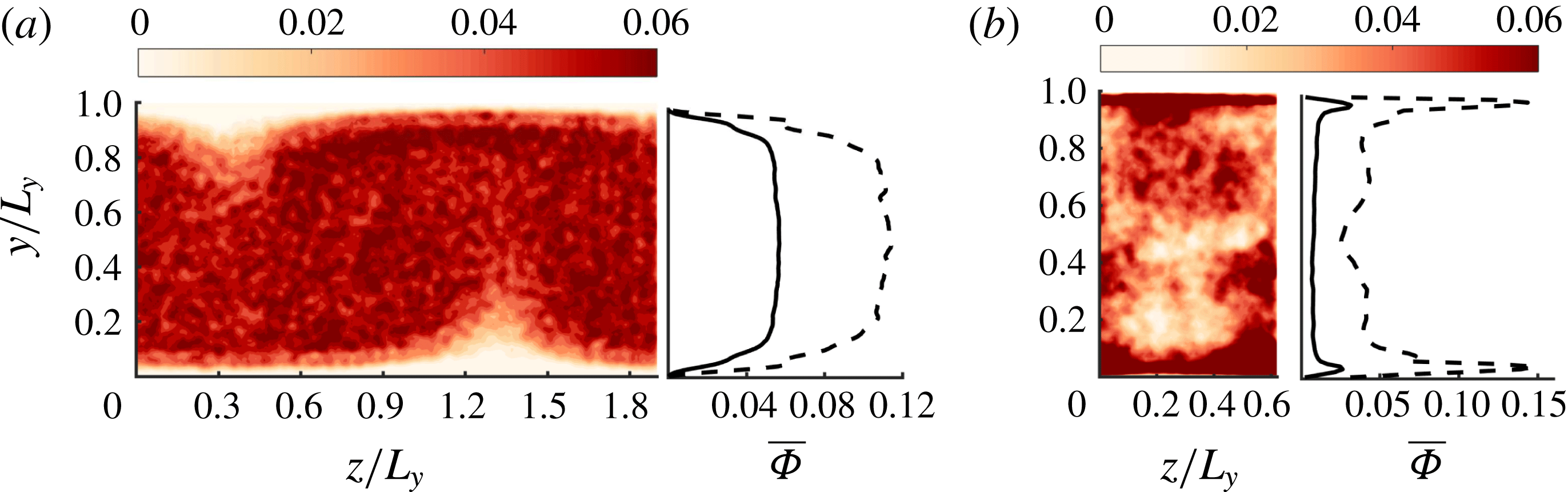
Figure 5(a,b) shows the average particle distribution over the cross-sectional plane. The contours of concentration are averaged over
 $80$
time units (
 $h/U_{bulk}$
) whereas the wall-normal concentration profiles were averaged over
 $500$
time units. The maximum concentration is located in the core region of the Couette flow, whereas two peaks can be observed near the walls of the channel flow. The average concentration profiles are the result of a balance between the lift force on the finite-size particles, the hydrodynamic repulsion from the wall and the shear-induced turbulent diffusion. To be more specific, in laminar plane Couette flow (linear flow), a finite-size neutrally buoyant particle exhibits a (rotational and translational) slip with respect to the local flow field. The pressure is larger on the side of the particle closer to the wall, and thereby the particle is pushed away from the wall (Ho & Leal Reference Ho and Leal1974). When the velocity profile is not linear (quadratic for Poiseuille flow), the particle experiences an inertia-induced lift force (Asmolov Reference Asmolov1999), resulting from its perturbation (as a rigid body) to the quadratic velocity profile (see a review paper by Matas, Morris & Guazzelli Reference Matas, Morris and Guazzelli2004). This force is oriented towards the wall. This is known as the Segré–Silberberg or pinch-off effect. The particle also experiences a hydrodynamic viscous repulsion when it is very close to the wall. The balance between these two opposite forces leads to equilibrium positions (in laminar channel flow) that depend on the particle Reynolds number, and yield segregation of a suspension in channel flow (see Matas et al.
Reference Matas, Morris and Guazzelli2004; Loisel et al.
Reference Loisel, Abbas, Masbernat and Climent2015)
(a,b) Particle distribution in the cross-section (
 $y{-}z$
plane) of Couette
 $C500-5$
and pressure-driven
 $P2600-5$
flows respectively. The concentration contours are averaged in the streamwise direction, over 80 time units. The corresponding concentration profiles, averaged over 500 time units, are also shown for ——
 $C500-5$
, – – –
 $C500-10$
in (a), and ——
 $P2600-1$
, – – –
 $P2600-5$
in (b).

(a,b) Particle distribution in a plane parallel to the wall (
 $x{-}z$
plane) in Couette
 $C500-5$
and pressure-driven
 $P2600-5$
flows respectively. The concentration contours taken at
 $y/L_{y}=0.2$
are averaged over
 $80$
time units. The isolines show
 $u^{\prime }/U_{bulk}$
in the
 $x$
–
 $z$
plane, where dashed lines stand for negative and solid lines for positive values, the interval being
 $0.04$
in (a) and
 $0.03$
in (b). The spanwise variation of the fluid (black) and particle (dashed blue) fluctuation velocity
 $u^{\prime }/U_{bulk}$
averaged in the streamwise direction is also plotted on the right sides of (a,b), separately. (c,d) The streamwise velocity profiles of —— fluid phase (black line), particle phase (blue dashed line) and slip (red dot-dashed line) velocities (defined as the fluid velocity with the particulate phase velocity subtracted). The cross symbols indicate the velocity profile for the single-phase flow.

The instantaneous spatial distribution of particles is shown together with the streamwise velocity fluctuation contours in the
 $x$
–
 $z$
plane (figure 6
a,b). These figures show a strong correlation between the particle spatial distribution and the flow coherent structures. In Couette flow, particles are pulled away from the walls by turbulent ejection and towards the wall by the sweep events. On average, they are more present in the sweep and core regions in Couette flow. In channel flow, the particles are accumulated in the ejection region, near the wall. This can be understood as follows: the inertial lift force drives the particles to be preferentially located near the walls, where high- and low-speed flow regions are encountered. Sweeps are regions of spanwise divergence near the wall which drive the particles to leave the high-speed (sweep) region towards the low-speed (ejection) region. When a particle is dragged away from the wall by an ejection event, there is an opposite hydrodynamic contribution that reduces this effect. Lubrication force acting on a particle moving away from a flat wall is attractive to the wall (and decreases when the particle is far from the wall). The resulting particle migration should depend on the particle size and the distance from the wall. Thus the outward wall-normal flow in the ejection region is most probably insufficient to pull the neutrally buoyant particles, leading to particle accumulation in that region.
The profiles of the fluid, particle and slip velocity (fluid velocity minus particulate-phase velocity) are shown in figure 6(c,d). Also, the spanwise variation of the slip velocity is shown in this figure. The velocity of the particulate phase is always smaller than the local fluid velocity in both Couette and pressure-driven flow configurations (on average particles are lagging the flow), especially near the walls, in both flow configurations.
4.2 Quadrant analysis of velocity r.m.s.
The coherent structures are the major contributors to the Reynolds shear stress. They play an essential role in the active motion of wall turbulence. According to the quadrant analysis, the flow fluctuations can be divided into
 $Q1(u^{\prime }>0,v^{\prime }>0)$
,
 $Q2(u^{\prime }<0,v^{\prime }>0)$
,
 $Q3(u^{\prime }<0,v^{\prime }<0)$
and
 $Q4(u^{\prime }>0,v^{\prime }<0)$
.
 $Q2$
and
 $Q4$
correspond to the ejection and sweep events respectively,
 $Q1$
and
 $Q3$
contain the outward and inward interactions respectively (see a recent review on quadrant analysis by Wallace Reference Wallace2016). We give details of the impact of particles on the different Reynolds stress components, by considering separately the different contributions according to the quadrant analysis.
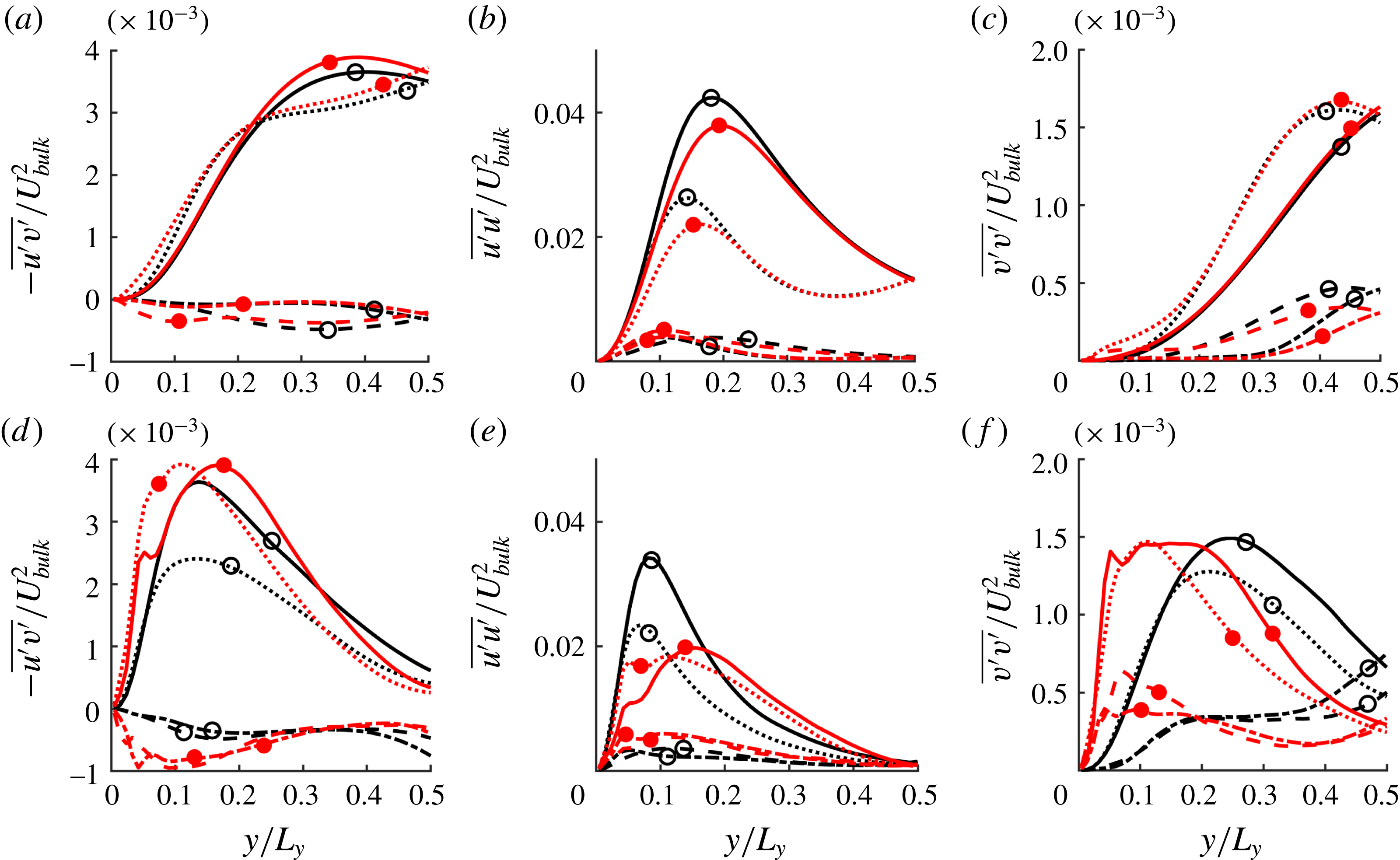
Velocity r.m.s. of single- and two-phase flows in different quadrants: (a–c) Couette flow; (d–f) channel flow. The line style denotes the quadrant: – – –
 $Q1$
, ——
 $Q2$
, – - – -
 $Q3$
,
 $\cdots \cdots$
 $Q4$
. The symbols refer to the flow concentration: open circles for single-phase flow and filled circles for
 $\unicode[STIX]{x1D719}=5\,\%$
. (a,d), (b,e), (c,f)
 $-\overline{u^{\prime }v^{\prime }}$
,
 $\overline{u^{\prime }u^{\prime }}$
and
 $\overline{v^{\prime }v^{\prime }}$
, respectively.

The r.m.s. velocity profiles are displayed in figure 7, according to the quadrant analysis, for both single-phase and suspension flow at
 $\unicode[STIX]{x1D6F7}=5\,\%$
. The Reynolds stress components are not significantly influenced when particles are present in Couette flow at
 $5\,\%$
(figure 7
a–c). However, in channel flow, profiles of the Reynolds shear stress (figure 7
d) reveal that the particles enhance significantly the shear stress in the sweep (
 $Q4$
) part of the logarithmic region, where
 $Q2$
and
 $Q4$
events are dominant. The streamwise Reynolds stress is decreased by the particles, especially in the ejection regions, whereas the wall-normal Reynolds stress is increased in both sweep and ejection regions. The peaks of the profiles are also closer to the wall.
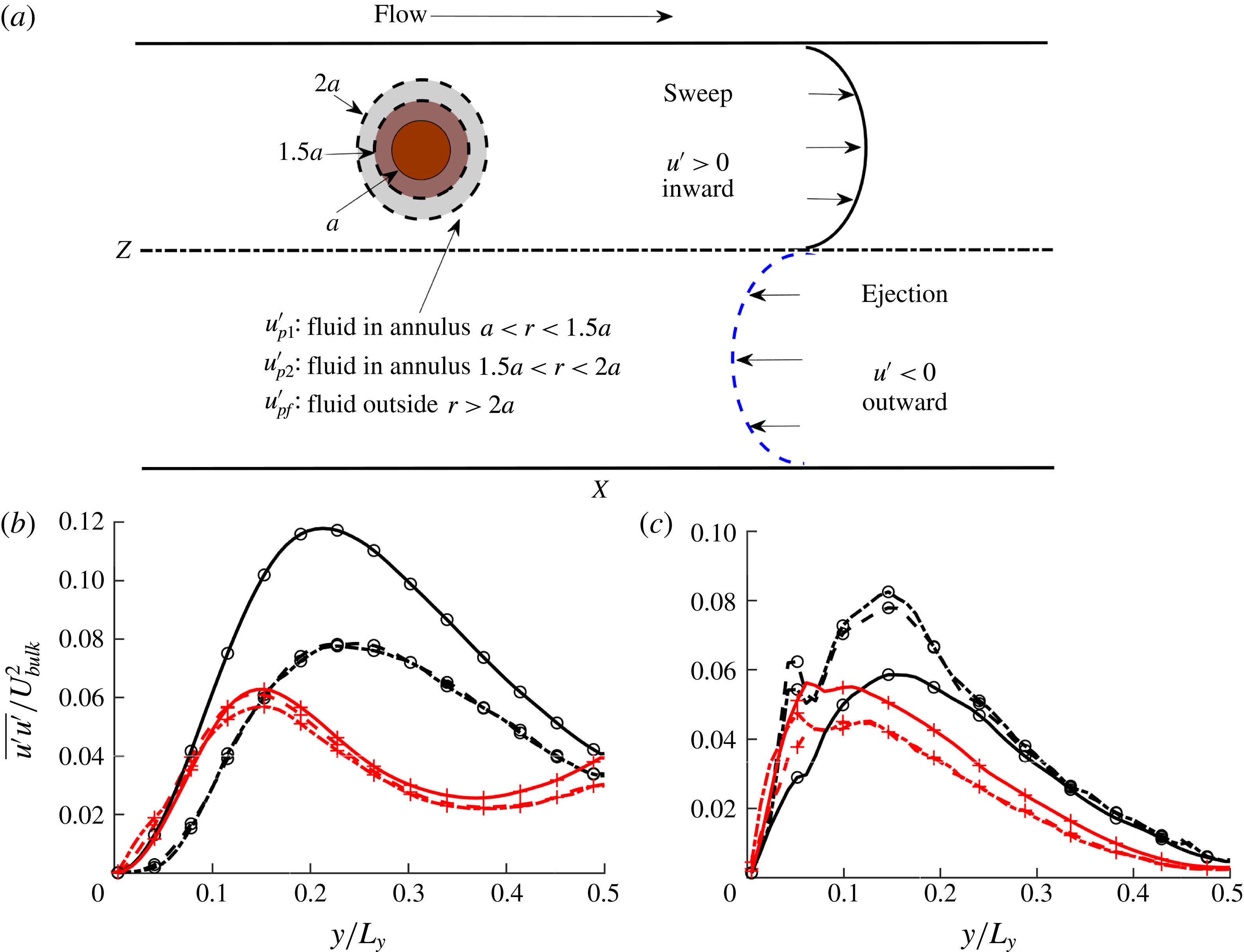
As sketched in (a), the velocity r.m.s. of single- and two-phase flows in
 $Q2$
and
 $Q4$
are split into contributions near the particle surface (
 $\overline{u_{p1}^{\prime }u_{p1}^{\prime }}$
within
 $a<r<1.5a$
using dot-dashed lines and
 $\overline{u_{p2}^{\prime }u_{p2}^{\prime }}$
within
 $1.5a<r<2a$
using dashed lines), and far from the particle surface (
 $\overline{u_{f}^{\prime }u_{f}^{\prime }}$
within
 $r>2a$
using solid lines). The profiles in (b,c) are from Couette and channel flow respectively. Here the circles correspond to the ejection and the plus signs to the sweep events.

These turbulent stress modifications suggest a more isotropic turbulence in a channel flow compared to a single-phase flow, in agreement with previous numerical results obtained using the total profiles of the Reynolds stress components (see Shao, Wu & Yu Reference Shao, Wu and Yu2012; Loisel et al.
Reference Loisel, Abbas, Masbernat and Climent2013; Picano, Breugem & Brandt Reference Picano, Breugem and Brandt2015; Fornari et al.
Reference Fornari, Formenti, Picano and Brandt2016; Yu, Vinkovic & Buffat Reference Yu, Vinkovic and Buffat2016), the transfer between different directions being promoted by the Reynolds shear stress. Particular attention is drawn here to the reduction of the streamwise Reynolds stress component. Fornari et al. (Reference Fornari, Formenti, Picano and Brandt2016) related this observation to the fluid squeezed between the layer of particles near the wall and the wall itself. Shao et al. (Reference Shao, Wu and Yu2012) associated this with the weakening intensity of the large-scale streamwise vortices, a phenomenon that is not observed in Fourier space, as shown later in figure 10(d) and figure 9(e,f). In an attempt to understand why the streamwise Reynolds stress is decreased, we calculated the velocity fluctuations in the fluid far from and close to the particles separately, as sketched in figure 8(a).
 $\overline{u_{f}^{\prime }u_{f}^{\prime }}$
is averaged within the fluid region located at
 $r>2a$
relative to each particle centre.
 $\overline{u_{p1}^{\prime }u_{p1}^{\prime }}$
and
 $\overline{u_{p2}^{\prime }u_{p2}^{\prime }}$
are averaged in the neighbourhood of the particles
 $a<r<1.5a$
and
 $1.5a<r<2a$
, respectively. The profiles of
 $\overline{u_{f}^{\prime }u_{f}^{\prime }}$
,
 $\overline{u_{p1}^{\prime }u_{p1}^{\prime }}$
and
 $\overline{u_{p2}^{\prime }u_{p2}^{\prime }}$
are plotted in different quadrants in figure 8(b,c). The profiles in figure 6 indicate only the intensity of the events, and not their contribution to the total suspension flow fluctuations. Thereby they do not give an indication of the flow modulation by the particles, but they allow description of the particle behaviour compared to that of the fluid. In the sweep region, the velocity fluctuations near the particles and far from the particles
 $(r>2a)$
are almost the same. In the ejection region, the difference in the velocity fluctuations depends on the flow configuration. On the one hand in Couette flow, the particle velocity fluctuations are well below the fluid fluctuations. This should not have an a significant impact on the overall suspension since particles are rarely located in that region. On the other hand in pressure-driven flow, the particles are preferentially accumulated in the ejection region, where their velocity fluctuations are stronger than those of the fluid.
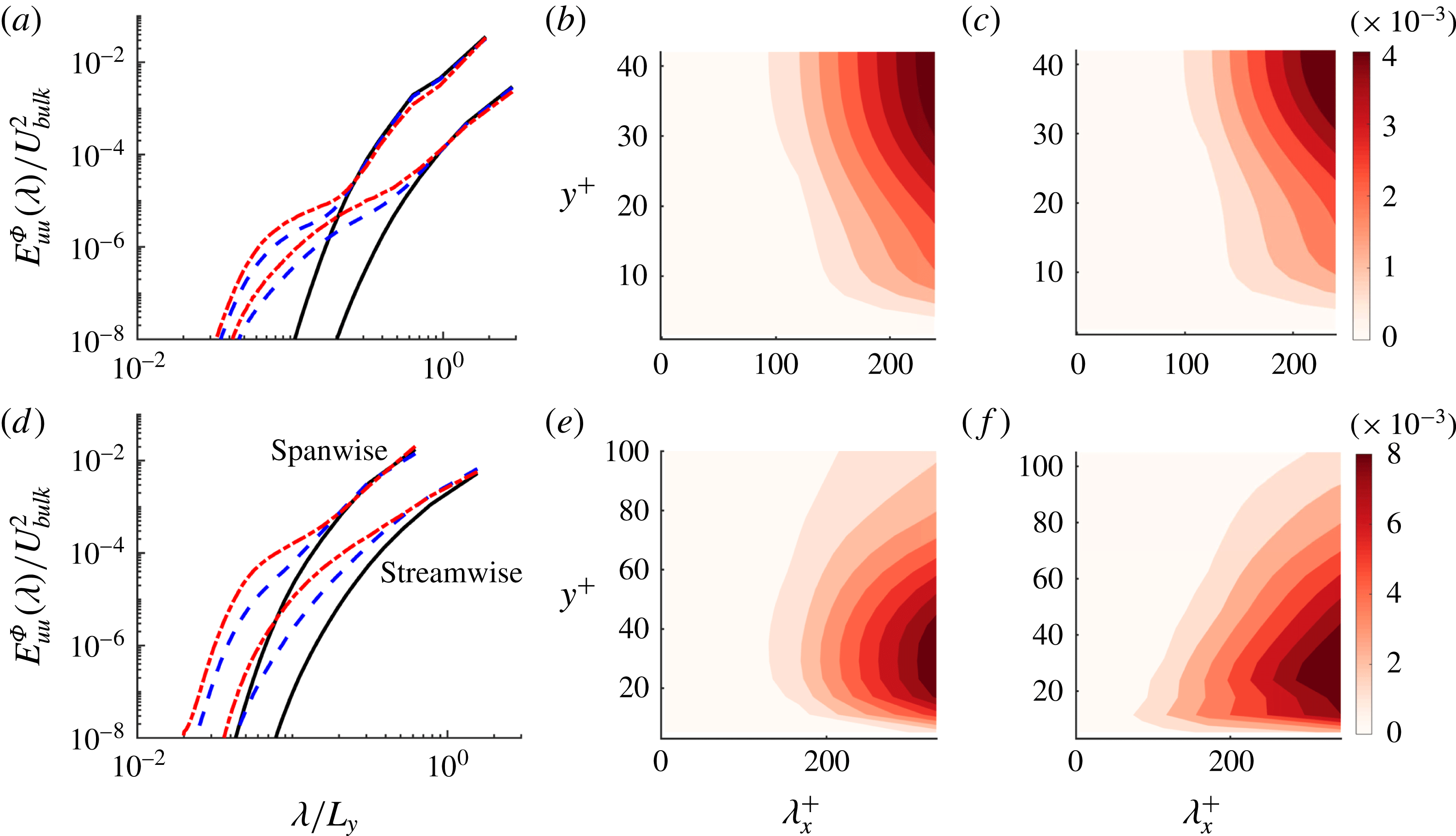
(a–c) Couette flow; (d–f) channel flow. (a,d) The one-dimensional streamwise and spanwise wavenumber energy spectra of the streamwise velocity
 $E_{uu}$
averaged in the wall-normal direction: (a) ——
 $C500-0$
, – – –
 $C500-5$
, – - – -
 $C500-10$
; (d) ——
 $P2600-0$
, – – –
 $P2600-5$
, – - – -
 $P2600-10$
. Contour figures show the two-dimensional contours of the energy spectra. (b,e) Single-phase flow with
 $C500-0$
and
 $P2600-0$
. (c,f) Two-phase flow with
 $C500-5$
and
 $P2600-5$
.

4.3 Energy spectra
The average streamwise energy spectrum
 $E_{uu}^{\unicode[STIX]{x1D6F7}}$
is plotted in figure 9(a,d) as a function of both streamwise and spanwise wavelengths, for both suspension and single-phase flows. One advantage of FCM is that particles are represented in the fluid equations by smooth Gaussian envelope forcing, making this method well suited for spatial Fourier analysis of mixture flow.
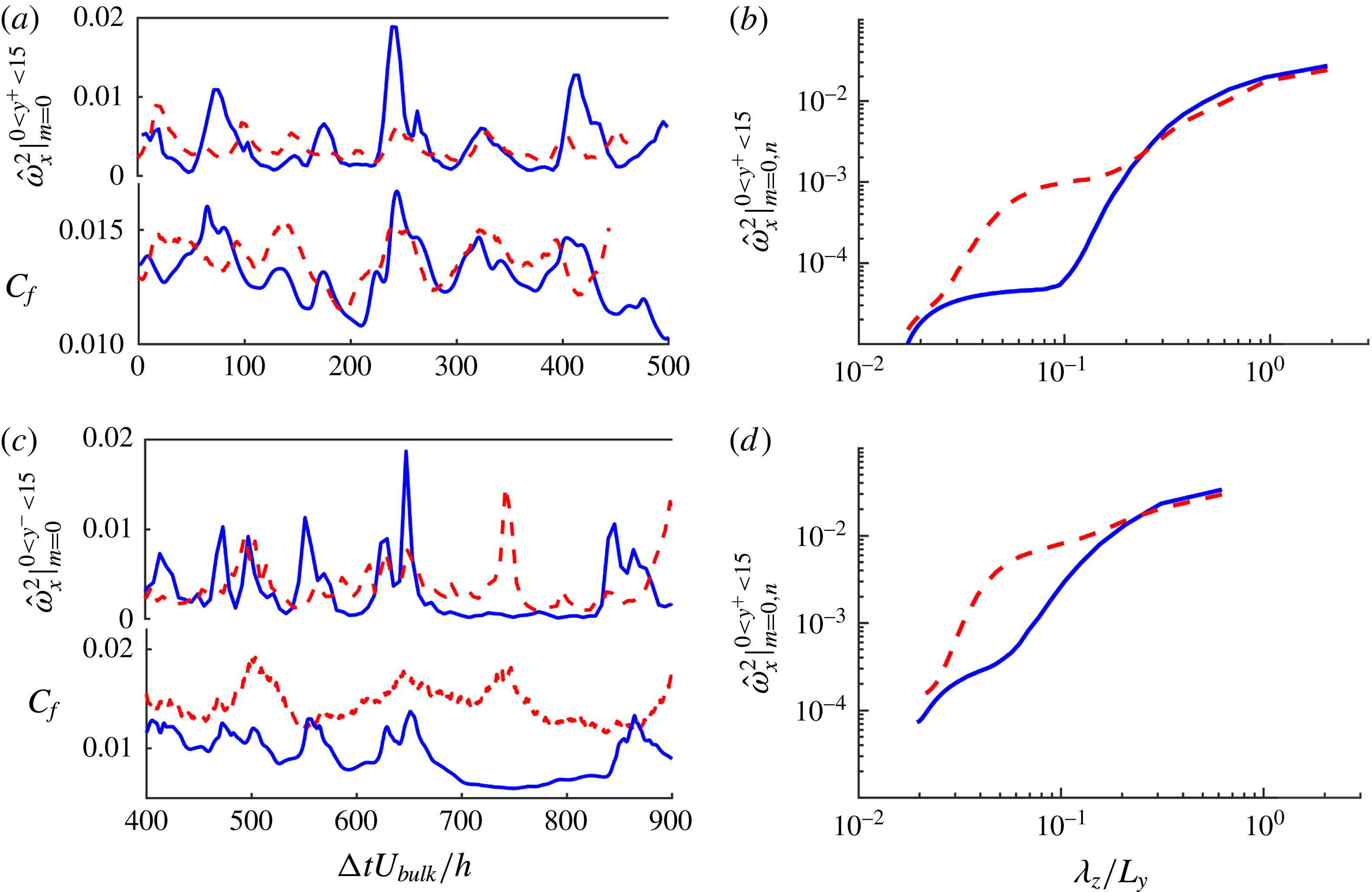
Simultaneous temporal evolution of the friction coefficient
 $C_{f}$
and the near-wall streamwise vorticity, in Couette flow (a,b), and channel flow (c,d). (a,c) Plots of the summation of the amplitude squared of the
 $x$
-independent vortices (
 $m=0$
) for different spanwise wavenumbers (
 $1\leqslant n\leqslant N_{z}/2$
) and integrated in the near-wall region (
 $y^{+}<15$
). (b,d) The
 $x$
-independent vortices (
 $m=0$
) in the near-wall region (
 $y^{+}<15$
) as a function of spanwise wavelength (
 $2L_{z}/N_{z}\leqslant \unicode[STIX]{x1D706}_{z}\leqslant L_{z}$
). The line style indicates single-phase (solid) and two-phase (dashed line) flows: (a,b) ——
 $C500-0$
, – – –
 $C500-5$
; (c,d) ——
 $P2600-0$
, – – –
 $P2600-5$
.

Figure 9(a,d) displays the energy spectra in both flow configurations and for both streamwise and spanwise wavenumbers averaged over the whole domain. Particles strengthen the energy of the flow structures at intermediate scales, especially in the streamwise direction of the channel flow. Moreover, particles hardly affect the energy of the large-scale structures of wavelength
 $3h<\unicode[STIX]{x1D706}_{x}<5.7h$
in Couette flow whereas particles increase the energy contained in
 $h<\unicode[STIX]{x1D706}_{x}<3.1h$
for channel flow. Note that the energy of the fluctuations at small scales in two dimensions (
 $\unicode[STIX]{x1D706}_{x}<d_{p}$
and
 $\unicode[STIX]{x1D706}_{z}<d_{p}$
) might be over-estimated by the numerical method. However, the energy contained in these scales obtained from two-dimensional modal analysis is
 $10^{-7}\,\%$
(respectively
 $10^{-4}\,\%$
) of the energy of the largest scales in Couette (respectively channel) flow, and therefore the errors introduced by small scales on the analysis of energy spectra can be neglected.
The energy spectra in the streamwise direction are plotted as a function of the wall-normal position in figure 9(b,c,e,f). It is interesting to note in figure 9(b,c) that the most energetic large-scale motion in Couette flow is found in the range
 $20<y^{+}<40$
, which corresponds to the buffer layer region. The extent of the most energetic eddies is slightly shrunk towards the Couette flow centre by the presence of the particle.
In channel flow the most energetic flow structures (
 $h<\unicode[STIX]{x1D706}_{x}<3h$
) are located at
 $10<y^{+}<50$
as shown in figure 9(e,f). Contrary to Couette flow, finite-size particles in channel flow enhance the strength of moderate streamwise vortices in comparison to single-phase flow. The energy of these streamwise vortical structures subsequently increases the flow velocity gradient near the wall, as will be shown in figure 10. The energy modulation near the walls (
 $y^{+}<20$
) is due to the interaction of the particles with the streaks rather than their interaction with the large-scale vortices. Two indirect pieces of evidence may support this conclusion. First, particles in Couette flow do not generate significant modulation near the walls (
 $y^{+}<20$
) in figure 9(c) when particles are in large-scale vortices. Second, in channel flow, we also observe the generation of vortical energetic structures when particles are seeded in the bottom wall only with artificial streaks (as shown in figure 4
c).
5 Modification of the regeneration cycle by particles
The period of the regeneration cycle can be identified from the low frequency evolution of the friction coefficient signal or Reynolds shear stress. First, the effect of the particles on the intermittency of the flow will be characterized by considering the fluctuation in time of the friction coefficient and Reynolds shear stress. Second, their impact on the successive sub-processes of the regeneration cycle will be qualitatively detailed in the following subsections, considering (I) the lift-up mechanism yielding streak formation, (II) the modal analysis of flow velocity fluctuations for its indication on the correlation between the
 $x$
-dependent (
 $m>0$
and
 $n\geqslant 0$
) and
 $x$
-independent (
 $m=0$
and
 $n>0$
) streaks, and (III) the vorticity stretching and vortex regeneration.
5.1 Wall friction coefficient and streamwise vorticity
The friction coefficient is a dimensionless measure of the wall shear stress. The temporal evolution of the friction coefficient is displayed in figure 10. For Couette flow, the average friction coefficient and temporal fluctuations are slightly increased by the presence of particles, whereas for channel flow the increase of the average friction coefficient is more significant, and the fluctuation amplitude is slightly reduced. The increase of friction coefficient cannot be exclusively related to the increase of the suspension effective viscosity. Indeed the ratio of the time-averaged friction coefficient of the suspension to single-phase flow is around
 $1.4$
, whereas the viscosity increase due to the particle presence is around
 $1.14$
. Recent work from Costa et al. (Reference Costa, Picano, Brandt and Breugem2016) provided a theoretical prediction of the total suspension drag. Predicted
 $Re_{\unicode[STIX]{x1D70F}}$
is
 $103$
based on suspension viscosity, where
 $Re_{\unicode[STIX]{x1D70F}}$
is
 $109$
based on DNS in table 1.
Jiménez & Moin (Reference Jiménez and Moin1991) have explicitly shown that the maximum (in time) of the wall shear stress is synchronous with the maximum near-wall vorticity (
 $0<y^{+}<10$
). Using two-dimensional numerical simulations (neglecting the variation in the streamwise direction), Orlandi & Jiménez (Reference Orlandi and Jiménez1994) showed that the transport of fluid from longitudinal vortices to the high- and low-speed streaks is the origin of the higher wall friction in turbulent layers, especially in the sweep region where high-speed fluid is transported towards the wall. Therefore large-scale streamwise vortical structures control the near-wall velocity gradient. Figure 10(a,c) shows simultaneously the evolution of the wall friction coefficient and the summation over all of the spanwise wavenumbers for
 $x$
-independent vorticity
 $\hat{|\unicode[STIX]{x1D714}|}_{x,wall}^{2}\equiv \sum _{n=1}^{N_{z}/2}\int _{0}^{y^{+}=15}\hat{|\unicode[STIX]{x1D714}|}_{x}^{2}(0,n\unicode[STIX]{x1D6FD})\,\text{d}y$
, where the mode
 $(0,n\unicode[STIX]{x1D6FD})$
with
 $n\neq 0$
corresponds to an
 $x$
-independent structure. The cross-correlation between
 $C_{f}$
and
 $\hat{|\unicode[STIX]{x1D714}|}_{x,wall}^{2}$
is calculated following (5.1), where the prime denotes the temporal fluctuation of a quantity and the overline indicates the average over time:
 $$\begin{eqnarray}R=\frac{\overline{(C_{f})^{\prime }\cdot (\hat{|\unicode[STIX]{x1D714}|}_{x,wall}^{2})^{\prime }}}{(C_{f})_{rms}\cdot (\hat{|\unicode[STIX]{x1D714}|}_{x,wall}^{2})_{rms}}.\end{eqnarray}$$
The cross-correlation gives
 $R=0.51,0.49,0.63,0.68$
for the respective flow configurations
 $C500-0,C500-5,P2600-0,P2600-5$
. Clearly, there is a correlation in time between the instantaneous wall friction coefficient and the near-wall streamwise vorticity in all cases. The spectra of near-wall streamwise vorticity
 $\hat{|\unicode[STIX]{x1D714}|}_{x,wall}^{2}$
are shown in figure 10(b,d) for both single-phase and suspension flows. The ratio of the vorticity at small scales (
 $\unicode[STIX]{x1D706}_{z}/L_{y}<0.2$
) to the largest-scale streamwise vortices is much smaller in Couette flow than in channel flow (the ratios are
 $O(0.01)$
and
 $O(0.1)$
respectively). In two-phase flows, turbulence becomes more isotropic, because particles inject energy in small scales, which is transferred back to intermediate scales. This is for example the case in the work of Elghobashi & Truesdell (Reference Elghobashi and Truesdell1993), even though the origin of momentum transfer is not the same; there is slip between the phases in their work, whereas in our work the interactions are mainly due to the finite size of the particles. The streamwise vorticity is enhanced at low spanwise wavelengths (
 $\unicode[STIX]{x1D706}_{z}/L_{y}<0.2$
, which corresponds to
 $\unicode[STIX]{x1D706}_{z}/d_{p}<4$
) in both configurations. The enhancement is of one order of magnitude in Couette flow, and of two orders of magnitude in channel flow.
5.2 Reynolds shear stress
From the investigation of total energy input and dissipation rate, Kawahara & Kida (Reference Kawahara and Kida2001) evidenced the temporal evolution of spatial structures in a cyclic sequence consistent with the regeneration cycle proposed by Hamilton et al. (Reference Hamilton, Kim and Waleffe1995). A strong ejection event is followed by a gradual decrease of intensity over a certain period of time. The maximum (in time) of the Reynolds stress occurs when the dissipation rate is large along the periodic orbit. The quasi-periodicity of the turbulent events can be represented by the spatio-temporal evolution of the Reynolds stress
 $-\overline{u^{\prime }v^{\prime }}(y,t)$
across the Couette gap or channel height, as shown in figure 11. Note that the period of turbulent events is of
 $O(100)$
time units in both flows. This characterizes the time needed for the velocity fluctuations to become uncorrelated in time. The particle Stokes number which can be based on this time scale is very small compared to the one related to the shear.
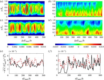
Spatio-temporal evolution of the Reynolds shear stress (
 $-\overline{u^{\prime }v^{\prime }}/U_{bulk}^{2}$
) averaged in the homogeneous directions (streamwise and spanwise) in (a–d); its average within
 $5<y^{+}<30$
is shown in (e,f). (a,c,e) Couette flow and (b,d,f) channel flow. Panels (a,b) correspond to single-phase flows whereas (c,d) correspond to two-phase flows; (e) ——
 $C500-0$
and – – –
 $C500-5$
; (f) ——
 $P2600-0$
and – – –
 $P2600-5$
.

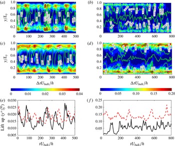
For Couette flow, the maximum of the Reynolds stress is located in the centre of the gap. The two walls share one buffer layer and a couple of central large-scale vortices, with a strong coupling between the streaks near the walls. The low-speed streak near one wall ejects fluid to the other wall, acting there as a high-speed streak. It is revealed by figure 11(a,c,e) that neutrally buoyant particles have a negligible effect on both the intensity and intermittency of the Reynolds stress in the Couette flow configuration (Wang et al. Reference Wang, Abbas and Climent2017). The channel flow contains a log-law region and the central region is ruled by the velocity defect law. Figure 11(b) shows that the strongest shear stress bursts are located close to the channel walls, and that the frequency of these bursts is of the same order of magnitude as in Couette flow. In the presence of neutrally buoyant particles, the intensity of the Reynolds shear stress is enhanced, as shown in figure 11(d), and the frequency of these events is decreased, as shown in figure 11(f). The increase of Reynolds shear stress is closely correlated with the sweep events, as indicated in figure 7(d), making the friction coefficient and Reynolds shear stress fluctuations synchronous.
5.3 Streak formation: the lift-up mechanism
The streaks form on both sides of a vortex. Low-speed fluid is lifted up away from the wall by the vortex into a region of higher-speed fluid, producing a low-speed streak, while on the other side of the vortex, high-speed fluid is pushed towards the wall, creating a high-speed streak. Ellingsen & Palm (Reference Ellingsen and Palm1975) have shown, using a linear stability analysis, that the
 $x$
-independent streamwise perturbations grow linearly in time as
 $-v(\text{d}\overline{u}/\text{d}y)t$
(the so-called lift-up effect), making any shear flow
 $\overline{u}(y)$
unstable to
 $x$
-independent (transverse) perturbations. Consequently, in shear flows, the main linear mechanism for transient disturbance growth is the lift-up effect which produces high- and low-speed streaks in the streamwise velocity. Bech et al. (Reference Bech, Tillmark, Alfredsson and Andersson1995) stated that the inner shear layer is formed through the lift-up of low-speed streaks from the viscous sublayer; then the shear layers are coupled to an instantaneous velocity profile with inflectional character and they have been observed to become unstable and break up into chaotic motion, so-called ‘bursting’. The lift-up effect or advection was identified as a robust mechanism for the generation of the streaky motions in both transitional and turbulent flows (Ellingsen & Palm Reference Ellingsen and Palm1975; Hamilton et al.
Reference Hamilton, Kim and Waleffe1995; Del Álamo & Jiménez Reference Del Álamo and Jiménez2006).
Spatio-temporal evolution of the lift-up term (
 $-v\text{d}\overline{u}/\text{d}y$
) scaled by
 $U_{bulk}^{2}/h$
. The green isoline of the Reynolds shear stress (
 $-\overline{u^{\prime }v^{\prime }}/U_{bulk}^{2}$
) is added on the top of these figures; the interval in (a,c) is
 $0.003$
, and the interval in (b,d) is
 $0.005$
. (a,c,e) Couette flow and (b,d,f) channel flow. (a,b) Single-phase flows; (c,d) two-phase flows. The average of the lift-up term within
 $5<y^{+}<30$
is shown in (e,f): (e) ——
 $C500-0$
and – – –
 $C500-5$
; (f) ——
 $P2600-0$
and – – –
 $P2600-5$
.

Klinkenberg et al. (Reference Klinkenberg, Sardina, De Lange and Brandt2013) have shown that small pointwise inertial particles do affect the transition to turbulence, not by altering the lift-up effect but rather by modifying the dynamics of the oblique waves necessary for the streak regeneration and breakdown. In order to show whether finite-size particles modify the lift-up term, the contours of
 $-v\,\text{d}\overline{u}/\text{d}y$
are displayed in figure 12 together with the isolines of the Reynolds shear stress (from figure 11). The lift-up term is important near the walls in both flow configurations. For Couette flow, the contours shown in figure 11(a,c) are not significantly modified by the presence of the particles. Based on figure 11(a,c), which plots the averaged value within
 $5<y^{+}<30$
, we can observe that the strongest effects are nearly the same with or without particles, whereas the weakest effects are enhanced by the particles. However, in channel flow within the buffer layer (
 $5<y^{+}<30$
), the particles not only enhance the lift-up significantly, but also let it act continuously (the lift-up effect is less frequent in suspension flow, as shown in figure 11
f).
5.4 Streak breakdown: modal decomposition of the fluctuating energy
The subsequent process is the instability of
 $x$
-independent streaks, the so-called streak breakdown. Hamilton et al. (Reference Hamilton, Kim and Waleffe1995) have shown that it is the instability of the streaks (through a nonlinear process) which causes breakdown. We investigated the temporal evolution of the energy contained in the dominant flow fluctuation modes, since it can give evidence on the dynamics of the streak breakdown process, and on the particle modulation of this process.
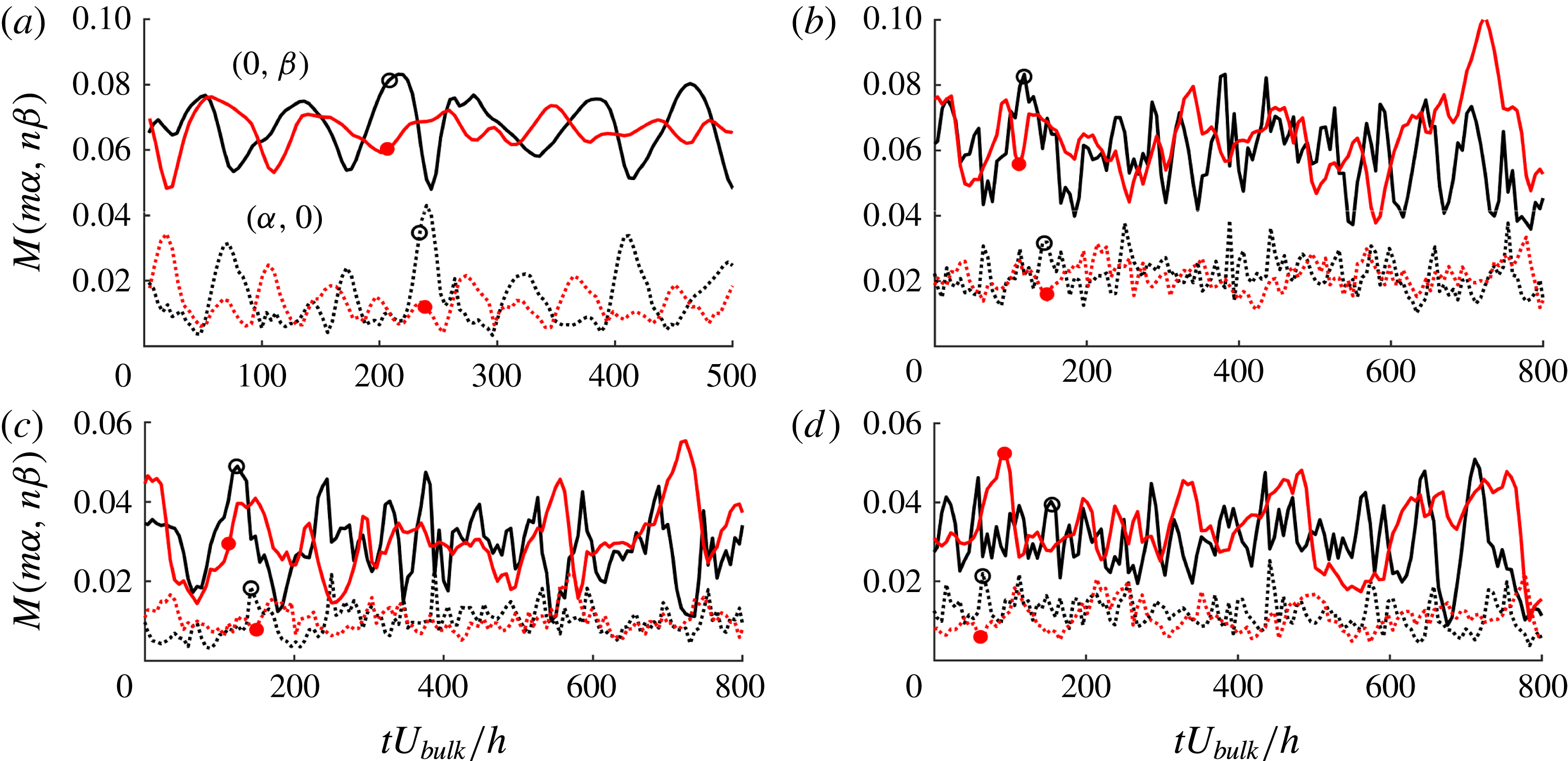
Modal decomposition as in (4.1): —— mode
 $M(0,\unicode[STIX]{x1D6FD})$
;
 $\cdots \cdots$
mode
 $M(\unicode[STIX]{x1D6FC},0)$
. (a) Couette flow in the whole domain, (b) channel flow in the whole domain, (c,d) channel flow in the upper half-domain and bottom half-domain. (a) Black is
 $C500-0$
and red is
 $C500-5$
. (b–d) Black circles are
 $P2600-0$
and red discs are
 $P2600-5$
.

The temporal evolution of the most energetic modes is shown in figure 13. In figure 13(a,b), (4.1) is integrated between the two walls (
 $Y_{1}=0$
and
 $Y_{2}=L_{y}$
), whereas in figure 13(c,d), the integration is performed in the vicinity of one single wall, which is regarded as an individual shear layer (
 $Y_{1}=0\rightarrow Y_{2}=L_{y}/2$
near the bottom wall, and
 $Y_{1}=L_{y}/2\rightarrow Y_{2}=L_{y}$
near the upper wall). The quasi-periodic fluctuations of these modes, with period
 ${\sim}100h/U_{bulk}$
for Couette flow, are related to the regeneration cycle. The strongest mode is
 $M(0,\unicode[STIX]{x1D6FD})$
which corresponds to
 $x$
-independent streaks. As a general trend, neutrally buoyant particles decrease the amplitude of the fluctuations of this mode, whereas they do not have significant impact on its period, which is related to the regeneration cycle. However, in channel flow, it can be noted that both the
 $(0,\unicode[STIX]{x1D6FD})$
mode and
 $(\unicode[STIX]{x1D6FC},0)$
mode are of the same strength and period compared between single- and two-phase flow.
In Couette flow, one can note the relation of the intermittency of modes
 $(0,\unicode[STIX]{x1D6FD})$
(
 $x$
-independent) and
 $(\unicode[STIX]{x1D6FC},0)$
(
 $x$
-dependent), when integrated over the entire gap. The correlation between the different modes calculated similarly to (5.1) gives
 $R=-0.64$
for single-phase Couette flow (
 $C500-0$
) and
 $-0.59$
for suspension flow (
 $C500-5$
). The values of
 $R$
are negative, showing the clear anti-correlation between the two modes. The peaks of
 $M(0,\unicode[STIX]{x1D6FD})$
correspond to instants at which the streaks have the least
 $x$
-dependence. As the streaks become wavy,
 $M(0,\unicode[STIX]{x1D6FD})$
decreases, while the energy of
 $M(\unicode[STIX]{x1D6FC},0)$
(the fundamental mode in the
 $x$
-direction with no spanwise variation) sharply increases. The other
 $(\unicode[STIX]{x1D6FC},n\unicode[STIX]{x1D6FD}),n\neq 0$
modes can hardly be distinguished. Breakdown occurs when
 $M(0,\unicode[STIX]{x1D6FD})$
reaches a minimum. The amplitude of both mode fluctuations is slightly damped by the particle presence, as shown in figure 13(a).
For channel flow, figure 13(b) shows higher frequency fluctuations than in Couette flow, and less correlation between the
 $(\unicode[STIX]{x1D6FC},0)$
and
 $(0,\unicode[STIX]{x1D6FD})$
modes, when integrated over the whole domain. This is due to two coexisting shear layers (one at each wall) which are relatively independent of each other (turbulent mixing is weak in the core region between the two shear layers at low Reynolds number). When the modal energy is integrated over half of the channel section, as shown in figure 13(c,d), one can notice a stronger correlation between the
 $(0,\unicode[STIX]{x1D6FD})$
mode and
 $(\unicode[STIX]{x1D6FC},0)$
mode, as in Couette flow, although this is less pronounced in channel flow. The particles do not have a strong effect on the temporal evolution of these modes, suggesting that particles do not significantly alter the breakdown process.
5.5 Vortex regeneration: nonlinear interaction and vortex stretching
During streak breakdown, a complex set of interactions reinforces the streamwise vortices, leading to the formation of a new set of streaks, and completing the regeneration cycle. Hamilton et al. (Reference Hamilton, Kim and Waleffe1995) proposed that the vortex strengthening is due to interactions among the
 $\unicode[STIX]{x1D6FC}$
-modes, which grow during the streak breakdown. Schoppa & Hussain (Reference Schoppa and Hussain2002) suggested that the vortex formation is inherently three-dimensional, with a direct stretching (inherent to streak
 $(x,z)$
-waviness) of the near-wall
 $\unicode[STIX]{x1D714}_{x}$
sheets, leading to the collapse of streamwise vortices. They provided insights into the dynamics of near-wall vortex formation through the inviscid balance of the streamwise vorticity:
 $$\begin{eqnarray}\frac{\unicode[STIX]{x2202}\unicode[STIX]{x1D714}_{x}}{\unicode[STIX]{x2202}t}=\underbrace{-u\frac{\unicode[STIX]{x2202}\unicode[STIX]{x1D714}_{x}}{\unicode[STIX]{x2202}x}-v\frac{\unicode[STIX]{x2202}\unicode[STIX]{x1D714}_{x}}{\unicode[STIX]{x2202}y}-w\frac{\unicode[STIX]{x2202}\unicode[STIX]{x1D714}_{x}}{\unicode[STIX]{x2202}z}}_{advection}+\underbrace{\unicode[STIX]{x1D714}_{x}\frac{\unicode[STIX]{x2202}u}{\unicode[STIX]{x2202}x}}_{stretching}+\underbrace{\frac{\unicode[STIX]{x2202}v}{\unicode[STIX]{x2202}x}\frac{\unicode[STIX]{x2202}u}{\unicode[STIX]{x2202}z}-\frac{\unicode[STIX]{x2202}w}{\unicode[STIX]{x2202}x}\frac{\unicode[STIX]{x2202}u}{\unicode[STIX]{x2202}y}}_{tilting}.\end{eqnarray}$$
In fully developed turbulence, the greatest contribution, in magnitude, to the temporal evolution of the vorticity
 $\unicode[STIX]{x2202}\unicode[STIX]{x1D714}_{x}/\unicode[STIX]{x2202}t$
comes from the tilting term. This is confirmed by our simulations (not shown here). However Schoppa & Hussain (Reference Schoppa and Hussain2002) have stated that this term contributes to the thin tail of the near-wall
 $\unicode[STIX]{x1D714}_{x}$
layer, and is not responsible for the formation of
 $x$
-independent streamwise vortices (
 $(0,\unicode[STIX]{x1D6FD})$
mode in miniunit). Instead, the vortex formation is dominated by the stretching of the streamwise vorticity. The local
 $\unicode[STIX]{x1D714}_{x}$
stretching is sustained in time and is mainly responsible for the vortex collapse, whose location coincides with the
 $+\unicode[STIX]{x1D714}_{x}\unicode[STIX]{x2202}u/\unicode[STIX]{x2202}x$
peak. The streak meandering provides the generation of
 $\unicode[STIX]{x2202}u/\unicode[STIX]{x2202}x$
. Then direct stretching of positive and negative
 $\unicode[STIX]{x1D714}_{x}$
occurs in regions where
 $\unicode[STIX]{x2202}u/\unicode[STIX]{x2202}x$
is generated across the wavy streak flanks during the streak breakdown process. The stretching term is active only during the peaks of the cycle when local three-dimensionality is induced after streak breakdown (see Jiménez & Moin Reference Jiménez and Moin1991).
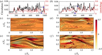
Evidence of the particle influence on the vorticity stretching in channel flow. (a,c,e,) Single-phase flow
 $P2600-0$
; (b,d,f) suspension flow
 $P2600-1$
. (a,b) The evolution in time of both —— the circulation and
 $\cdots \cdots$
the vorticity stretching
 $|\unicode[STIX]{x1D714}_{x}\unicode[STIX]{x2202}u/\unicode[STIX]{x2202}x|$
. Both are averaged within the region
 $0.1<y/L_{y}<0.4$
where large-scale vortices take place, as seen in figure 5(b). (c–f) The streamwise velocity fluctuations in the plane
 $y/L_{y}=0.2$
, using
 $\cdots \cdots$
for negative isolines and – – – for positive isolines, with a step equal to 0.04. The contours indicate the stretching term
 $\unicode[STIX]{x1D714}_{x}\unicode[STIX]{x2202}u/\unicode[STIX]{x2202}x$
. The instants corresponding to the different snapshots are marked in (a,b). Panels (c,d) correspond to a trough of the vorticity stretching whereas (e,f) correspond to a peak of the vorticity stretching.

In our previous paper (Wang et al.
Reference Wang, Abbas and Climent2017), we have shown that the streak waviness and vorticity stretching are almost unchanged for Couette flow in the presence of neutrally buoyant particles. However, in channel flow, the particles have some impact. Figure 14(a,b) shows the temporal evolution of the circulation as well as the vorticity stretching term, for both single- and two-phase channel flows. The vorticity stretching (averaged value is
 $0.17$
(respectively
 $0.11$
) for
 $P2600-1$
(respectively
 $P2600-0$
)) and the circulation (averaged value is
 $0.025$
(respectively
 $0.02$
) for
 $P2600-1$
(respectively
 $P2600-0$
)) are enhanced near the channel walls due to the presence of the particles. The cross-correlation between them was calculated, as in (5.1), giving
 $0.576$
for
 $P2600-0$
and
 $0.624$
for
 $P2600-5$
. This shows that high flow circulation is synchronized with the appearance of
 $x$
-dependent flow structures. Figure 14(c–f) shows instantaneous snapshots containing the contours of the streamwise velocity fluctuations (that illustrate the streak shape), as well as the vorticity stretching. These snapshots are taken at high vorticity stretching (high flow circulation). They show clear evidence that nonlinear processes such as streak breakdown, and thereby vortex regeneration, take place in the suspension flow as in single-phase flow. They also show that the wavy streaks are smaller and more numerous in suspension flow, when compared to the single-phase flow.
6 Concluding remarks
We have studied turbulent suspension flows in plane Couette and pressure-driven (channel) configurations, slightly above the laminar–turbulent transition. The fundamental difference between the two flow configurations, for weak turbulence, is due to the shear layers. In turbulent plane Couette flow there is only one shear layer and a single regeneration cycle, whereas there are two shear layers and two relatively independent regeneration cycles in turbulent channel flow (one on each wall). Dilute to moderately concentrated suspensions of neutrally buoyant finite-size spherical particles were considered, the particle diameter being twenty times smaller than the Couette gap or channel height. The simulation domain was chosen to ensure a minimal set of coherent flow structures sufficient to sustain turbulence in both flow configurations.
The effect of particles on the transition was first examined. Different initial combinations
 $\{\text{flow}+\text{particles}\}$
were considered to support our intention to show that the difference in the flow response in Couette and channel configurations, when particles are added, is essentially correlated to the particle spatial distribution. In Couette flow, the streak generation from large-scale rolls is a very robust mechanism in single-phase flow. For example, when the streaks were removed from fully developed turbulence, the streaks in single-phase flow were immediately regenerated (see Hamilton et al.
Reference Hamilton, Kim and Waleffe1995). When particles were added to the flow from which the streaks have been removed (weak turbulence in Couette flow), the flow could hardly recover the turbulence features in time if the particles were seeded in the large-scale rolls. However, the streaks were regenerated if the particles were seeded initially within the streaks and forced (artificially) to stay there. On the contrary, in channel flow, the artificial streak we used is known to damp over time if the flow is particle-free (Schoppa & Hussain Reference Schoppa and Hussain2002). Whenever particles were added into that structure (even at low overall concentration), the energy of this artificial streak grew, leading to transition. If the particles were randomly seeded (with the same average concentration), the flow became laminar.
In the turbulent regime, detailed temporal and spatial analysis, in physical and Fourier space, were proposed. The statistics of the flows laden with particles were formed at effective Reynolds numbers 40 %–50 % larger than the critical effective Reynolds number for each flow (‘effective’ means that the additional dissipation due to the presence of the particles is taken into account in the suspension flow viscosity). Particles did not modify significantly the features of plane Couette flow, whereas they had a clear impact on channel flow. The particle spatial distribution was found to be non-uniform over the cross-section. Particles were more present in the core of the large-scale rolls (inactive motion) in Couette flow, and in the ejection (active motion) regions in channel flow. This finding is essentially related to the wall-normal inertial lift forces (on finite-size particles) that act in opposite directions depending on the flow configuration.
Contrary to Couette flow, the accumulation of particles in the active region of turbulence regeneration for the channel flow configuration yielded clear modifications of the flow statistics and a dynamical response. We observed a reduction of streamwise velocity r.m.s. and an increase of the wall-normal component. The wall shear stress was also significantly increased because particles had reinforced the activity of larger-scale
 $x$
-independent streamwise vortices near the walls.
The regeneration cycle of wall turbulence has been studied in the presence of particles. Despite the universality of wall turbulence, the Couette flow is constituted of a single shear layer whereas channel flow has two shear layers with opposite signs, leading to a different flow response to perturbations. The three successive sub-steps of the regeneration cycle were modified by finite-size particles, since they actively contribute to the dynamics of the buffer layer. We observed an enhancement of the lift-up mechanism together with a reinforced Reynolds shear stress (although the frequency of burst events was decreased). Vorticity stretching was increased, leading to smaller and more numerous wavy streaks for pressure-driven two-phase flow. Thanks to their preferential presence near the walls, particles triggered small-scale vortices that were stretched by the shear flow and survived even at Reynolds numbers below the transition limit of single-phase flow. By studying two distinct turbulent flow configurations laden with neutrally buoyant finite-size particles, we were able to show the specific response of turbulent structures and the modulation of the fundamental mechanisms composing the regeneration cycle of near-wall turbulence.
Acknowledgements
This work was granted access to the HPC resources of CALMIP under the allocation 2015 and 2016-P1002 and of GENCI under the allocation x20162b6942. We are grateful to COST Action MP1305 on Flowing Matter. Great help from A. Pedrono for technical support on JADIM is also acknowledged.