

1. Introduction
Careful analysis of the adjustment impacts of trade reform is essential to policy makers in developing countries as they seek to improve the structure of incentives within an outward looking trade and competitiveness strategy. An immediate concern, especially in low-income countries, is the impact of tariff liberalization on tax revenues. Tariffs are typically an important source of tax revenues in low-income countries, often reflecting the weakness of the domestic tax base and of other tax instruments. In addition, changes in output in different sectors and associated impacts on employment are likely to be an important aspect of the political economy driving support and opposition to trade reform. Further, trade reform entails changes in prices and an important consideration is how these will affect households, especially the poorest. A good understanding of the potential adjustment implications of trade reform can contribute to the design of better trade reform strategies and to the discussion and implementation of policies that can reduce the impact of adjustment, especially when the costs are concentrated upon particular groups in society. The latter is of particular importance in countries that lack social safety nets with broad coverage.
In response, the World Bank has developed a simple spreadsheet tool called TRIST (Tariff Reform Impact Simulation Tool) that can be used in client countries to analyze the short-term adjustment implications of tariff reform.Footnote 1 The tool was developed to provide better estimates to policy makers and trade negotiators in developing countries of the impact of changes in tariffs on government revenues, imports, protection, and prices in the short run, taking advantage of the more detailed information on imports that is increasingly available at the country level from computerized customs systems. TRIST does not require any proprietary software, programming skills or internet access. It is free and easy to use, transparent, with a simple underlying trade model, and flexible in that it can quickly address different trade policy scenarios. It uses detailed data on actual revenues collected on imports, whereas other tools use hypothetical revenues from applying duty rates on paper. It can take into account all official taxes levied on imports at the border, not just tariffs, and show the change in trade tax revenues, which is more relevant than the change in tariff revenues alone. When suitable data are available, it can provide information on the short-term relative vulnerability of different sectors in the domestic economy in terms of output and employment. It can also be linked to household budget data to trace the influence of changes in prices following trade reform to household expenditures and the costs of attaining a given consumption bundle.
TRIST is a partial equilibrium model and there are naturally issues that the model is not well suited to answer. It cannot be used to project the aggregate impact of tariff reform. Thus, it cannot provide an assessment of whether a particular policy change is beneficial or not. This would require a more sophisticated economy-wide model.
This paper provides a description of the TRIST tool and gives examples of its use. Section 2 discusses the objective behind the development of TRIST and outlines crucial advantages compared to existing tools. Section 3 presents the trade model underlying the tool and discusses the intuition behind the calculation steps. In Section 4, some examples of the analysis of short-term adjustment costs using TRIST are presented. Section 5 concludes.
2. The purpose of TRIST
The TRIST software is open-source and free of charge. The tool is Excel based and does not require any additional proprietary software, hardware (other than minimal disk space), or programming expertise. The origin of TRIST lies in the limitations of existing tools in providing support to policy makers in developing countries in assessing the implications of tariff reforms and the opportunities created by the increasing use of computerized customs systems to deliver data that are more relevant for detailed analysis of revenue impacts. There are three main features of TRIST:
1. Most tools for trade policy analysis use statutory tariff rates (those on paper) and recorded trade flows. This can lead to a lack of precision in predicted impacts since a common feature of import regimes of developing countries is the widespread use of tariff exemptions. For example, a range of institutions including the government, international agencies, embassies, and NGOs (non-governmental organizations) usually do not pay duties on products imported for official purposes. It is important that these imports are excluded since they do not generate revenue for the government, do not enter the domestic market in free circulation, and cannot be used for commercial purposes. Exemptions are also granted on imported intermediate products and capital goods to provide incentives for exports and for domestic and foreign investment. Hence, it is important to take these exemptions into account and assess their importance.Footnote 2 TRIST is designed to use both statutory and applied tariff data and is able to assess the impact of tariff exemptions. In this regard, for the low-income countries for which TRISTs have been developed, we find that exemptions can amount to 40–50% of total revenue collected. These numbers illustrate that a better understanding of the magnitude and structure of tariff exemptions is crucial in determining the adjustment implications of tariff reform on fiscal revenues.
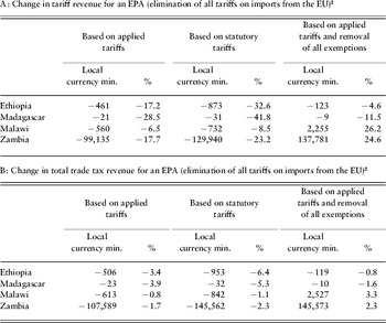
Using statutory rather than actually applied duties to investigate the impact of tariff liberalization scenarios will typically lead to a substantial overestimation of the impact of tariff liberalization on trade flows and revenues. Table 1 shows how tariff and total trade tax revenue in selected Common Market for Eastern and Southern Africa (COMESA) countries would be affected by the removal of tariffs on imports from the EU under an economic partnership agreement (EPA). We assume here that the EPA entails reducing all tariffs on products imported from the EU to zero. In practice, there are likely to be a range of products that are excluded that will reduce the revenue effect, so that the estimates here will provide an upper bound on actual impacts.Footnote 3 Column one in part A of the table shows that the predicted changes in tariff revenues when using applied tariff rates amount to around 17%–18% for Ethiopia and Zambia, 30% for Madagascar, and 6% for Malawi. The next column in part A presents the tariff revenue loss predicted when statutory tariff rates are used as in previous studies. It is clear that the predicted losses are now substantially higher. The final column in part A of Table 1 examines a scenario in which the respective countries attempt to recover the revenue loss they incur due to the EPA by abolishing all tariff exemptions on products that enter the domestic market. The numbers show that the resulting tariff revenue loss is much lower and there is even a gain in revenues in Zambia and Malawi.
Highlighting the features of TRISTFootnote 1

Notes: 1 The demand elasticity is set to 0.5, the exporter substitution elasticity is set to 1.5.
2 EPA scenario: zero tariffs with EU. For all other trading partners, tariffs are unchanged.
2. A second major challenge in investigating the impact of trade policy reform is to account not only for statutory and applied tariff rates, but also for the interplay between tariffs and other forms of taxes levied on imports. Whilst customs duties are a key source of revenue in developing countries, they represent just one of potentially many taxes and charges levied on imports. Most countries also apply excise taxes as well as a VAT or sales tax.Footnote 4 Often these will generate significantly more revenue than customs duties. In fact, our estimates show that in most countries tariff revenue constitutes substantially less than 50% of overall revenue collected at the border, for example Bolivia (20%), Kenya (25%), Mozambique (32%), and Burundi (39%). In practice, the domestic tax base – for VAT in particular – tends to be very small in developing countries. Thus, it is very important to take into account changes in VAT and excise receipts that follow the reform of customs duties, since it is total revenues from trade that are of interest to policy makers.
Part B of Table 1 presents the impact of the EPA policy scenario on overall import tax revenues. The predicted percentage change in overall tax revenues at the border is substantially less than the percentage change in tariff revenues that is typically presented in studies of the revenue impact of trade reform. The total revenue losses increase slightly in the case of all four countries considered in Table 1. However, it is not clear ex-ante whether the effect of trade liberalization on VAT and excise revenue will be positive, due to increased imports, or negative, due to a reduction of the tax base, since VAT is usually levied on the tariff inclusive value of imports. Changes can also result from trade diversion if the collection rate for these taxes varies significantly between imports from different trading partners. Either way, studies that focus solely on changes in customs duties will provide only a partial and potentially misleading picture.
3. A third major motivation for the development of TRIST is the limitations that arise from using aggregated and unwieldy models in a dynamic policy environment. New options and proposals for trade policy emerge frequently and require adjustments to the scenarios used for projections. Further, trade policy discussions typically concern detailed products, such as identifying lists of sensitive products that are excluded from liberalization scenarios. Thus, disaggregated results that break down the revenue impact by detailed product and trading partner are a crucial input to trade policy formulation. An important aim of TRIST is to provide a simple and flexible tool that can be easily and quickly used and adapted to reflect specific country circumstances as well as to allow the user to define relevant reform scenarios, exclusion lists, etc. Of course, such a tool has its limitations. Using a simple partial equilibrium model like TRIST involves trade-offs compared to using more aggregated less flexible economy-wide general equilibrium (GE) models. TRIST addresses questions related to detailed trade policy changes, but it does not capture inter-sectoral effects or long-term aggregate impacts.
One example of the need for such flexibility is the definition of sensitive product lists for EPAs. The EC Commission interpreted the GATT requirement that preferential trade agreements, such as EPAs, lead to the gradual removal of tariffs and non-tariff barriers on ‘substantially all trade’ as allowing ACP countries (African, Caribbean and Pacific Group of States) to exempt up to 20% of their imports from tariff reductions.Footnote 5 The detailed tariff line level data available in TRIST allow policy makers to thoroughly analyze the implications of choosing different lists of exempted products. In particular, countries may want to exclude products from liberalization for which the policy reform will generate the largest reduction in revenue or protection. To give a few examples, the projected tariff revenue loss from an EPA with the EU falls from 14.4% to 2.1% in Tanzania, from 19.4% to 5.1% in Kenya, and from 17.1% to 5.4% in Ethiopia when the sensitive product list is chosen according to the revenue sensitivity of the products imported from the EU (see Table 3 below, accompanied by a fuller discussion). At the other extreme, it is interesting to analyze the revenue impact of the reduction of very high tariffs only, since reducing such tariff peaks will remove an important distortion in the importing regime of the economy. As an example, capping all tariffs at a maximum rate of 25% is projected to result in moderate tariff (overall import tax) revenue losses of 0.5% (0.1%), 3.8% (1.1%), and 10.1% (4.6%), in Zambia, Tanzania, and Ethiopia respectively.Footnote 6
TRIST is developed on a country-by-country basis using detailed data typically obtained in a collaborative approach with officials from the statistical departments of national Customs authorities and Ministries of Trade.Footnote 7 Most other available tools are cross-country models that access data from large international databases, such as TRAINS (Trade Analysis and Information System) (as is the case for the SMART modelFootnote 8), or global models that focus on particular sectors and cannot assess the whole of the tariff schedule (such as GSIM (Global Simulation Model)). TRIST is not designed for broad cross-country or global analysis. Updating TRAINS or developing global sectoral datasets to include applied duties and other tax levies on imports would be a major undertaking that has not yet commenced.Footnote 9
3. The methodology used in TRIST
TRIST consists of two Excel files: the first is the Data Aggregation Tool which organizes and appropriately formats the data to be imported into the second, the Simulation Tool. The Data Aggregation Tool allows the user to create country and product groups that are relevant to the formulation of trade policy scenarios in the country-specific context. For example, the analysis of the revenue implications of joining a free trade agreement (FTA) requires defining the members of the FTA as a separate trading partner group. In the Simulation Tool, the user defines the tariff reform scenarios, can choose the parameters of the trade model underlying the calculations, and reviews the simulation results both at the aggregate, the sectoral, and at the tariff line levels.
In order to implement a TRIST for a given country, detailed and complete data on import transactions for the most recent year are required (data averaged across a number of years can also be used). For each import transaction, the data must identify the type of product (tariff line level, typically HS 8 digit), the country of origin of the trade flow, the customs procedure code (CPC) defining the customs regime under which the good enters the country,Footnote 10 the import value of the transaction, the statutory tariff, the tariff actually applied (to calculate tariff exemptions) as well as the value of VAT, excise, and other import taxes. These data are typically readily available from the customs authorities in countries that have implemented computerized customs systems, such as Asycuda and TradeNet. The cleaned and reorganized data can directly be imported into the Data Aggregation Tool via a drop-down menu that requires only a few mouse clicks from the user.
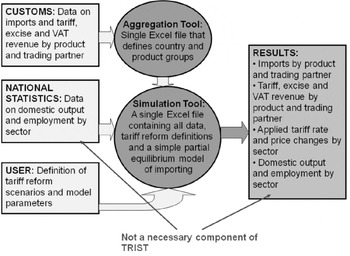
Figure 1 gives an overview of the structure of TRIST and how it works. First, the data from customs are organized within the Data Aggregation Tool and then uploaded into the Simulation Tool, within which the user defines the relevant tariff reform scenarios for each trading partner and parameterizes the elasticities of the trade model underlying TRIST, which we discuss below. A separate worksheet within the Simulation Tool presents the results of the chosen reform scenario. It illustrates the impact on tariff, excise, and VAT revenues as well as on prices at the sector level. When available, production data can be read directly into the Simulation Tool. This additional information is however not required for TRIST to function.
How TRIST works

An integral part of TRIST is the trade model that underlies the quantification of the effects of trade reform scenarios on imports, revenues, and production. The trade model in TRIST is based on four core assumptions: First, the model is derived from standard consumer demand theory and utilizes elasticities to determine the magnitude of the demand response to the price changes that result from a tariff reform.Footnote 11 Second, the calculations are based on the standard Armington (Reference Armington1969) assumption of imperfect substitution between imports from different trading partners since consumers distinguish products by the place of production. This intuitive assumption is standard in empirical international trade work and implies that a fall in the price of imports from country A relative to country B will only lead to a partial and not complete substitution of imports from country B with imports from country A.
Third, the model does not allow for direct substitution between different products. In other words, each product is modeled as a separate market and in isolation from other markets. This is perhaps the strongest assumption used in the model. However, a relaxation would not only complicate computations but would also generate a need for a range of additional ad-hoc assumptions regarding the precise design of the additional substitution effect and its parameterization. In the light of our goal to keep the model simple and transparent and to facilitate country ownership of the tool, we regard this simplifying assumption a sacrifice worth making.
Fourth, it is assumed that all changes in tariffs are fully passed on and that the world price for each product remains unchanged. That is to say that we assume an infinite supply elasticity of imports so that changes in demand in the importing country have no effect on the world price of the product; a realistic assumption for small low-income economies.
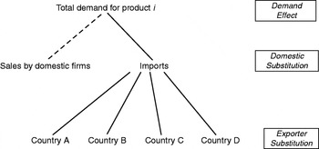
Let us now have a closer look at the three calculation steps (see Figure 2) determining the import response in our trade model.Footnote 12 In the first stage we model the allocation of given expenditure on imports of a product across different country suppliers and how this allocation changes when tariffs and duties are amended. The exporter substitution effect defines how imports from exporter A are substituted for imports from exporter B when the price of imports from exporter A relative to B declines, for example following a preferential trade reform that includes exporter A but not exporter B. The extent to which a given change in relative prices translates into a change in relative imports depends on a user-defined exporter substitution elasticity. In order to isolate the exporter substitution effect, total imports are held constant in this step.
In the second calculation step, total expenditure on a given product is allocated between domestic sources and imports. The domestic substitution effect allows for a demand shift between domestic production and imports when the relative price of imports changes.Footnote 13 The extent to which the share of imports in domestic consumption changes depends on a user-defined domestic substitution elasticity. The change in imports is then distributed across all importers according to their share of the import market. This calculation step can only be modeled if data on domestic production are available. If this is not the case, domestic substitution is not modeled and the domestic substitution elasticity becomes irrelevant.
The third and final calculation step allows for an overall demand effect in response to the change in the average price of domestic consumption of the good. The average price change is computed as an average of the price change in imports and the price change in domestic production, weighted by their relative shares in domestic consumption. A decrease/increase in the average price of the product leads to a percentage increase/decrease in overall consumption of the product, proportionately distributed between imports and domestic production. The extent to which imports change for a given change in the overall price depends on a user-defined import demand elasticity.
The trade model in TRIST

This description of the three calculation steps has outlined the crucial role played by elasticities as the parameters of the model. Elasticities are notoriously difficult to estimate, and so detailed and robust estimates of the three elasticities (exporter substitution, domestic substitution, demand) are not readily available in the literature. TRIST includes default values for each of these three parameters that are common across products and import suppliers. The sensitivity of the results can be easily assessed by changing the values of the elasticities with the option to vary them both across products and suppliers.
When detailed local knowledge on these elasticities is available, TRIST allows users to define trading partner and product-specific elasticities. Furthermore, there is an option to include the most well-known estimates of elasticities in the literature. First, the user can choose to incorporate the import demand elasticities estimated in Kee et al. (Reference Kee, Nicita and Olarreaga2004) . However, these elasticities are not available for all product groups (HS 6 digit). Second, the user can choose to use the product-specific import demand elasticities used in SMART.Footnote 14 For exporter substitution elasticities or domestic substitution elasticities, there are no estimates available at the level of product detail that TRIST uses.
4. Examples of policy issues that can be addressed in TRIST
In this section, we will give some examples of how TRIST can be used to determine the magnitude of short-term adjustment costs to tariff reform. We begin by focusing on the revenue implications and then move on to show how TRIST can be used to provide insights into the potential short-term impact of tariff reforms on domestic production and employment. In the following, we go through some examples of unilateral, bilateral, and regional trade reformsFootnote 15 that have been analyzed using TRIST.
Example 1: The COMESA customs unionFootnote 16
A pressing trade policy issue currently facing COMESA members is the impact of joining the customs union (CU). We choose three countries to analyze the revenue impact of such a scenario, Malawi, Kenya, and Zambia. The trade policy scenario is defined as follows: all the remaining non-zero intra-COMESA tariffs are set to zero. This implies assuming that a complete COMESA Free Trade Agreement (FTA) is put in place before the implementation of the customs union. Preferential tariffs with SADC members remain the same. The COMESA common external tariff (CET)Footnote 17 is applied to all remaining trading partners. However, in order to account for tariff exemptions, statutory tariffs in the CET schedule are multiplied by the current ratio of collection efficiency, i.e. the tariff revenue that has been collected divided by the revenue that should have been collected according to the current statutory rates.
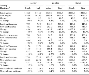
Table 2 presents results of revenue losses from the above-defined COMESA CET scenario. We choose two sets of elasticity values: the default values and higher values to assess sensitivity. In Malawi, the implementation of the CET is projected to lead to a moderate reduction in protection as the import weighted average tariff rate falls from 5.4 to 5.1%. Tariff revenues are projected to fall by US$3.6 million with the default elasticities and by US$6.6 million with the higher elasticity values corresponding to losses of between 4.8% and 8.7% of tariff revenue. Total trade revenue losses from tariffs, excises, and VAT are projected to be between US$5.2 and US$6.6 million, a fall of about 2–2.5% in overall trade tax revenues.Footnote 18 Zambia and Kenya would lose proportionately more revenue as a result of the implementation of the CET. The tariff revenue loss is predicted to be between 17% and 20% in Zambia and between 24% and 27% in Kenya. The total trade revenue loss is projected as being between 4.6% and 5% in Zambia and between 6.3% and 6.8% in Kenya.
Predicted revenue implications of a COMESA common external tariffFootnote 1 (millions of US$)

Notes: 1 The COMESA CET scenario assumes zero tariffs among COMESA partners, unchanged tariffs for SADC partners. For all other trading partners, the new CET rate is applied but deflated by the current ratio of collection efficiency (collected tariff rate / statutory tariff rate) to account for tariff exemptions. In the few cases of tariff lines for which no final agreement has been reached yet the lowest tariff rate under consideration is used.
2 The default scenario assumes 0.5 for import demand elasticity, 1.5 for exporter substitution elasticity. High scenario assumes 1 for import demand elasiticity, 5 for exporter subsitution elasticity.
Example 2: An economic partnership agreement (EPA) with the EUFootnote 19
An important challenge for many low-income countries is the negotiation and implementation of EPAs with the EU. In contrast to the previous Cotonou and Lome Agreements, these new agreements call for the reciprocal elimination of tariffs on imports from the EU. In many African, Caribbean, and Pacific countries, lack of information about the potential magnitude of the adjustment costs that will arise from removing tariffs against imports from the EU has led to considerable uncertainty and apprehension concerning these agreements.Footnote 20
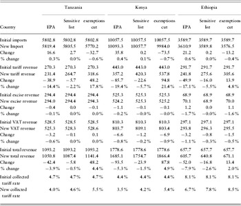
Table 3 contains simulation results for trade reform scenarios related to the implementation of the EPAs. We consider three countries for which EPAs are currently high on the policy agenda: Tanzania, Kenya, and Ethiopia. For each of the three countries, the first column of the table considers an EPA scenario in which all tariffs on products from the EU are set to zero. As discussed earlier, countries are being allowed to exclude around 20% of their imports from the EU from liberalization. The revenue losses predicted in this first exercise should thus be seen as an upper bound on the likely impact of the agreement.
Predicted revenue implications of an economic partnership agreement (EPA) with the European Union (millions of US$)

As a result of removing tariffs on imports from the EU, the average level of protection falls in all countries, with average import weighted collected tariff rates falling from 4.7% to 4.0% in Tanzania, from 4.4% to 3.5% in Kenya, and from 8.1% to 6.7% in Ethiopia. All three countries loose more than 10% of tariff revenue due to the EPA and there are overall trade tax revenue losses of 3.9% in Tanzania, 5.3% in Kenya, and 7.9% in Ethiopia.Footnote 21
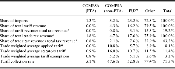
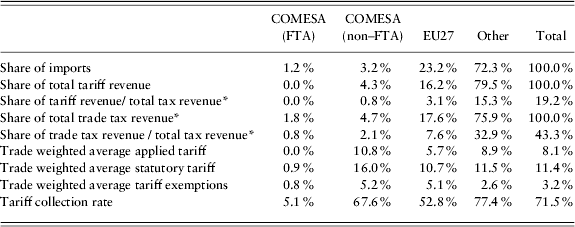
In the following, we chose Ethiopia as an example to consider the results of the simulation exercise in somewhat more detail. Table 4 presents some of the basic summary statistics for Ethiopian imports that TRIST automatically produces. The first row shows the share of each of the four main groups of import suppliers in Ethiopian imports. The EU accounts for just under a quarter of Ethiopian imports. COMESA countries, on the other hand, are relatively small suppliers of the Ethiopian market, with other countries contributing the vast majority of imports. The second row shows that the share of the EU in tariff revenue was 16.2%, and thus less than its share in imports, with the opposite being the case for imports from other countries. Tariffs on total imports account for 19% of Ethiopia's total tax revenue, with tariffs on imports from the EU contributing 3.1% of tax revenues.Footnote 22 When VAT and excise taxes levied on imports are taken into account, imports from the EU contribute 7.6% of tax revenues, while total imports provide 43.3% of revenues. Trade is clearly a key source of tax revenues in Ethiopia.
Sources of tariff revenue in Ethiopia (2005)
Note: * Based on IMF data on total tax revenue.
The trade weighted average applied tariff is 5.7% for the EU, below the overall average of 8.1%. Conversely, the tariff actually levied on imports from other COMESA countries and the rest of the world is above the overall applied average, while applied tariffs to member countries of the COMESA FTA are close to zero even though Ethiopia is not yet a member of the FTA. It should be noted that these are trade weighted tariff averages, so a higher number reflects the fact that imports are concentrated on products with a high level of protection. The tariff collection rate (the ratio of actual tariff revenue to hypothetical tariff revenue had the statutory tariff rate been applied) is 52.8% for imports from the EU, which is below the average for all imports (71.5%), and highlights the importance of taking into account exemptions when analyzing trade policy changes towards the EU.
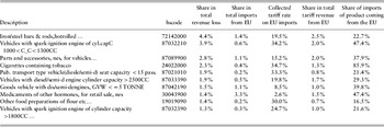
Finally, we provide more detail on the commodity and sector concentration of the estimated impacts of an EPA. Table 5 identifies the ten top tariff lines that account for the largest revenue losses following the removal of tariffs on imports from the EU (change in revenue on a given product category divided by total change in revenue). Typically, these products are characterized by a combination of relatively high imports from the EU coming in under high applied tariffs, resulting in a relatively high amount of tariff revenue collected.Footnote 23
Top ten products in terms of revenue loss from free trade with the EU

Table 5 shows that the products with the highest revenue losses typically have a medium share of imports from the EU. There is a conceptual reason for this in the trade model underlying TRIST: if imports from the EU are 0% for a product, liberalization with the EU will not lead to revenue losses. However, if the import share from the EU is 100%, all tariff revenue on these imports will be lost, but there will not be any substitution away from other exporters. Thus, in relative terms, the revenue losses per unit of EU imports are the highest if only around half of the imports of a product come from the EU. Note that these results are based on the same demand and substitution elasticities across products, thus the differences between products are not driven by the value of elasticities.
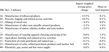
Table 6 aggregates the estimated changes in prices at the ISIC (International Standard Industrial Classification) Rev. 3 industry level to obtain industry level changes in overall import prices. These figures give an indication of the sectors that are likely to face the stiffest increase in competition as tariffs on the EU are removed. For Ethiopia, import prices for tobacco products and forestry products fall by around 15%. For all other sectors, the competition effect is likely to be milder with price changes of imports of less than 5%.
Ethiopian import price changes by sector under EPA scenario

As mentioned previously, countries often negotiate to exclude particular products from tariff removal commitments. In TRIST, any user-defined list of products can be selected to be excluded from the EPA or any other trade agreement since the model is based on data at the tariff line level. As an example, we look at the case in which countries choose the exclusion list to minimize the adverse revenue impact on the agreement. In TRIST, we can simply run the EPA scenario without an exclusion list and then rank products by the ratio of overall trade tax revenue loss to import value from the EU. We then select the sensitive products beginning with those that have the highest ratio until we reach a cumulative share of 20% of imports from the EU.
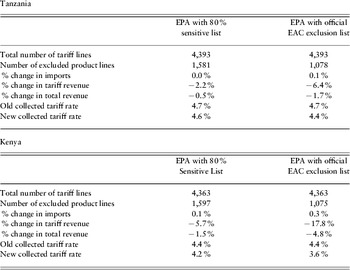
The results from this scenario are presented in the second column of Table 3 and show that the fall in tariff revenues compared to the initial EPA scenario without the exclusion list is considerably reduced by between 12 and 14 percentage points for the three countries. The overall trade tax losses under this scenario amount to 0.5% (Tanzania), 1.5% (Kenya), and 2.6% (Ethiopia). For some countries, official exclusion lists for a potential EPA have already been determined. Among these are the EAC (East African Community) member states Tanzania and Kenya. Table 7 contrasts the impact of an EPA under the revenue loss minimizing scenario outlined in column two of Table 3 with a scenario in which the official EAC exclusion list is used. In the case of Tanzania, the projected 1.5% loss in trade tax revenue is only slightly higher than the losses projected for the revenue loss minimization case, whereas revenue losses for Kenya are closer to the projected impact for an EPA without an exclusion list. This indicates that the EAC exclusion list may have been determined to respond more closely to Tanzanian rather than Kenyan revenue concerns.
Tanzanian and Kenyan EPA with official EAC exclusion list

Another policy response to declining tariff revenues due to trade liberalization is the removal of tariff exemptions. In Table 3, the third column presents the impact of a scenario in which all tariffs with the EU are set to zero, with no exclusion list, and tariff exemptions are cut to zero. All three countries gain substantial amounts of tariff and overall trade tax revenue by cutting exemptions despite the fact that all tariffs with the EU are set to zero. Similarly, in all three countries the reform actually leads to an increase (of between 2% and 4%) rather than a decrease in import weighted average collected tariffs. However, the removal of tariff exemptions could exacerbate the negative, trade diverting, impact of the preferential trade agreement. It is important that a country also seeks to reduce its MFN (most favoured nation) tariffs to reduce the possible distortions that arise from removing tariffs against particular suppliers and not others. Hence a commitment to reduce tariffs against the EU should be coordinated with the removal of tariff exemptions. For example, removing all tariff exemptions would allow Tanzania to cut its MFN tariffs by more than 30% at the same time as implementing the EPA agreement without any adverse revenue impact. Similarly, Ethiopia could cut its MFN tariffs by more than 20% and Kenya by more than 40%.
Example 3: ‘Trade diversion’ and ‘trade correction’Footnote 24
A preferential tariff liberalization will reduce prices of imports from the beneficiary country. This creates a potential for trade diversion if the good is produced less efficiently in the preferred source than in countries subject to the full tariff. The topic of trade creation vs. trade diversion, and the resulting welfare implications, is well-known, and can be addressed in TRIST in a standard way similar to existing tools like SMART with the help of an easy to install add-on tool.
However, TRIST adds an additional dimension to this type of analysis by also looking at what can be referred to as trade correction: the reversal of previous trade diversion. Consider the following example: after the EU is granted tariff free market access, it takes over some of the market share that was previously held by other trading partners who already enjoyed tariff free market access prior to the EU being granted the tariff reduction. This would not be trade diversion as it would actually imply a move of consumption towards a more efficient producer that was previously disadvantaged in terms of market access.
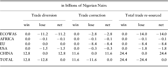
As a practical example, we consider a sequential scenario: we assume that Nigeria has liberalized all tariffs on imports from the EU to zero as part of an EPA. The resulting import allocations and tariff rates are taken as the ‘base scenario’ for the following policy experiment, namely an FTA between Nigeria and China. Table 8 shows how different trading partners would be affected in terms of their exports to Nigeria if Nigerian tariffs on all Chinese imports were preferentially driven to zero as part of the FTA. The table distinguishes two categories of re-sourced trade as outlined above: diverted trade that is welfare reducing (trade diversion) and changes in response to a decrease in preferences previously granted which is not welfare reducing (trade correction).
Trade diversion vs. trade correction for a Nigerian FTA with China
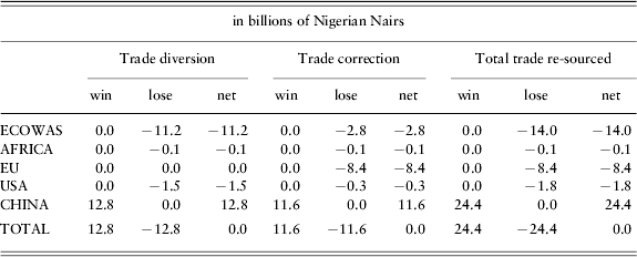
Table 8 shows that Nigeria now imports an additional 24.4 billion Naira worth of goods from China. Imports from all other trading partners decline, with trade diverted away from the EU being entirely due to trade correction. The reason is that imports from China increase at the expense of EU goods in product categories in which Chinese exports were initially disadvantaged by preferences given to EU exports under the EPA. For all other partners some of the decline in exports to Nigeria is classified as trade diversion and some is classified as trade correction. This is because some, but not all Chinese products had initially been subject to significant discrimination from preferences given to other trading partners.
Example 4: The impact of specific and complex dutiesFootnote 25
TRIST can also deal effectively with specific and complex tariffs. Specific tariffs are those in which the duty is related to the volume or other physical characteristics of the product rather than its value, while complex tariffs combine different types of duties such as ad valorem and specific tariffs. A key feature of specific and complex tariffs is that the level of protection given by the statutory rate is not transparent and in practice will vary across different transactions of the same product. These tariffs tend to be regressive since higher proportional rates of protection are applied to the lower value transactions that are consumed by poor households. Footwear is a good example of a product that is often subject to specific duties – often a fixed amount per pair. In Mauritius, for example, in 2007 there was a specific duty of 125 rupees per pair on certain types of footwear with uppers of leather and outer soles of rubber, plastics, leather, or composition leather. The ad valorem impact of such a fixed tax will be much greater on relatively cheap shoes from India than on a pair of Jimmy Choo's! Indeed, the data in TRIST show that in 2007, the ad valorem equivalent tariff on imports of such footwear from India (39.8%) was more than double that on imports from the EU (19.2%), while the ad valorem equivalent tariff on the small quantity of imports from Italy was 9.4%.
The data in TRIST are based on actual revenues collected and so TRIST automatically computes ad-valorem equivalents of specific and complex tariffs for each product by country import flow. Hence, TRIST can show the revenue and other adjustment implications of removing specific and complex tariffs or of strategies to convert them into ad valorem rates. Other tools that are based on statutory rates rather than collected revenues use formulas to calculate approximate ad valorem equivalents. For example, in WITS (World Integrated Trade Solution), for simple specific tariffs, the ad valorem equivalent is calculated by dividing the specific duty by the unit value (value divided by quantity). The unit value is based either on the importing countries total imports of the product from the world or the global imports of OECD countries (Stawowy, Reference Stawowy2001). The use of these more aggregated unit values reflects concerns with the quality of the information on the quantity of individual import flows. However, there remain many gaps in the WITS database regarding ad valorem equivalents of specific duties. For example, in WITS, the duties levied by Mauritius on leather footwear are reported as zero whichever method of calculation is used.
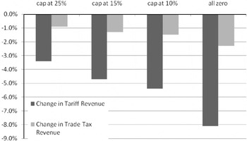
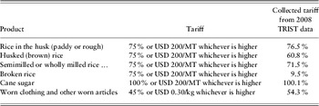
Table 9 shows statutory complex tariffs in the Tanzanian tariff schedule and Figure 3 illustrates the revenue implications of converting them to ad-valorem equivalents and subsequently reducing these. Again, there is an important difference in the projected changes in tariff revenues and changes in total import tax revenues, with the percentage change in the former being around four times greater than that of the latter. The contribution of such taxes to trade revenues is relatively small, such that conversion to an ad valorem rate of 25% (the maximum rate in the common external tariff of the East African Community) would lead to import tax revenue losses of less than 1%. Complete abolition of these duties would result in trade revenue losses in the order of 2%. These losses would need to be judged relative to the distortion of trade created by these duties, their regressive impact on poor households, and the additional administrative costs for customs in applying them relative to ad valorem duties.Footnote 27
Revenue implications of replacing specific with ad-valorem tariffs in Tanzania

Specific tariffs in TanzaniaFootnote 26

Example 5: The impact of trade reforms on output and employment
Up to this point, this paper has focused on the analysis of revenue changes in response to trade policy reforms. Yet, revenue effects are not the only adjustment cost policy makers may need to address. The following analysis shows how TRIST can be extended to provide input to an analysis of the short-term impact of trade reforms on domestic production and employment.
However, again, it is important to note that TRIST uses a partial equilibrium model and thus does not take into account inter- and intra-sectoral linkages and the economy-wide impacts of tariff changes. The results presented below are based on tariff line level partial equilibrium simulations which do not take into account the various economy-wide resource constraints and reallocations, or any inter- and intra-sectoral economic linkages that may be important for the medium- to long-term impacts of the respective reforms. One of the core benefits of trade liberalization is that it removes the anti export bias in economies with high levels of protection which will depreciate the real exchange rate and allow export sectors to compete more effectively for domestic factors of production. This not only implies that export intensive sectors might benefit disproportionately from trade liberalization and are likely to expand in the medium to long term, but also that an assessment of the short-term aggregate impact of a liberalization scenario on domestic production may be subject to a systematic upward bias.Footnote 28
These concerns are less of an issue with respect to relative sectoral impacts of tariff reform. Given its nature as a partial equilibrium model, the purpose of TRIST in contributing to the analysis of trade reform adjustment costs in terms of output and employment is thus to identify sectors that are likely to be hardest hit as part of the direct short-term adjustment to increased competition in import markets, to assess the magnitude of these differences, and to contribute to the design of policy interventions that seek to cushion these direct adjustment costs.Footnote 29
The impact of trade reforms on domestic production, and in particular on employment, has been one of the most politically sensitive issues in the discussion on adjustment costs. In the long run, trade liberalization leads to the reallocation of production factors (labor and capital) to more productive uses, and thus changes in the pattern of production and employment among and within firms, industries, and regions. In the short run, production in import competing sectors will tend to decline, which may have social and political costs. A better understanding of these effects is central to effective sector- and region-specific trade policy making that mitigates these adjustment costs.
A first indication of those sectors that are likely to be most affected by short-term adjustment costs to tariff reform can be gained by looking at changes in prices for each sector. These will be larger for sectors where average tariffs fall the furthest. However, this analysis can be considerably enhanced and deepened if there are detailed data at the sector level on domestic sales (production minus exports) and employment. These can be uploaded into the Simulation Tool and TRIST will automatically amend the model to include the domestic substitution effect as well as present sectoral changes in domestic production and employment that result from the tariff reform scenario of interest. The short-term impact of a tariff reform on output and employment will be determined by the size of the change in the tariff at the sector level, the short-run elasticity of supply, and the initial size of the sector. The exercise will show that large sectors facing significant tariff reductions are likely to face the greatest adjustment in the short term.Footnote 30
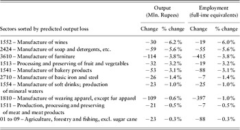
A country for which a TRIST has been developed and for which the necessary data on sectoral domestic production (at the 4-digit level) are available is Mauritius. Table 10 presents selected results illustrating the impact of a duty-free island trade policy scenario on output and employment. The move towards a tariff free island reduces the share of output directed towards the domestic market because of higher competition from imports. Employment results are based on the assumption that the number of full-time equivalent jobs in companies declines proportionately with output. We do, however, control for the fact that in some sectors – especially textiles and wearing apparel – production for the domestic market is more labor intensive than export oriented production.Footnote 31 The table presents changes in domestic production and employment in the ten sectors that are projected to be most severely affected (in terms of output losses) by the reform scenario. These are the manufacture of furniture, wearing apparel, soap and detergents, bakery products, preserving of fruits and vegetables, and wine.
Duty-free island in Mauritius: 15 most affected sectorsFootnote 32

The results suggest that short-run employment adjustments are likely to be concentrated on two sectors, with more than three-quarters of the projected loss of employment occurring in furniture and apparel. This analysis supported the government in introducing a program to assist adjustment of the furniture sector.
5. Conclusions
TRIST is a simple, easy to use country focused model that brings substantial advantages in simulating the impact of trade reforms and thus in evaluating different trade policy options. It contributes to a better understanding of trade-related adjustment implications which is crucial to design a reform agenda that maximizes benefits from greater openness while minimizing and adequately cushioning adjustment costs. While TRIST has been developed to simulate the short-term implications of trade reform on fiscal revenue, TRIST can be extended to estimate the differences between trade creation, diversion, and correction with the resulting welfare implications as well as the initial impact of trade reform on domestic production and employment in import competing sectors.
The key features of TRIST compared to previous studies and models are that it uses collected tariff rates at the tariff line level, which leads to greater accuracy than using statutory rates; it takes into account all taxes collected levied on trade, not only tariff revenue, but also revenue from VAT and excise taxes; it works at a highly disaggregated and policy relevant level, breaking down results for detailed products and trading partners; it is transparent, open, and flexible and does not require sophisticated software or specific programming skills. The overarching goal of TRIST is to provide a tool to government agencies and other stakeholders that can use it to support an informed discussion of the possible short-term consequences of tariff reforms.
It is hoped that free access to the spreadsheet tool will allow researchers and government officials to fine tune TRIST to reflect country circumstances, and will enable them to analyze the impact of proposals for trade policy reform as they arise. An aim of this paper and tool is also to encourage the collection of more accurate and detailed data on production, employment, and consumption. This is important to allow for more systematic analysis of the impact of trade (and other) policy changes on output, employment, consumption, and poverty so as to help motivate positive interventions that limit the adjustment costs, and so maximize the overall positive economic benefits, of trade reform.
TRIST templates as well as a TRIST manual, additional information, and links to publications using TRIST are available at http://go.worldbank.org/2P8FPC0760.
Appendix: Detailing the calculation steps in the trade model
The trade response to a change in tariffs for a given product from a given exporter is calculated based on the resulting percentage change in the duty inclusive price. It is assumed that all changes in tariffs are fully passed on and that the world price remains unchanged (infinite supply elasticity). For a change in the tariff (with VAT and excise rates unchanged), the percentage change in the price of good i from exporter j is calculated as follows (subscript i is omitted for all arguments in the formula)

where
Δp j is the change in price of imports from country j,
p jold is the price of imports from j before tariff reform,
p jnew is the price of imports from j after tariff reform,
p wld is the world market price,
t jold is the tariff rate applied to imports from country j before reform,
t jnew is the tariff rate applied to imports from country j after reform,
ext j is the excise tax rate applied to imports from j, and
vat j is the VAT rate applied to imports from j.
The trade response for a particular product is modeled in three consecutive steps. In the first stage, we model the allocation of given expenditure on imports of a product across different country suppliers and how this allocation changes when tariffs and duties are amended. To isolate this substitution effect, total imports are held constant (product subscript i is omitted for all arguments in the formula)
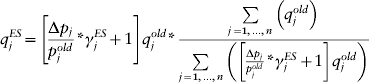
Where q jES is the imported quantity from j after exporter substitution step,
q jold is the imported quantity from j before reform, and
γjES is the exporter substitution elasticity for imports from country j.
In the second step, total expenditure on the product is allocated between domestic sources and imports. The change in imports resulting from this step is then distributed across all importers according to their share of the import market. By definition total domestic consumption remains constant in this stage
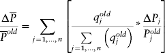
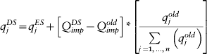
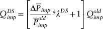
where
Q impold is the initial total imported quantity,
Q impDS is the total imported quantity after substitution with domestic output,
q jDS is the quantity imported from supplier j after substitution between imports and domestic output,
λDS is the domestic substitution elasticity for imports from exporter j, and
 is the change in price of total imports.
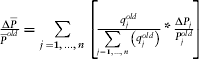 is the change in price of total imports.
In the third and final step, the demand effect, the change in the price of imports leads to an overall change in the price of the product (given by the change in the aggregate price of imports weighted by the share of imports in domestic consumption), which in turn results in a change in domestic consumption of a good. The additional consumption resulting from this effect is distributed across both imports and domestic production according to initial shares of total consumption of the product.
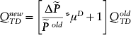

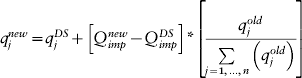
where Q TDold is the initial total demand for product I,
Q TDnew is the total demand after the change in the overall price of product I,
Q domoldis the initial quantity of demand for domestic output,
Q domnewis the final demand for domestic output
Q impnewis the final demand for imports of product I,
q jnew is the quantity imported from supplier j after all three effects from changes in import prices (the substitution between different sources of imports, between imports and domestic output, and the demand effect for the product as a whole),
μD is the demand elasticity for product I, and
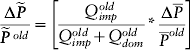
is the change in the price of total domestic consumption.