NOMENCLATURE
- MAV
Micro-Air-Vehicle
- LEV
Leading Edge Vortex
- UVLM
Unsteady Vortex Lattice Method
- CFD
Computational Fluid Dynamics
- LE,TE
Leading edge, trailing edge
- LEV
Leading edge vortex
- SS4
Model skill score
- QS
Quasi-Steady
Symbol
 $\mathcal{O}(\cdot)$
Order of magnitude
-
$\mathcal{E}$
,
$\partial\mathcal{E}$
,
$\mathcal{C}$
,
$\partial\mathcal{C}$
Set of points within and at the boundary of an elliptical and circular cross-sectional shaped body, respectively
-
${\boldsymbol{\omega}}$
,
$\omega$
Angular velocity and its magnitude, respectively
-
$\hat{\textbf{\textit{n}}}_1, \hat{\textbf{\textit{n}}}_2, \hat{\textbf{\textit{n}}}_3$
Orthonormal set of unit vectors defining an inertial reference frame
-
$\hat{\boldsymbol{e}}_1, \hat{\boldsymbol{e}}_2, \hat{\boldsymbol{e}}_3$
Orthonormal set of unit vectors defining a body-fixed reference frame
- O
Pivot point of the wing section
- t
Time
-
${\textbf{\textit{r}}}$
Position vector
-
${\textbf{\textit{v}}}({\textbf{\textit{r}}}_p,t)$
Velocity of an arbitrary point P within the body
-
${\textbf{\textit{u}}}({\textbf{\textit{r}}},t)$
Fluid velocity at location
${\textbf{\textit{r}}}$
-
${\textbf{\textit{r}}}^{P/O}$
,
${\textbf{\textit{r}}}^{C/O}$
Relative position of points P and C, respectively, with respect to point O
-
${\textbf{\textit{r}}}^{O/C}$
,
$z_O$
Relative position of point O with respect to point C, and its complex counterpart, respectively
-
${\textbf{\textit{v}}}_O$
,
$V_O$
Velocity of point O and its magnitude, respectively
-
${\textbf{\textit{v}}}_C$
,
$\mathscr{V}_C$
Velocity of point C and its complex counterpart, respectively
-
${\textbf{\textit{u}}}_\infty$
,
$U_\infty$
Velocity of the free flow and its magnitude, respectively
-
$\varphi$
,
$\vartheta$
Orientation of the
${\textbf{\textit{v}}}_C$
and
${\textbf{\textit{u}}}_\infty$
with respect to
$\hat{\textbf{\textit{b}}}_1$
, respectively-
$\hat{\textbf{\textit{s}}}_\varphi$
,
$\hat{\textbf{\textit{s}}}_\vartheta$
Unit vectors defining the direction of
${\textbf{\textit{v}}}_C$
and
${\textbf{\textit{u}}}_\infty$
, respectively-
$\Phi$
Velocity Potential
-
$\hat{\textbf{\textit{n}}}({\textbf{\textit{r}}})$
Unit vector normal to the surface of the body
$\mathcal{E}$
at location
${\textbf{\textit{r}}}$
-
$p({\textbf{\textit{r}}})$
,
$p_\infty$
Pressure at location
${\textbf{\textit{r}}}$
and at infinity, respectively-
$\rho$
Fluid density
-
$g(\cdot)$
Conformal map
-
$\lambda$
Conformal map parameter
- j
Imaginary unit
-
$\zeta, z$
Complex coordinates in the circle and physical plane, respectively, defined in the body-fixed frame
-
$\mathscr{F}$
Complex potential
-
$\Gamma$
,
$\Gamma_j$
Point vortex intensity
-
$\mu_j$
,
$\beta_j$
Doublet intensity and orientation, respectively
- R
Circle radius
-
$\mathcal{F}$
Complex force
-
${\textbf{\textit{F}}}$
,
${\textbf{\textit{F}}}_{\text{2D}}$
,
${\textbf{\textit{F}}}_{\text{3D}}$
Vector force per se, two-dimensional, and three-dimensional, respectively
-
${\textbf{\textit{F}}}_{\text{LE}}$
,
${\textbf{\textit{F}}}_{\text{LEV}}$
Leading edge force, Leading edge vortex force
-
$\varrho$
Leading edge vortex force parameter
-
$\gamma_\mathcal{E}$
,
$\gamma_\mathcal{W}$
Vortex sheet intensity distribution
-
$A_{ij}$
Influence coefficient of vortex j over control point i
-
$C_{d\_{qs}}$
,
$C_{l\_{qs}}$
Quasi-steady translation drag and lift coefficient
-
$\alpha$
Flat plate angle-of-attack
-
$t_vV/c$
Nondimensional time for computation of quasi-steady translation loads
-
$C_d$
,
$C_l$
Normalised drag and lift coefficient
-
$A_f$
,
$\Theta$
Amplitude of the translational and rotational motion, respectively
- b,
$\mathcal{S}$
Wing span and planform area of a three-dimensional planar wing
-
$r_{11}$
Radius of gyration abut the axis along the
$\hat{\textbf{\textit{e}}}_1$
direction


1.0 INTRODUCTION
Over the last three decades, considerable research efforts have been made towards understanding the basis of insect and bird flight. Although initially stemming from a biological perspective, these efforts have received additional motivation from the field of micro-air-vehicles (MAVs). Flapping-wing animals and insects became a source of inspiration (bioinspiration) for the design of small flying vehicles. Thus, understanding the aerodynamics of flapping wings is important to aid the engineering of highly manoeuverable and stable flapping-wings flying devices. A thorough review of flapping-wing aerodynamics for insects and vertebrates, highlighting their similarities and differences has been provided by Chin and Lentink(Reference Chin and Lentink1). Shyy et al(Reference Shyy, Kang, Chirarattananon, Ravi and Liu2) have reviewed recent advances in insect-scale flapping-wing aerodynamics, flexible wing structures, unsteady flight environment, sensing, stability, and control.
Unsteady aerodynamic mechanisms of flapping wings were first explained by Weis-Fogh(Reference Weis-Fogh3), and later analysed in a series of works by Ellington(Reference Ellington4). There is a general agreement amongst the numerous studies conducted to date that hovering birds and insects increase lift through the so-called delayed stall mechanism(Reference Dickinson and Götz5). This mechanism is based on the generation of a stable leading edge vortex (LEV) that remains close to the leeward side of the wing during the stroke only to be shed at the end of it. This “attached vortex” reduces the pressure on the back of the wing, an effect analogous to that of spiral delta wing tip vortices. The stability of this growing vortex was conjectured to be due to the axial flow along the wing span(Reference Birch and Dickinson6). Other mechanisms of lift enhancement are wake capture(Reference Dickinson, Lehmann and Sane7,Reference Birch and Dickinson8) , rotational circulation(Reference Dickinson, Lehmann and Sane7,Reference Sane9) akin to the so-called Magnus’ effect, and clap and fling(Reference Weis-Fogh3) employed by tiny insects. It has also been proposed by several researchers that the flexibility of the wing increase the lift-to-drag ratio(Reference Vanella, Fitzgerald, Preidikman, Balaras and Balachandran10,Reference Fitzgerald, Valdez, Vanella, Balaras and Balachandran11) .
The objective of this article is to provide a thorough comparison between several modeling approaches and experimental data available in the literature on flapping-wing aerodynamic loads. The two approaches considered, from which different variants stem, are of analytical and computational nature. In the analytical approach, whose baseline is the potential flow theory, the resultant force is obtained through a novel generalisation of the leading edge suction analogy. The computational approach is based on the Unsteady Vortex Lattice Method (UVLM), which although stemming from the potential flow theory, includes a wake model and hence, allows one to account for the wake’s effect on the aerodynamic loads. The same leading edge suction analogy generalisation is used in this approach to modify the predicted forces. The models are two-dimensional in nature but could be extended to three dimensions by means of the blade-element theory.
1.1 Brief review of past related research
Sane(Reference Sane9), and Ansari et al(Reference Ansari and Knowles12) have reviewed some of the methodologies employed to study insect flight mechanisms. Amongst the inviscid classical methods, it is worth noting the blade-element and the actuator disk theories(Reference Weis-Fogh13, Reference Jensen14, Reference Ellington4), the thin airfoil theory(Reference DeLaurier15), and the lifting-line and lifting-surface methods(Reference Betteridge and Archer16).
Several other analytical inviscid methods have been developed. For instance, Minotti(Reference Minotti17) presented a two-dimensional analytical model with the leading edge and trailing edge flow separations accounted for by two vortices at a fixed location with respect to the wing section. Żbikowski(Reference Żbikowski18) outlined two analytical approaches to study the aerodynamics of insect-like flapping wings in hover, one based on circulation and the other based on the velocity potential. Following those lines, Pedersen and Żbikowski(Reference Pedersen and Żbikowski19) combined indicial methods of unsteady aerodynamics with Polhamus’ leading edge suction analogy and accounted for wake effects through the analytical solutions of Wagner, Küsner, and Loewy. Also, Ansari et al(Reference Ansari, Żbikowski and Knowles20,Reference Ansari, Żbikowski and Knowles21) presented an analytical model based on the circulation method and conformal mapping. A discrete vortex method was used to obtain numerical solutions of the derived equations. Finally, Yu et al(Reference Yu, Tong and Ma22) used a continuous distribution of sources and sinks on the surface of a conformably transformed two-dimensional plate and free vortices to model the wakes shed from the leading and trailing edges. The Kutta condition at both edges determined the rate circulation shed off each edge.
Further progress have been made possible through CFD models of various levels of complexity. Smith et al(Reference Smith, Wilkin and Williams23) reported three-dimensional simulations of a full insect with an unsteady aerodynamic panel method employing sources and doublets on the wing and body, and doublets in the wakes. Wang et al(Reference Wang, Birch and Dickinson24) conducted CFD simulations of a two-dimensional flapping wing section with simplified kinematics and compared the results obtained with experiments and a quasi-steady theory. These researchers found that the fluid forces are mainly dominated by pressure. Liu et al(Reference Liu, Ellington, Kawachi, Van Den Berg and Willmott25) simulated the wing motion of a hovering Hawkmoth and Sun and Tang(Reference Sun and Tang26) and Ramamurti and Sandberg(Reference Ramamurti and Sandberg27) simulated the motion of a Drosophila wing. The latter found that viscosity has a minimal effect on the forces, which are mostly dominated by translation and rotational mechanisms. Nakata et al(Reference Nakata, Liu, Tanaka, Nishihashi, Wang and Sato28) developed a 12cm-wingspan hummingbird-inspired MAV and analyzed the aerodynamics of the MAV’s flexible wings through CFD and wind tunnel experiments, with emphasis on the vortex and wake structures and their relationships with aerodynamic force generation. Finally, Nakata et al(Reference Nakata, Liu and Bomphrey29) proposed a quasi-steady model, in which it is assumed that the aerodynamic forces on a flapping wing can be decomposed into quasi-steady forces and parameterised by using CFD results.
Regarding experimental studies, it is worth mentioning the robofly experiments conducted by Dickinson and colleagues(Reference Birch and Dickinson6, Reference Dickinson, Lehmann and Sane7, Reference Birch and Dickinson8, Reference Sane9, Reference Wang, Birch and Dickinson24).
2.0 MATERIALS, METHODS AND THEORY
Insects and small birds fly at low-to-moderate chord based Reynolds numbers:  $\mathcal{O}(10^1)$
for small insects such as Chalcid wasps,
 $\mathcal{O}(10^2)$
for fruit flies,
 $\mathcal{O}(10^3)$
for bees and dragonflies, and
 $\mathcal{O}(10^4)$
for moths and hummingbirds (Table 1.1, p. 15 of ref. (Reference Altenbuchner and Hubbard30)). Experimental evidence(Reference Dickinson, Lehmann and Sane7,Reference Wang, Birch and Dickinson24) has shown that the aerodynamic forces generated by flapping wings are dominated by pressure and that the viscous effects play a secondary role, even for Reynolds numbers as low as 75. Hence, the observed aerodynamic forces are primarily normal to the solid surfaces. These observations support the hypothesis that the main features of the flow and forces generated by a flapping wing can be described to certain extent through inviscid fluid models.
The system considered is a two-dimensional wing section undergoing flapping-like motions (translation and rotation) within still or moving air. In general, the wing section has an elliptical shape, which can degenerate to flat plate. Only the flat plate section is studied in this article. The resulting airflow is assumed to be incompressible and irrotational except at the interface (vortex sheet) between the solid surfaces and the air where infinitesimally thin boundary layers are present.
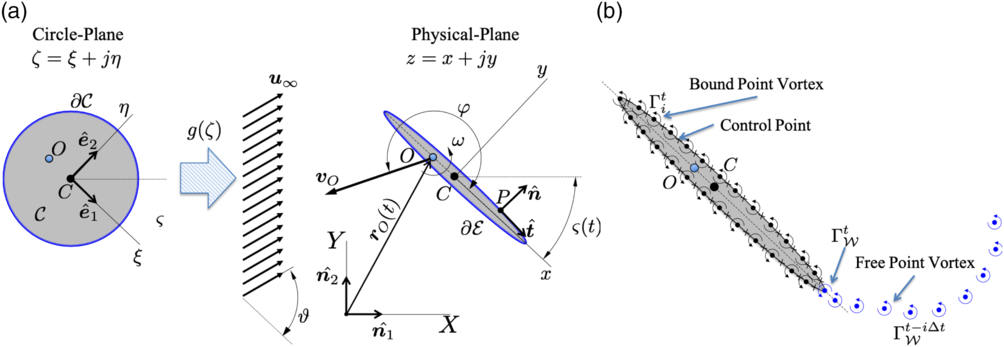
Two-dimensional elliptic body  $\mathcal{E}$
undergoing prescribed translation and rotation. (a) Conformal map of a circle into an ellipse. (b) ULVM discretization.

The motion of a body  $\mathcal{E}$
in the x-y plane is described by an angular velocity
 $\boldsymbol{\omega}=\omega\hat{\textbf{\textit{n}}}_3$
about a pivot point O and a translation velocity
 ${{\textbf{\textit{v}}}_O=V_O \hat{\textbf{\textit{s}}}_\varphi}$
of point O, with
 $\hat{\textbf{\textit{s}}}_\varphi$
a unit vector with direction given by the angle
 $\varphi$
(Fig. 1(a)). The fluid (air) may have a uniform velocity
 ${\textbf{\textit{u}}}_\infty =U_\infty \hat{\textbf{\textit{s}}}_\vartheta$
, with
 $\hat{\textbf{\textit{s}}}_\vartheta$
a unit vector with direction given by the angle
 $\vartheta$
. The velocity of an arbitrary point
 $P \in\mathcal{E}$
of the body is given by:
 \begin{align}{\textbf{\textit{v}}}({\textbf{\textit{r}}}_P,t)= {\textbf{\textit{v}}}_O+ \boldsymbol{\omega} \times{\textbf{\textit{r}}}^{P/O},\end{align}
where  ${\textbf{\textit{r}}}^{P/O}$
is the relative position of point P with respect to O. Of particular interest is the velocity of the centroid of the section C, which according to (1) is given by:
 \begin{align}{\textbf{\textit{v}}}_C(t):={\textbf{\textit{v}}}({\textbf{\textit{r}}}_C,t)= {\textbf{\textit{v}}}_O+ \boldsymbol{\omega} \times{\textbf{\textit{r}}}^{C/O}={\textbf{\textit{v}}}_O- \boldsymbol{\omega} \times{\textbf{\textit{r}}}^{O/C}.\end{align}
Assuming that the flow is irrotational outside the vortex sheets, the continuity equation for irrotational and incompressible flows becomes the Laplace Equation (3) for the velocity potential  $\Phi$
:
 \begin{align}\nabla^2 \Phi =0.\end{align}
The flow field  ${\textbf{\textit{u}}}({\textbf{\textit{r}}},t)=\nabla \Phi$
must satisfy the no-penetration condition on the surface of the body
 $\partial \mathcal{E}$
:
 \begin{align}\left({\textbf{\textit{u}}}({\textbf{\textit{r}}},t) - {\textbf{\textit{v}}}({\textbf{\textit{r}}},t)\right)\cdot\hat{\textbf{\textit{n}}}({\textbf{\textit{r}}}) = 0&& \forall\ t\in[0,\infty);\ {\textbf{\textit{r}}}\in\partial \mathcal{E}.\end{align}
Here  $\hat{\textbf{\textit{n}}}({\textbf{\textit{r}}})$
is the unit vector normal to the surface of the body at point
 ${\textbf{\textit{r}}}\in\partial\mathcal{E}$
. Additionally, it is required that the perturbations introduced by the body decay to zero far away from it. This regularity condition at infinity is satisfied by the fundamental solutions (vortex, source/sink, dipole) of the Laplace Equation (3). For incompressible, irrotational flows, the unsteady Bernoulli’s equation is employed to obtain the pressure distribution over the body surface once the velocity potential
 $\Phi$
is known. This equation is given by
 \begin{align}p({\textbf{\textit{r}}},t)-p_\infty=&\frac{\rho}{2}\left({\textbf{\textit{u}}}_\infty\cdot{\textbf{\textit{u}}}_\infty-{\textbf{\textit{u}}}({\textbf{\textit{r}}},t)\cdot{\textbf{\textit{u}}}({\textbf{\textit{r}}},t)\right)-\frac{\partial}{\partial t}\left(\Phi({\textbf{\textit{r}}},t)-\Phi_\infty\right)\ \ \text{for}\ {\textbf{\textit{r}}}\in \partial\mathcal{E}.\end{align}
2.1 Analytical potential flow formulation
The circulatory flow around a moving body  $\mathcal{E}$
is obtained through conformal mapping of the equivalent flow around a moving circle
 $\mathcal{C}$
(Fig. 1(a)). A Joukouwsky transformation
 ${g:\mathbb{C}\ni \zeta\mapsto z\in \mathbb{C}}$
(
 ${z=x+jy}$
,
 ${\zeta=\xi+j\eta}$
) is employed to transform the fluid domain outside a circle
 $\mathcal{C}$
of radius R (defined in the
 $\zeta$
-complex plane) into the fluid domain outside an elliptical body
 $\mathcal{E}$
(defined in the z-complex plane). This conformal map is given by:
 \begin{align}g(\zeta):=a\left(\zeta+\frac{\lambda^2}{\zeta}\right).\end{align}
The coordinates x-y are referred to a reference frame  $\left\{\hat{\textbf{\textit{e}}}_1,\hat{\textbf{\textit{e}}}_2\right\}$
which is attached to the centroid C of the body
 $\mathcal{E}$
. Similarly, the coordinate system
 $\zeta \hbox{-} \eta$
is referred to the frame
 $\left\{\hat{\textbf{\textit{e}}}_1,\hat{\textbf{\textit{e}}}_2\right\}$
and its origin is located at the centroid C of the circle
 $\mathcal{C}$
.
It can be shown that the complex potential  $\mathscr{F}$
of the equivalent flow around the circle
 $\mathcal{C}$
is given by:
 \begin{align}\mathscr{F}(\zeta,t){}={}& U_\infty(t) g(\zeta) e^{-j\vartheta(t)}-j\frac{\Gamma(t)}{2\pi} \ln\left(\frac{\zeta}{R}\right)-\frac{\mu_1(t)}{2\pi}\frac{e^{\,j\beta_1(t)}}{\zeta}-\frac{\mu_2(t)}{2\pi}\frac{e^{\,j\beta_2(t)}}{\zeta}\nonumber\\
&+\frac{1}{\zeta}a\left(\lambda^2\bar{\mathscr{V}}_C(t)-R^2\mathscr{V}_C(t)\right)-j\omega(t) \frac{\lambda^2a^2R^2}{\zeta^2},\end{align}
where the point vortex circulation  $\Gamma$
is taken positive in the counter-clockwise sense, the overline indicates complex conjugation,
 $\mu_1e^{\,j\beta_1}$
and
 $\mu_2e^{\,j\beta_2}$
are two dipoles defined in the
 $\zeta$
-plane and centered at C,
 $\mathscr{V}_C\in\mathbb{C}$
is the complex counterpart of
 ${\textbf{\textit{v}}}_C$
(Equation (2)) such that
 ${\textbf{\textit{v}}}_C=\mathscr{V}_C\hat{\textbf{\textit{e}}}_1$
Footnote 1. If
 $\mathscr{V}_O=V_Oe^{\,j\varphi}\in\mathbb{C}$
and
 $z_O\in \mathbb{C}$
are the complex counter parts of
 ${\textbf{\textit{v}}}_O$
(
 $=\mathscr{V}_O\hat{\textbf{\textit{e}}}_1$
) and
 ${\textbf{\textit{r}}}^{O/C}$
(
 $=z_O\hat{\textbf{\textit{e}}}_1$
), respectively, then it can be shown that
 \begin{align}{\textbf{\textit{v}}}_C=\mathscr{V}_C\hat{\textbf{\textit{e}}}_1=\left(\mathscr{V}_O-j\omega z_O\right)\hat{\textbf{\textit{e}}}_1.\end{align}
The last two terms in Equation (7), related to the body kinematics, arise from the boundary function introduced by Milne-Thompson(Reference Milne-Thompson31) (Section 9.63). It can be shown that the no-penetration Equation (4) on the circle yields:
 \begin{align}\mu_1e^{\,j\beta_1}&= -2\pi aR^2 U_\infty e^{\,j\vartheta}\nonumber\\\mu_2e^{\,j\beta_2}&=2\pi a\lambda^2 U_\infty e^{-j\vartheta}.\end{align}
2.1.1 Fluid force
The resultant (complex) force  $\mathcal{F}$
is obtained through the unsteady version of Blasius’ formula(Reference Milne-Thompson31). Following Section 6.41 of ref. (Reference Milne-Thompson31), the complex conjugate of the force is given by
 \begin{align}\overline{\mathcal{F}}&=-j\rho \oint_{\partial\mathcal{E}} P(z)d\bar{z}=-j\rho \oint_{\partial\mathcal{C}} {\mathcal{P}}(\zeta)\frac{d\bar g}{d\bar{\zeta}}d\bar{\zeta},\end{align}
where  $\mathcal{P}(\zeta)=P(g(\zeta))$
is the pressure distribution on the surface of the circle
 $\partial\mathcal{C}$
. Upon substituting Equations (7), (9) and (5) (with vector operations replaced by the equivalent complex number products) into (10) and carrying out the integration, the following result is obtained:
 \begin{align}\overline{\mathcal{F}}{}={}&\rho j \left(\Gamma-2\pi a^2\omega \frac{\lambda^4}{R^2}-\omega \mathcal{A}_\mathcal{E}\right)\left( U_\infty e^{-j\vartheta}-\bar{\mathscr{V}}_C \right)+2\pi j \omega \rho a^2\lambda^2\left(U_\infty e^{\,j\vartheta}-\mathscr{V}_C\right)\nonumber\\&-2\pi \rho a^2\lambda^2 \frac{d}{dt}\left(U_\infty e^{\,j\vartheta}-\mathscr{V}_C\right)+j\rho \bar{g}(R)\frac{d\Gamma}{dt}\nonumber\\&+\rho \pi a^2\left(\frac{\lambda^4}{R^2}+R^2\right)\frac{d}{dt}\left(U_\infty e^{-j\vartheta}-\bar{\mathscr{V}}_C\right).\end{align}
where  $\mathcal{A}_\mathcal{E}$
is the cross-section of the elliptical body. This expression of the force is valid for any elliptical two-dimensional body
 $\mathcal{E}$
with arbitrary circulation
 $\Gamma$
.
2.1.2 Flat plate with smooth flow off of the trailing edge
Choosing  $\lambda=R$
in (6) degenerates the elliptical body
 $\mathcal{E}$
into a flat plate (
 $\mathcal{A}_\mathcal{E}=0$
) with chord
 ${c=4aR}$
. It can be shown that the quasi-steady Kutta condition requiring zero fluid velocity relative to the solid at trailing edge point is given by:
 \begin{equation}\Gamma_K =\pi c \left(V_O \sin \varphi- U_{\infty} \sin\vartheta\right) +c^2 \pi \omega\left(\frac{1}{4}- \frac{x_O}{c}\right).\end{equation}
Here,  $V_O$
is the magnitude of
 ${\textbf{\textit{v}}}_O$
and
 $\Re\left[z_O\right]=x_O\in\mathbb{R}$
is the position of the pivot point with respect to the centroid C. It is noted that
 $\Gamma_K$
is in general a function of time. However, the quasi-steady Kutta condition also implies that the rate of generation of circulation from the trailing edge is zero
 $d\Gamma_K/dt=0$
(Equation (27)). This contradiction is eliminated if a wake model is introduced, as it is done in the UVLM approach. Following Minotti(Reference Minotti17),
 $d\Gamma/dt=0$
is adopted in the analytical models for all the cases analyzed in this article.
From Equation (11) the resultant (vector) fluid force on the flat plate is given by:
 \begin{align}{\textbf{\textit{F}}}{}={}&\rho \Gamma\left( U_\infty \sin\vartheta-V_O \sin\varphi\right)\hat{\textbf{\textit{t}}}-\rho \Gamma\left( U_\infty \cos\vartheta-V_O \cos\varphi\right)\hat{\textbf{\textit{n}}}\nonumber\\&-\pi \rho \omega \frac{c^2}{4}\left(U_\infty \sin\vartheta-V_O \sin \varphi\right)\hat{\textbf{\textit{t}}}+\rho \Gamma \omega x_O \hat{\textbf{\textit{t}}} - \frac{1}{4}\pi \rho \omega c^2x_O\hat{\textbf{\textit{t}}}\nonumber\\&-\rho \frac{c}{2}\frac{d\Gamma}{dt}\hat{\textbf{\textit{n}}}+\pi \rho \frac{c^2}{4}x_O\frac{d\omega}{dt}\hat{\textbf{\textit{n}}}+\pi \rho \frac{c^2}{4} \frac{d}{dt}\left(U_\infty \sin \vartheta-V_O \sin\varphi\right)\hat{\textbf{\textit{n}}},\end{align}
where  $\hat{\textbf{\textit{t}}}$
is the tangent unit vector to the plate directed from C towards the trailing edge and
 $\hat{\textbf{\textit{n}}}$
the normal unit vector such that
 $\hat{\textbf{\textit{t}}}\times\hat{\textbf{\textit{n}}}=\hat{\textbf{\textit{n}}}_1\times\hat{\textbf{\textit{n}}}_2=\hat{\textbf{\textit{n}}}_3$
(Fig. 1(b)).
Analysing the flow around the leading and trailing edges (LE and TE, respectively), the following forces develop to allow the flow to turn around the sharp edges
 \begin{equation}\hspace*{-2pt}{\textbf{\textit{F}}}_{\text{LE}}=-\frac{\rho \pi c}{4}\left(\frac{\Gamma}{\pi c}-c\omega\left(\frac{1}{4}+\frac{x_O}{c}\right)+V_O\sin\varphi -U_{\infty}\sin\vartheta \right)^2\hat{\textbf{\textit{t}}}\end{equation}
 \begin{align}{\textbf{\textit{F}}}_{\text{TE}}=\frac{\rho \pi c}{4}\left(-\frac{\Gamma}{\pi c}+c\omega\left(\frac{1}{4}-\frac{x_O}{c}\right)+V_O\sin\varphi-U_{\infty}\sin\vartheta \right)^2\hat{\textbf{\textit{t}}}.\end{align}
It is observed that  ${\textbf{\textit{F}}}_{\text{TE}}\equiv{\textbf{0}}$
if
 $\Gamma \equiv \Gamma_K $
; that is to say, the suction force on the trailing edge vanishes when the flow leaves the edge smoothly and the Kutta condition is satisfied. In that situation, however, the flow still turns around the leading edge and the (suction) force there becomes
 \begin{equation}\left.{\textbf{\textit{F}}}_{\text{LE}}\right|_{\Gamma=\Gamma_K}=-\rho\pi c\left(V_O\sin\varphi -U_{\infty}\sin\vartheta-\omega x_O\right)^2\hat{\textbf{\textit{t}}}.\end{equation}
2.1.3 Modified force model for leading edge vortex effect
A modification to the aerodynamic force predicted by the potential flow model (13) on a flat plate is proposed. By analogy to the situation at the trailing edge, it is argued that if the flow were to separate from the leading edge, the suction force there (Equation (16)) vanishes. With this mind, a two-step modification of the theoretical aerodynamic force (Equation (13)) is proposed to account for an “attached” leading edge vortex. The first step is to suppress the leading edge force (16). The second step is to add a force  ${\textbf{\textit{F}}}_{\text{LEV}}$
normal to the leeward side of the section with magnitude proportional to
 $F_{\text{LE}}$
. This normal force is thought to prevent the leading edge vortex from detaching. This reasoning is consistent with the the well-known leading edge suction analogy proposed by Polhamus(Reference Polhamus32) to compute the forces on delta wings.
The proposed resultant modified fluid force on the flat plate is given by:
 \begin{equation}{\textbf{\textit{F}}}={\textbf{\textit{F}}}_{\text{Pot}} -{\textbf{\textit{F}}}_{\text{LE}} +{\textbf{\textit{F}}}_{\text{LEV}},\end{equation}
where  ${\textbf{\textit{F}}}_{\text{Pot}}$
is given by Equation (13),
 ${\textbf{\textit{F}}}_{\text{LE}}$
by Equation (16) and
 \begin{align}\equationnumber{\normalfont(18)}{\textbf{\textit{F}}}_{\text{LEV}} &= \kappa F_{\text{LE}}\hat{\textbf{\textit{n}}}\end{align}
 \begin{align}\equationnumber{\normalfont(19)}\kappa &= \varrho \text{sign} (\left({\textbf{\textit{V}}}_\infty-{\textbf{\textit{v}}}_{O}\right)\cdot\hat{\textbf{\textit{n}}}).\\[6pt]\nonumber\end{align}
In general, the parameter  $\varrho$
can assume any value. It is observed that
 $\varrho=1$
results in Polhamus(Reference Polhamus32) leading edge suction analogy model. The case
 ${\varrho=0}$
, simply the suppression of the leading edge suction force, represents a situation where leading edge flow separation occurs, but the generated vortex does not remain “attached” to the body. The case of
 $\varrho<0$
can be thought to represent a situation when the leading edge vortex is on the windward side of the plate, as it may occur after a rapid flapping stroke reversal. Since intermediate values of
 $\varrho$
are allowed, the proposed modification is considered a generalisation of Polhamus’ leading edge suction analogy.
After substituting Equations (13), (16) and (18), and  $\Gamma=\Gamma_K$
into Equation (17), the modified resultant force is obtained:
 \begin{align}{\textbf{\textit{F}}}{}={}&\rho\pi c \left( U_{\infty} \sin\vartheta-V_O \sin \varphi\right)\left( U_\infty \cos\vartheta-V_O \cos\varphi\right)\hat{\textbf{\textit{n}}}\nonumber\\&-\rho c^2 \pi \omega\left(\frac{1}{4}- \frac{x_O}{c}\right)\left( U_\infty \cos\vartheta-V_O \cos\varphi\right)\hat{\textbf{\textit{n}}}-\rho \frac{c}{2}\frac{d\Gamma}{dt}\hat{\textbf{\textit{n}}}\nonumber\\&+\pi \rho \frac{c^2}{4}x_O\frac{d\omega}{dt}\hat{\textbf{\textit{n}}}+\pi \rho \frac{c^2}{4} \frac{d}{dt}\left(U_\infty \sin \vartheta-V_O \sin\varphi\right)\hat{\textbf{\textit{n}}}\nonumber\\&+\kappa\rho\pi c\left(V_O\sin\varphi -U_{\infty}\sin\vartheta-\omega x_O\right)^2\hat{\textbf{\textit{n}}}.\end{align}
2.2 Unsteady Vortex Lattice Method (UVLM) formulation
The Unsteady Vortex Lattice Method (UVLM) provides a way for describing the wake motions. Here a succinct description of the method is presented; for more details of the formulation, the reader is referred to Katz and Plotkin(Reference Katz and Plotkin33).
Two types of vortex sheets are recognised: bound vortex sheets modeling the boundary layers attached to the solid surfaces, and free vortex sheets representing the wakes. The bound vortex sheets move with the bodies; as a result, a finite pressure jump develops across them. Conversely, the free vortex sheets grow and deform freely to attain force free positions. The two types of vortex sheets merge at the points of the bodies where flow separation occurs.
In the UVLM formulation, the continuous bound vortex sheets are discretised with collections of  $N_\mathcal{E}$
vortices of circulation
 $\Gamma_i$
(Fig. 1(b)). As a result, the no-penetration condition (4) can only be satisfied at a finite number
 $M\le N_\mathcal{E}$
of control (collocation) points on the solid surface. By virtue of this discretisation, the contribution to the normal component of the fluid velocity at the location
 ${\textbf{\textit{r}}}_i\in\partial \mathcal{E}$
of the control point i due to the bound vortex sheet of intensity
 $\gamma_\mathcal{E}$
can be approximated as follows:
 \begin{align}{\textbf{\textit{u}}}_{\gamma_\mathcal{E}}({\textbf{\textit{r}}}_i)\cdot\hat{\textbf{\textit{n}}}({\textbf{\textit{r}}}_i)&=\int_{\partial \mathcal{E}}\frac{\gamma_\mathcal{E}(s)\hat{\textbf{\textit{k}}}\times\left({\textbf{\textit{r}}}_i -{\textbf{\textit{r}}}(s)\right)}{2\pi\Vert{\textbf{\textit{r}}}_i - {\textbf{\textit{r}}}(s)\Vert^2}ds\cdot\hat{\textbf{\textit{n}}}({\textbf{\textit{r}}}_i)\nonumber\\& \approx \sum_{j=1}^{N_\mathcal{E}}\Gamma_j\frac{\hat{\textbf{\textit{k}}}\times\left({\textbf{\textit{r}}}_i-{\textbf{\textit{r}}}_j \right)\cdot\hat{\textbf{\textit{n}}}({\textbf{\textit{r}}}_i)}{2\pi\Vert{\textbf{\textit{r}}}_i - {\textbf{\textit{r}}}_j\Vert^2} \nonumber\\&\approx\sum_{i=1}^{N_\mathcal{E}}\Gamma_j A_{ij},\\[3pt] \forall i&=1,2,...,M.\nonumber\end{align}
Here,  ${\Gamma_j=\Delta s_j\gamma_\mathcal{E}(s_j)}$
is the intensity of vortex j and
 $A_{ij}$
its influence coefficient over the control point i. In a similar fashion, the free vortex sheets are discretised with collections of
 $N_\mathcal{W}$
vortices. Therefore, the contribution to the normal component of the fluid velocity at the location
 ${\textbf{\textit{r}}}_i\in\partial \mathcal{E}$
of the control point i due to the free vortex sheet of intensity
 $\gamma_\mathcal{W}$
can be approximated as follows:
 \begin{align}{\textbf{\textit{u}}}_{\gamma_\mathcal{W}}({\textbf{\textit{r}}}_i)\cdot\hat{\textbf{\textit{n}}}({\textbf{\textit{r}}}_i)&=\int_{\partial \mathcal{W}}\frac{\gamma_\mathcal{W}(s)\hat{\textbf{\textit{k}}}\times\left({\textbf{\textit{r}}}_i-{\textbf{\textit{r}}}(s) \right)}{2\pi\Vert{\textbf{\textit{r}}}_i - {\textbf{\textit{r}}}(s)\Vert^2}ds\cdot\hat{\textbf{\textit{n}}}({\textbf{\textit{r}}}_i)\nonumber\\& \approx \sum_{j=1}^{N_\mathcal{W}}\Gamma_{\mathcal{W}j}\frac{\hat{\textbf{\textit{k}}}\times\left({\textbf{\textit{r}}}_i-{\textbf{\textit{r}}}_j \right)\cdot\hat{\textbf{\textit{n}}}({\textbf{\textit{r}}}_i)}{2\pi\Vert{\textbf{\textit{r}}}_i - {\textbf{\textit{r}}}_j\Vert^2}.\\[3pt] \forall i&=1,2,...,M.\nonumber\end{align}
Once the vortices in the wakes are created, they move freely in the fluid domain with constant circulation. Their motions are determined by the local fluid velocities at the location of the free vortices. Therefore, at a given instant of time, the contribution given by Equation (22) is known. Considering the attached and free vortex sheets contributions (Equations (21) and (22), respectively), and the contribution of the free stream, the no-penetration condition (4) at each control point i yields:
 \begin{align}\begin{split}\sum_{j=1}^{N_\mathcal{E}}\Gamma_j A_{ij}=& -\sum_{j=1}^{N_\mathcal{W}}\Gamma_{\mathcal{W}j}\frac{\hat{\textbf{\textit{k}}}\times\left({\textbf{\textit{r}}}_i-{\textbf{\textit{r}}}_j \right)\cdot\hat{\textbf{\textit{n}}}({\textbf{\textit{r}}}_i)}{2\pi\Vert{\textbf{\textit{r}}}_i - {\textbf{\textit{r}}}_j\Vert^2}-\left({\textbf{\textit{u}}}_\infty-{\textbf{\textit{v}}}({\textbf{\textit{r}}}_i)\right)\cdot \hat{\textbf{\textit{n}}}({\textbf{\textit{r}}}_i),\end{split}\end{align}
 \begin{align}&\forall i=1,2,...,M.\nonumber\end{align}
Additionally, the Kelvin Condition of conservation of circulation requires that
 \begin{align}\sum_{i=1}^{N_\mathcal{E}}\Gamma_j (t)+\sum_{i=1}^{N_\mathcal{W}}\Gamma_{\mathcal{W}j}(t) =\sum_{i=1}^{N_\mathcal{E}}\Gamma_j (t=0).\end{align}
These  $M+1$
equations (Equations (23) and (24)) can be cast into a linear algebraic problem as follows:
 \begin{align}\left[\text{A}\right]\left\{\Gamma(t)\right\} = \left\{\text{RHS}(t)\right\}\!.\end{align}
Here,  $\left[\text{A}\right]\in\mathbb{R}^{\left(M+ 1\right)\times N_\mathcal{E}}$
,
 $\left\{\Gamma(t)\right\}\in\mathbb{R}^{N_\mathcal{E}}$
,
 $\left\{\text{RHS}(t)\right\}\in\mathbb{R}^{M+ 1}$
. Solving this system at each time step yields the intensities of the bound vortices
 $\Gamma_i$
. Once the circulation of the bound vortices is known, the velocity field becomes known and the pressure distribution on the surface of the body can be computed by means of Bernoulli’s Equation (5).
2.2.1 Formation of vortex sheets at the sharp edges
It can be shown through Equation (5) that the pressure difference at a separation point S is given by: 4
 \begin{align}\frac{p({\textbf{\textit{r}}}_S^-,t)-p({\textbf{\textit{r}}}_S^+,t)}{\rho}{}={}&\frac{1}{2}\left(u_{\text{slip}}^+{}^2-u_{\text{slip}}^-{}^2\right)-\left.\frac{d\Gamma}{dt}\right|_{{\textbf{\textit{r}}}_S},\end{align}
where  $u_{\text{slip}}$
is the slip speed on the surface,
 $+$
and
 $-$
indicates the merging surfaces “above” and “below” the separation point, respectively, and
 $d\Gamma/{dt}$
is the rate of generation of circulation at the separation point. From this equation, the Kutta Conditon of zero pressure jump on the trailing edge implies that the rate of generation of vorticity off of a sharp edge S is given by
 \begin{align}\frac{d\Gamma_\mathcal{W}({\textbf{\textit{r}}}_S)}{dt}=\frac{1}{2}\left(u_{\text{slip}}^+{}^2-u_{\text{slip}}^-{}^2\right).\end{align}
This equation was also used by Nitsche and Krasny(Reference Nitsche and Krasny34) and by Jones(Reference Jones35), among others. In the numerical scheme, an equivalent point vortex is generated at time t at the separation point whose intensity is given by
 \begin{align}\Gamma_S^{t}&=\int_{t-\Delta t}^{t}\left.\frac{d\Gamma}{dt}\right|_{{\textbf{\textit{r}}}_S}dt\approx \left.\frac{d\Gamma}{dt}\right|_{{\textbf{\textit{r}}}_S}\Delta t+\mathcal{O}\left(\Delta t^2\right),\end{align}
and its position at a later time by
 \begin{align}{\textbf{\textit{r}}}_{\Gamma_S^t} &={\textbf{\textit{r}}}_S(t)+\int_t^{t+\Delta t}{\textbf{\textit{u}}}_S dt\nonumber\\&\approx{\textbf{\textit{r}}}_S(t)+{\textbf{\textit{u}}}_S(t) \Delta t+\frac{1}{2}\frac{d{\textbf{\textit{u}}}_S(t)}{dt}\Delta t^2+\mathcal{O}\left(\Delta t^3\right).\end{align}
2.2.2 Fluid force
The fluid force acting on the body is determined by integrating the pressure distribution (Equation (5)) over the surface. This integral is carried out numerically, and for a flat plate yields a force  ${\textbf{\textit{F}}}_p$
that is always normal.
To reconcile the theory with the numerical method, the leading edge suction force has to be computed and added to the pressure-based force. The added contribution to the leading edge suction force due to the bound circulation is obtained from Equation (14) by replacing  $\Gamma(t)$
by
 $\sum \Gamma_j(t)$
. It can be shown(Reference Katz and Plotkin33), Section 6.9 that the contribution due to the free vorticity
 ${\textbf{\textit{F}}}_{\text{LE}\mathcal{W}}$
can be computed as follows
 \begin{equation}{\textbf{\textit{F}}}_{\text{LE}\mathcal{W}}=\rho\sum_{i=1}^{N_\mathcal{E}}\Gamma_i\left(\sum_{j=1}^{N_\mathcal{W}}\frac{\Gamma_{\mathcal{W}j}}{2\pi}\frac{\left({\textbf{\textit{r}}}_i-{\textbf{\textit{r}}}_j\right)\times\hat{{\textbf{\textit{n}}}_3}}{\Vert{\textbf{\textit{r}}}_i - {\textbf{\textit{r}}}_j\Vert^2}\cdot\hat{\textbf{\textit{n}}}({\textbf{\textit{r}}}_i)\right)\hat{\textbf{\textit{t}}},\end{equation}
where the term in parenthesis is the total downwash (normal component of velocity) due to the wake vortices at the location of the bound vortices i. The total force on the flat wing section is computed as follows:
 \begin{equation}{\textbf{\textit{F}}}={\textbf{\textit{F}}}_p+{\textbf{\textit{F}}}_{\text{LEV}},\end{equation}
where  ${\textbf{\textit{F}}}_{\text{LEV}}$
is given by:
 \begin{equation}{\textbf{\textit{F}}}_{\text{LEV}}=\kappa \Vert{\textbf{\textit{F}}}_{\text{LE}}+{\textbf{\textit{F}}}_{\text{LE}\mathcal{W}}\Vert\hat{\textbf{\textit{n}}},\end{equation}
with  $\kappa$
defined in Equation (19).
This hybrid UVLM-theoretical approach to compute the fluid force is a novel contribution of this article.
3.0 RESULTS
3.1 Quasi-steady loads
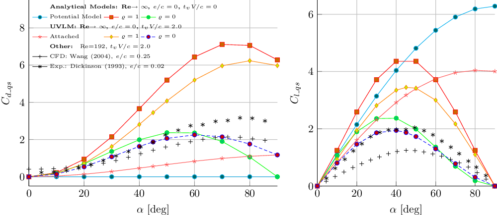
Wang et al(Reference Wang, Birch and Dickinson24) normalise their measured unsteady loads by the maxima of the corresponding translational quasi-steady forces and claimed that this method normalises away the section geometry and thickness. In this current effort it is hypothesised that the method also normalises away the effect of the Reynolds number. To compare the current models with the experimental data the quasi-steady translation forces predicted by each model are needed.
The different curves of quasi-steady drag  $C_{d\_qs}$
and lift
 $C_{l\_qs}$
versus the angle-of-attack
 $\alpha$
obtained with the different models are presented in Fig. 2. The experimental results of Wang et al(Reference Wang, Birch and Dickinson24) and Dickinson and Götz(Reference Dickinson and Götz5) are also included in the plots for reference only since a comparison at this stage is not strictly valid due to the different Reynolds numbers and geometries. Dickinson and Götz(Reference Dickinson and Götz5) showed that the maximum lift and drag coefficients for early times (
 $t_vV/c=2$
) of an impulsively started wing increases with the Reynolds number. Their experiments were conducted at
 $\text{Re}=192$
whereas the theory corresponds to a flat plate with Re
 $\to\infty$
. Wang(Reference Wang36) (Section 3.2.2.) showed that a two-fold decrease in the thickness could produce approximately a 40% increase in the lift. Wang’s ellipse has a thickness ratio
 $e/c=0.25$
whereas for Dickinson’s flat plate
 $e/c=0.02$
. Therefore the larger Reynolds number and the zero thickness are responsible for the generally larger quasi-steady loads predicted by the present models as observed in Fig. 2.
Summary of quasi-steady drag and lift coefficients  $C_d$
and
 $C_l$
as a function of the angle-of-attack obtained with the different methodologies presented.

3.1.1 Potential flow model
For this model, the quasi steady translation lift and drag coefficients of a flat plate at a fixed angle-of-attack  $\alpha$
are well known theoretical results and are obtained from Equation (13) by setting
 $\omega=0$
and the time derivative terms to zero
 \begin{align} C_{l\_qs} = 2\pi \sin \alpha, && C_{d\_qs} =0. \end{align}
3.1.2 Modified force potential model
The quasi steady translation lift and drag coefficients of a flat plate at a fixed angle-of-attack  ${-\pi/2\le\alpha\le\pi/2}$
are obtained from Equation (20):
 \begin{align}\equationnumber{\normalfont(34)}C_{l\_{qs}} {}={}& \pi\sqrt{1+\varrho^2} \sin 2\alpha \cos \left(\alpha+\alpha_\varrho \right),\\[-6pt]\nonumber \end{align}
 \begin{align}\equationnumber{\normalfont(35)}C_{d\_{qs}} {}={}&2 \pi \sqrt{1+\varrho^2} \sin^2\alpha\sin \left(\alpha+\alpha_\varrho \right),\\[12pt]\nonumber\end{align}
with  $\tan\alpha_\varrho =1/{\varrho}$
.
Equations (34) and (35) show the  $\sin 2\alpha$
and
 $\sin^2 \alpha$
dependance of Rayleigh’s (Section 12.26 of ref. (Reference Milne-Thompson31)). It is observed that for
 $\varrho=0$
(
 $\alpha_\varrho=90^\circ$
), the model predicts zero drag at
 $\alpha=90^\circ$
, something which is clearly incorrect. However, the values at intermediate angles of attack up to 45
 $^\circ$
(which will most likely be the ones used for the normalisation of the loads) may still be adequate.
3.1.3 UVLM model
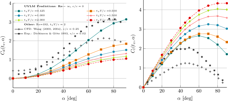
For the UVLM-based models, the quasi-steady forces are computed in a similar fashion as described by Wang et al(Reference Wang, Birch and Dickinson24) and Dickinson and Götz(Reference Dickinson and Götz5). A two-dimensional flat plate is “impulsively” set into constant velocity forward motion. The quasi steady lift and drag coefficients obtained at different nondimensional times  $t_vV/c$
with the different UVLM models are included in Appendix A. To be consistent with Wang et al(Reference Wang, Birch and Dickinson24), the quasi-steady loads are taken to be those obtained at a nondimensional time equal to
 $t_vV/c=2$
. The model labeled “UVLM attached” does not contain the force modification outlined previously and is used as a baseline for comparison.
3.2 Unsteady loads developed by flapping motions
The main results of this effort are presented in the following sections. In Sections 3.3 and 3.4, the unsteady forces generated by a flat wing section with two different set of kinematics are analysed and compared with the corresponding experimental data reported by Wang et al(Reference Wang, Birch and Dickinson24) and Dickinson et al(Reference Dickinson, Lehmann and Sane7), respectively. It is noted that in both of the experiments conducted by Wang et al and Dickinson et al a three-dimensional wing with the planform of a Drosophila wing undergoing prescribed three-dimensional flapping motions was used. The experimental apparatus used by those researchers (dynamically scaled robotic fly) is the same and the set-up similar. Therefore, the corresponding measured aerodynamic loads, which have been used in the present study, are three-dimensional in nature.
In view of the above, a discussion regarding the issues and validity of the comparison between two-dimensional models and three-dimensional experiments is required. This debate is elaborated in the discussion section.
3.3 Two-dimensional harmonic kinematics
These kinematics, given by Equations (36), were studied by Wang et al(Reference Wang, Birch and Dickinson24):
 \begin{align}X_O(t) =& \frac{A_f}{2}c\cos(\varpi t),\ \ \ \ \ Y_O(t) = 0\nonumber\\[5pt]
\varsigma(t) =& -\frac{\pi}{2}+\frac{\Theta}{2}\sin(\varpi t+\psi)\end{align}
Here,  $\left(X_O(t),Y_O(t)\right)$
are the global coordinates of the pivot O of the section (in this case, the centroid C),
 $\varsigma(t)$
is the angular orientation of the section with respect to the positive X axis (positive according to the right-hand rule; see Fig. 1(b)),
 ${\varpi=2\pi f_f}$
is the angular frequency,
 $A_f$
is the amplitude of the translational motion, and
 $\Theta$
is the amplitude of the rotational motion. The phase angles
 $\psi$
studied are
 $-45^\circ$
,
 $0^\circ$
, and
 $45^\circ$
for delayed, in phase, or advanced rotation with respect to the translation, respectively.
As mentioned earlier, the experiments conducted and the loads reported by Wang et al are for a three-dimensional wing with three-dimensional flapping kinematics. However, Wang et al do not provide enough information regarding the three-dimensional kinematics; instead, the motion  $X_O(t0)$
in Equation (36) was provided with
 $A_f$
being the two-dimensional projection (the secant) of the curvilinear path of the center of rotation of the wing section located at the 70% of the wing span.
3.3.1 Results
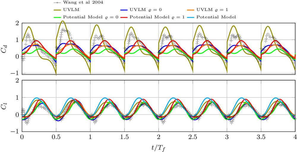
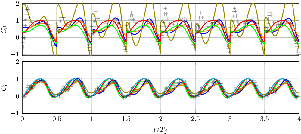
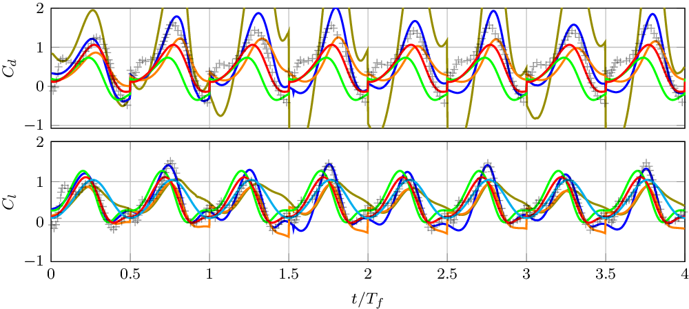
The comparison between experimental loads dataFootnote 2 and the models’ predictions is shown in Figs 2, 3 and 4. Qualitatively, it is observed that all the models are able to describe the shape and amplitude of the time history of the lift. With regard to the drag, the analytical model with  $\varrho=1$
and the UVLM with
 $\varrho=0$
stand out over the rest. However, neither of the models can capture the peaks that occur at the beginning of the stroke. A reason for that may be the presence of the end of stroke vortex at the stroke reversal that may be pushed down underneath the wing as the half-stroke begins and before the new leading edge vortex has grown completely. Also, it is obseved that the attached UVLM model predicts larger amplitudes of
 $C_d$
, especially for the symmetric and advanced rotation cases.
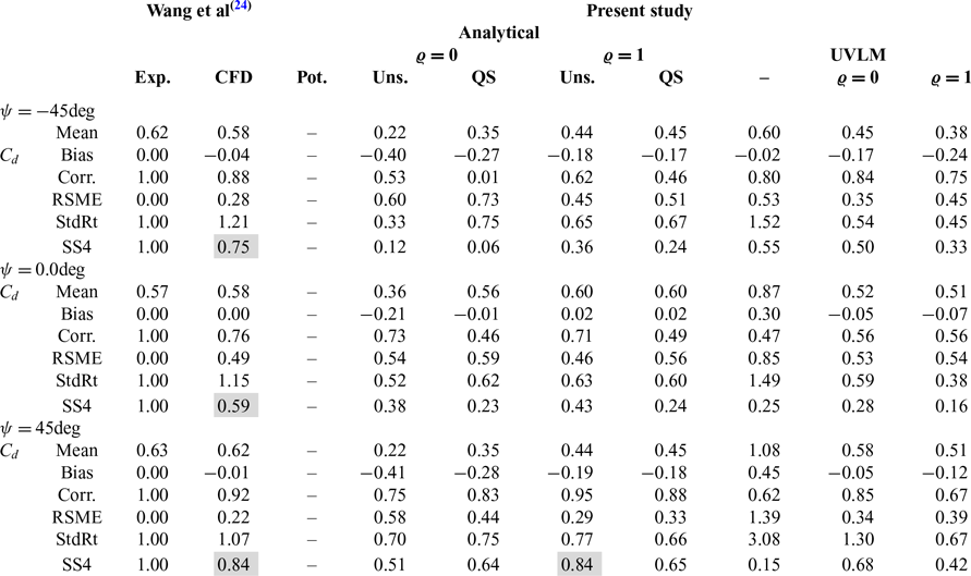
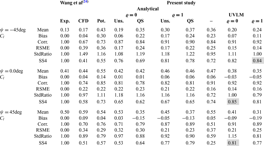
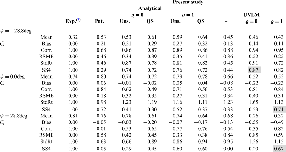
A quantitative error analysis is preformed and summarised in Tables 1 and 2. Also included in the table are the statistics of Wang’s CFD predictions. Furthermore, the statistics of the prediction of the translational quasi-steady (QS) version of each analytical model is also included. The ability of the model to reproduce the experimental data is summarised by the skill score (SS4), defined in Equation (37) (Equation (5) of ref. (Reference Taylor37) assuming that the maximum correlation attainable is  $R_0=1$
).
 \begin{equation}\text{SS4}=\frac{\left(1+R\right)^2}{4\left(\hat\sigma+1/\hat\sigma\right)^2}.\end{equation}
Here,  $\hat\sigma$
is the standard deviation ratio and R is the correlation coefficient. In Table 2, it is observed that the modified UVLM models achieve the highest value of SS4 in the prediction of
 $C_l$
for all of the values of
 $\psi$
analysed, even higher than the CFD model of Wang et al(Reference Wang, Birch and Dickinson24). Amongst the analytical models, the leading edge suction analogy (
 $\varrho=1$
) yields the best predictions of lift, with the unsteady model having a small advantage over the quasi-steady translation model. Regarding the
 $C_d$
the scores of the CFD simulations are the highest.
Comparison between  $C_d$
predictions, experiments and CFD(Reference Wang, Birch and Dickinson24) for different values of
 $\psi$
. Highlighted cells are the best SS4 values

Comparison between  $C_l$
predictions, experiments and CFD(Reference Wang, Birch and Dickinson24) for different values of
 $\psi$
. Highlighted cells are the best SS4 values

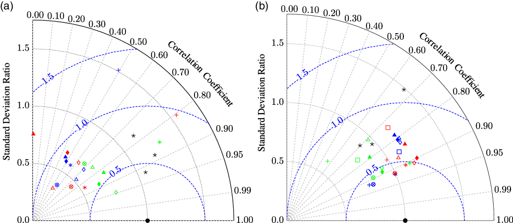
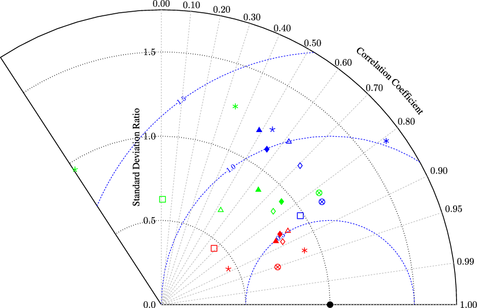
The error analysis is summarised graphically in Figs 6(a) and (b). It is observed in the diagram of Fig. 6(b) that the UVLM lift predictions are closer to the experiments. In the case of the drag, Fig. 6(a), the CFD predictions are closer to the experiments and the predictions of the models scattered around.
Normalised drag and lift for a delayed rotation flapping kinematic  $\phi\,\text{=}$
–45.0deg.

Normalised drag and lift for a symmetric rotation flapping kinematic  $\phi\,\text{=}$
0.0deg. Line references from Fig. 3.

Normalised drag and lift for a advanced rotation flapping kinematic  $\phi\,\text{=}\,\text{45.0}\text{deg}$
. Line references from Fig. 3.

Taylor diagrams summarising the error analysis of the models and CFD in the prediction of the aerodynamic load coefficients. Red:  $\psi\,\text{=}$
–45deg, blue:
 $\psi\,\text{=}$
0deg, green:
 $\psi\, \text{=} $
45deg.
 $\star$
: CFD(Reference Wang, Birch and Dickinson24),
 $+$
:UVLM,
 $*$
: UVLM
 $\varrho\,\text{=}\,0$
,
 $\otimes$
: UVLM
 $\varrho\,\text{=}\,1$
,
 $\square$
: Potential,
 $\triangle$
: Model
 $\varrho\,\text{=}\,0$
,
 $\lozenge$
: Model
 $\varrho \,\text{=}\, 1$
. Filled markers: Quasi-Steady. (a)
 $C_d$
. (b)
 $C_l$
.

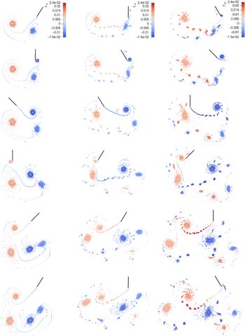
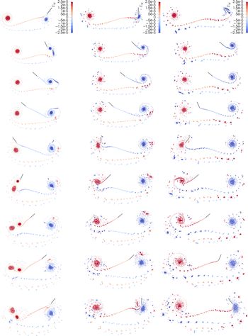
To complete the study, the wake evolutions for each case are shown in Fig. 7. It is observed that the wakes become less compact as the phase angle  $\psi$
increases from
 $-45$
to 45deg. This may be an indication of a more pronounced interaction between the wing and its wake for the symmetric and advanced rotation cases, as can be appreciated at the non-dimensional time 1.375. Also, this could explain why in general de model predictions are better for the delayed rotation case. Except for the absence of a leading edge wake and the persistence of the wake vorticity (due to the absence of viscous diffusion in the wakes), the wakes for the case
 $\psi=0$
bare similarity with the vorticity plots shown in Fig. 6 of ref. (Reference Wang, Birch and Dickinson24).
Wakes generated by a flat plate with kinematics (36) with delayed (left), symmetric (center) and advanced (right) rotation motion. From top to bottom, the instants of nondimensional time  $f_f t$
shown are approximately: 1.00, 1.125, 1.375, 1.625, 1.875 and 2.00.

3.4 Three-dimensional flapping kinematics
The robofly kinematics ( $\dot\phi$
,
 $\dot\varsigma$
, Fig. 8) given by (38)Footnote 3 were employed by Dickinson et al(Reference Dickinson, Lehmann and Sane7).
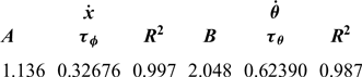
 \begin{align}\dot{X}(r,t)&=r\dot{\phi}(t)=-r\frac{\Phi \varpi}{\pi} A\text{erf}\left[\frac{\sin\varpi t}{\tau_\phi}\right]\\\dot{\varsigma}(t)&=-\frac{\Theta\varpi }{2\tau_\theta \sqrt{\pi}}B e^{-\frac{\sin^2( \varpi t+\psi)}{\tau_\theta^2}}\cos( \varpi t+\psi),\end{align}
where  $\text{erf}[\cdot]$
is the error function,
 ${\varpi=2\pi f_f}$
is the angular frequency, r is the spanwise distance from the hinge point,
 $\phi(t)$
is the stroke angle,
 $\Phi\triangleq [\text{rad}]$
is the stroke amplitude,
 $\Theta\triangleq [\text{rad}]$
is the incidence angle amplitude around
 $\varsigma=90^\circ$
. A, B,
 $\tau_\phi$
and
 $\tau_\theta$
are coefficients obtained through curve-fitting and reported in Table 3. In the cases studied
 $f_f=0.145$
Hz,
 ${\Phi=160}$
deg,
 $\Theta=100$
deg (corresponding to a mid-stroke angle-of-attack
 $\alpha=40$
deg) and
 $\psi =-28.8^\circ$
,
 $0.0^\circ$
,
 $28.8^\circ$
for delayed, symmetric and advanced rotation, respectively.
Values of the Coefficients in Equation (38)

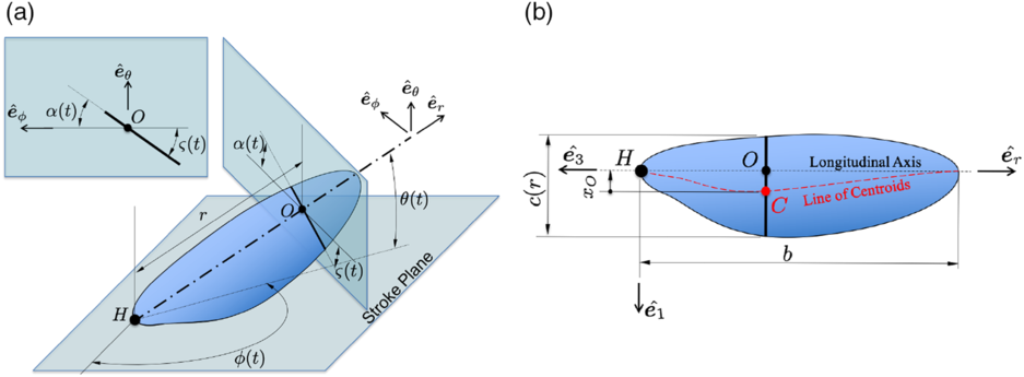
Flapping wing with a two-dimensional wing section at distance r highlighted. (a) Three-dimensional flapping wing. (b) Schematic planform of a wing.

The robobly wing parameters are only partially available in ref. (Reference Dickinson, Lehmann and Sane7)Footnote 4; thus, it not possible to use the blade-element extension of models. Therefore, the comparison has to be done with caution as it may not be strictly valid to compare three-dimensional results with two-dimensional predictions. A characteristic wing section with  $c=S/b=0.0668$
m (wing mean chord) and located at
 $r/c=\sqrt{r_{11}^{2}}/c=0.484$
(wing radius of gyration) is selected for the study. This section travels an arclength of
 $6.61c$
during each half stroke.
3.4.1 Results
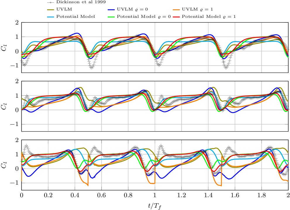
The comparison of the normalised  $C_l$
data (drag data not available) from the experiments and the predictions of the models is presented in Fig. 9. It is observed that models qualitatively describe the phase and amplitude of the time signals. However, as in the previous case, the peaks at the beginning of the stroke are not well captured by any of the models. Also, the potential and attached UVLM models shown an increasing phase shift with the data in going from the delayed to the advanced rotation. The statistical indicators of the predictions are summarised in Table 4 and in a Taylor diagram in Fig. 11. From this analysis, it is concluded that in general, the UVLM model with leading edge suction analogy (
 $\varrho=1$
) is the best to estimate of the lift forces developed by the robofly. However, it is observed that the quality of the predictions worsen as the phase between the rotation and the translational motion goes from delayed to advanced.
Comparison between normalised lift predicted by the models and the experimental data.

Comparison between  $C_l$
predictions of the models and Dickinson et al (7) experiments. Highlighted cells are the best SS4 values

Wakes generated by a flat plate with kinematics (38) with delayed (left), symmetric (centre) and advanced (right) rotation. From top to bottom, the instants of nondimensional time  $f_f t$
shown are approximately: 1.000, 1.125, 1.250, 1.375, 1.500, 1.625, 1.750, 1.875 and 2.000.

Taylor diagram summarising the error analysis of normalised  $C_l$
predictions of the models. Refer to Fig. 6(a) for color and mark references.

Finally, the wakes developed by the wing section are shown in Fig. 10. As in the previous case, it is observed that the wakes become more disturbed in going from the delayed to the advanced rotation kinematics. The wakes reveal the vortex structures consisting of two large counter rotating starting vortices which are generated at the beginning of each half-stroke. As in the previous case, the more evident wake interaction for the symmetric and advanced rotation cases could be a reason to explain why the model predictions worsen for these cases.
4.0 DISCUSSION
In the first study (Section 3.3), a harmonic-type kinematics was examined and the results of the models were compared with experimental and CFD data. Judging by the SS4 metric it was found that the UVLM model was quite superior to the CFD model regarding the prediction of the lift. The correlation of the  $C_l$
predictions ranges from 0.89 to 0.92, whereas for the CFD simulations it ranges from 0.67 to 0.92. Thus, with the UVLM model, one has the ability to describe the time history of the lift. The UVLM predictions of drag, on the other hand, were not as good as those of the CFD model, but still show a correlation with the experimental data that can be considered good enough depending the purpose. The correlation of the CFD model for the
 $C_d$
ranges from 0.76 to 0.92, whereas for the UVLM model, the correlation ranges from 0.56 to 0.85. The lowest values correspond to the kinematics with symmetric rotation for both the UVLM and the CFD. The correlations of these two models with the experiments are not as different as one may have expected based on the huge complexity gap between them. Therefore, this comparison allows to put into perspective the real benefit of pursuing high-fidelity, high-computational cost CFD models in this situation when a good enough estimate is possible with a low-fidelity, low-computational cost UVLM model.
In the second study (Section 3.4), a three-dimensional motion of a wing was studied with the two-dimensional aerodynamic models. Judging by the SS4 metric, it was found that the modified UVLM model is superior to the analytical models when predicting the experimental lift. The modified UVLM model attains very high correlations that range from 0.81 to 0.94, again showing that the model is able to capture the time history pattern of the load. However, large biases were observed, indicating large under prediction of the mean values. Among other reasons, these differences may be due to the two-dimensional approximation of the three-dimensional phenomenon, to the assumptions made regarding the unknown geometry of the wing, and to the simplifications of the models. For this last case, the three-dimensional effects are suspected to be more important than in the first study due to the pronounced circular trajectory of the characteristic section considered (it travels an arclength of  $6.61c$
compared to
 $2.8c$
for the harmonic kinematics).
It was found that for the harmonic kinematics, the predictions of the UVLM model with  $\varrho=0$
were best for the symmetric and advanced rotation cases. For the delayed rotation, the UVLM with
 $\varrho=1$
was found to be best. This may be an indication of the average importance of the leading edge vortex throughout each half-stroke and the importance of the kinematics. Also, it highlights a drawback of the approach in that
 $\varrho$
is chosen and fixed throughout the motion. It is expected that the contribution of the leading edge vortex is initially small at the stroke reversal (
 $\varrho\to 0$
), attains its maximum value once it has grown fully (
 $\varrho\to1$
), and even reverses its direction at stroke reversals if the vortex is pushed underneath the wing (
 $\varrho \to -1$
). For the harmonic kinematics, the delayed rotation seems to favor the delayed stall mechanism compared to the symmetric and advanced rotation cases. This may be due to the lesser interaction of the wing with the disturbing trailing edge wake.
For the three-dimensional kinematics, the opposite was observed; that is to say, the UVLM with  $\varrho=0$
produced the best estimates of lift for the delayed rotation case, and
 $\varrho=1$
for the symmetric and advanced rotation cases. Again, this highlights the importance of the kinematics in the delayed stall mechanism. It is noted that this kind of kinematics is characterised by portions of almost constant speed and angle-of-attack. Those conditions are expected to contribute positively to the stationarity of the leading edge vortex. This could be the reason why the leading edge suction analogy does a better job at predicting the loads for this kinematics compared to the harmonic kinematics, characterised by constantly varying speed and angle-of-attack.
The above-mentioned observations point out the importance of the kinematics on the loads generated by flapping wing as a particular set may help exploit the delayed stall mechanism and others not. An improvement of the approach presented here would be to introduce a dependence of  $\varrho$
on the kinematics or on the flow conditions at the leading edge. This conclusion is consistent with the results of Chen et al(Reference Chen, Colonius and Taira39), who found that the nondimensional leading edge vortex formation time (hence the lift augmentation time scale) is a function of the Reynolds number, the angle-of-attack, and the acceleration. Also, the UVLM models could be improved if a suitable description of the leading edge separation is included. Finally, it is observed that the introduction of a wake model (UVLM model) has produced a slight enhancement in the predictions with respect to the analytical models.
4.1 On the comparison of results from two-dimensional models and three-dimensional experiments
Not necessarily in order of importance, the following aspects arise with regard to the validity of a comparison between the results of two-dimensional models and three-dimensional experiments. First, even for a uniform incoming flow, the formation and persistence of the wing tip vortex produces a non uniform distribution of the load along the span (because of the downwash effect). The influence of this tip vortex over the wing weakens with the distance from the tip. Therefore, a two-dimensional representation of the wing should correspond to a characteristic section that is “sufficiently” far from the tip.
Second, the rotational motion of the wing about its root would in principle induce an spanwise flow due to centrifugal acceleration. As mentioned in the introduction, the task of stabilizing the leading edge vortex was attributed to this axial flow; however, as pointed out by Wang et al(Reference Wang, Birch and Dickinson24) in their discussion, several flow visualisations have shown no evidence of such a flow. Moreover, Wang et al argue that a spanwise flow is not needed to stabilise the leading edge vortex as long as the flapping stroke amplitude does not exceed 4 chords (something that is approximately true in most flying beings). This travel limit is intimately related to the time scale of the vortex formation for a translating two-dimensional wing section. This point of view is also supported by the study of Chen et al(Reference Chen, Colonius and Taira39) who propose a “universal” scale of four to five chords for two-dimensional delayed stall lift augmentation. With these ideas in mind, one could argue that a suitable two-dimensional model could potentially reproduce the delayed stall mechanism of a three-dimensional flapping wing.
The last issue to be discussed arises also from the beating motion about the root of the wing (speed varies with the distance to the root), the rotation  $\omega$
of the wing about its longitudinal axis, and the nonuniform chord distribution of the wing. Analysing Equation (20), it is noted that the different terms in the two-dimensional force scale differently with respect to the chord c and r of the wing section considered. Therefore, different, non-proportional force histories are obtained at different values of r. For example, if the blade-element theory is used to estimate the three-dimensional force on the wing, the three-dimensional normal force coefficient would be estimated by:
 \begin{align}C_n=\frac{{\textbf{\textit{F}}}_{\text{3D}}\cdot \hat{\textbf{\textit{n}}}}{\frac{1}{2}\rho V_{\text{ref}}^2\mathcal{S}}\approx\frac{1}{\frac{1}{2}\rho V_{\text{ref}}^2\mathcal{S}}\hat{\textbf{\textit{n}}}\cdot\int_0^b {\textbf{\textit{F}}}_{\text{2D}}(r,\theta,\phi) dr,\end{align}
where b is the wing span and  $\mathcal{S}$
is the wing planform area. For a flapping wing as the one schematically shown in Figure 8, the velocity of a point O along the longitudinal axis, at a distance r from the root point H, can be expressed in a stroke plane-based spherical coordinate system as
 ${{\textbf{\textit{v}}}_O(r) =r\dot{\phi} \cos\theta\hat{\textbf{\textit{e}}}_\phi+r\dot\theta\hat{\textbf{\textit{e}}}_\theta}$
, where
 $\dot{\phi}$
is the stroke angular speed and
 $\dot{\theta}$
the elevation angular speed. The speed of point O is given by
 $V_O=r\sqrt{\dot{\phi}^2\cos^2\theta+\dot{\theta}^2}$
.
Upon applying the blade-element theory (39) to a rigid flat wing (with  ${\textbf{\textit{F}}}_{\text{2D}}(r,\theta,\phi)$
given by Equation (13) or (20)), and considering
 $U_\infty=0$
and
 $\dot\theta=0$
for simplicity, the two-dimensional term purely related to the translational motion leads to the following integral
 \begin{align}\int_0^b c(r)V_O^2(r)dr&=\dot\phi^2\int_0^b c(r) r^2 dr=\dot\phi^2\int_\mathcal{S} r^2 d\mathcal{S}=\dot\phi^2 r_{11}^2 \mathcal{S}=\dot\phi^2 r_{11}^2 \bar{c}b,\end{align}
where  $r_{11}$
is the radius of gyration with respect to the
 $\hat{{\textbf{\textit{e}}}_1}$
direction. From Equation (40), it is observed that one could choose a characteristic section with chord equal to the wing’s mean geometric chord (
 $\bar{c}=\mathcal{S}/b$
) and translational speed given by
 $V_{\text{ref}}=r_{11}\dot{\phi}$
. This choice, which is the one adopted in the study of Section 3.4, is such that the two-dimensional force per unit span correctly describes the translation term of the three-dimensional aerodynamic force per unit span (since the two-dimensional model will predict a translational force proportional to
 ${\bar{c}V_{\text{ref}}^2= \dot{\phi}^2r_{11}^2\mathcal{S}/b}$
). However, this choice may not lead to the correct weighing of the remaining terms. For example, for the rotational term the blade-element theory leads to
 \begin{align}\int_0^b \omega c^2(r)V_O(r) dr&= \omega\dot\phi \int_0^b c^2 r dr= \omega\dot\phi \int_\mathcal{S} c r d\mathcal{S} \ne\omega \bar{c}^2V_{\text{ref}} b=\omega\dot\phi \bar{c} r_{11}\mathcal{S}.\end{align}
Therefore, this rotational component of the force is not correctly accounted for by a two-dimensional model when  $\bar{c}$
and
 $V_{\text{ref}}=r_{11}\dot{\phi}$
are chosen. Even when
 $\omega=0$
, still the two-dimensional translational added mass term remains and leads to
 \begin{align}\int_0^b \frac{\pi\rho}{4}c^2(r) \frac{dV_O(r)}{dt} dr&=\ddot\phi\int_\mathcal{S} \frac{\pi\rho}{4}c r d\mathcal{S}\ne\frac{\pi\rho \bar{c}^2}{4}\frac{dV_{\text{ref}}}{dt}b = \ddot\phi \frac{\pi\rho}{4}\bar{c} r_{11}\mathcal{S},\end{align}
so the conclusion is the same as before. The last integral term is called the first moment of the virtual mass ( $v_1$
) by Ellington(Reference Ellington40).
The above discussion leads to the conclusion that the choice made in this work of  $r=r_{11}$
 $c=\bar{c}$
, makes the two-dimensional force models consistent with the three-dimensional force only with regard to the translation. A more appropriate approach would be, as indicated previously, to extend the two-dimensional model to three dimensions by using a suitable theory. Also, through this discussion, the authors emphasize the difficulties and the importance of complete information regarding the wing shape and area moments to replicate the experimental data in the literature. Even with those difficulties, the two-dimensional force models presented are still able to capture the main features of the three-dimensional lift histories. For the kinematics analysed in Section 3.4, the translational added mass terms as well as the large rotational speeds
 $\omega$
, are confined at the end-of-stroke (approximately constant translation and rotation speed throughout the half-stroke). This may help explain why the two-dimensional models can still describe the three-dimensional loads for that case.
5.0 CONCLUSIONS
In this effort, a first of its kind comparison was carried out amongst several two-dimensional aerodynamic models in their ability to predict the loads developed by a flapping wing. This study has relevance in the field of bioinspired flapping wings micro-air-vehicles because it provides a basis for their aerodynamic design. Theoretical or analytical models are a suitable option to obtain quick estimates and characterisation and to obtain trends. Computational models are suitable for the detailed description of the flow physics once the design has been fixed and to obtain more accurate estimations of the loads, with the caveat of requiring extensive computational resources. This work shows that depending on the specific purpose, an analytical model can be good enough to predict the lift and drag on a flapping wing without the need of a detailed description of the flow field. However, it is pointed out that the kinematics are utterly important to determine the relative importance of the delayed stall mechanism and the selection of the adequate model accordingly. Besides the error analysis, the novelty of this effort lies in the modification of the loads computed through both the potential and UVLM models with a generalisation of the leading edge suction analogy.
It was observed that both the analytical and UVLM approaches with modified loads are able to reproduce the main characteristics of the time history of lift and drag for the harmonic kinematic case. For this case, the lift predictions are comparable and sometimes better than the predictions of a CFD model reported by other researchers. The predictions of drag, on the other hand, show that the method proposed still needs improvements. Finally, the results presented support the statement that normalising the loads by the equivalent quasi-steady translational force eliminates the dependance of the loads on the Reynolds number and that the physics of low Reynolds number flapping can be estimated with inviscid theories.
APPENDIX
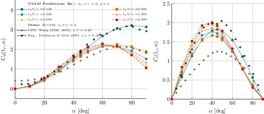
Drag (left) and Lift (right) coefficients as a function of the angle-of-attack obtained with the (unmodified) UVLM model at different nondimensional times  $t_{v} V/c$
.

Drag (left) and Lift (right) coefficients as a function of the angle-of-attack obtained with the UVLM model with  $\varrho\,\text{=} \,\text{0}$
at different nondimensional times
 $t_{v} V/c$
.

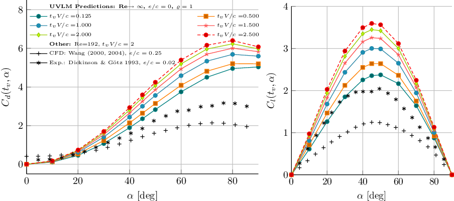
Drag (left) and Lift (right) coefficients as a function of the angle-of-attack obtained with the UVLM model with  $\varrho\,\text{=}\,\text{1}$
at different nondimensional times
 $t_{v} V/c$
.

A.0 QUASI-STEADY TRANSLATIONAL FORCE COEFFICIENTS COMPUTED WITH THE UVLM
A two-dimensional flat plate is “impulsively” set into constant velocity forward motion. The lift and drag coefficients obtained at different nondimensional times  $t_vV/c$
are shown in Figs A.1, A.2, and A.3 for the baseline UVLM (unmodified) and for values of
 $\varrho=0$
and 1. It is pointed out that despite the differences in the maximum values, the shape of the curves of
 $C_l$
and
 $C_d$
are similar to that of the experiments. To be consistent with Wang et al(Reference Wang, Birch and Dickinson24), the quasi-steady loads are taken to be those obtained at a nondimensional time equal to
 $t_vV/c=2$
. These are the curves that where finally plotted in Fig. 2.