1 Introduction
It is well known that solid particles suspended in a turbulent flow may exhibit a non-trivial spatial distribution as a consequence of their hydrodynamic interaction with coherent flow structures (Eaton & Fessler Reference Eaton and Fessler1994). The resulting spatial structure of the dispersed phase, in turn, is key to understanding many technologically relevant aspects of these systems, such as particle collision statistics, dispersion/mixing behaviour as well as the particles’ impact upon the carrier phase. It is therefore not a surprise that much effort has been devoted in the past to the understanding of the mechanisms responsible for the formation of agglomerations of particles in turbulent flows. In the following review we will for the sake of brevity focus our attention on the idealized flow configuration of (approximately) homogeneous-isotropic turbulence.
Let us first consider the case of small inertial particles (i.e. of sub-Kolmogorov size). The formation of clusters has indeed been observed in many laboratory experiments in the presence of gravity (e.g. Aliseda et al.
Reference Aliseda, Cartellier, Hainaux and Lasheras2002; Wood, Hwang & Eaton Reference Wood, Hwang and Eaton2005), and under conditions of micro-gravity (Fallon & Rogers Reference Fallon and Rogers2002). It has also been often reproduced in direct numerical simulations with point particles under the assumption of Stokes drag (e.g. Squires & Eaton Reference Squires and Eaton1991; Bec et al.
Reference Bec, Biferale, Boffetta, Celani, Cencini, Lanotte, Musacchio and Toschi2006; Calzavarini et al.
Reference Calzavarini, Kerscher, Lohse and Toschi2008). A number of studies suggest that clustering of sub-Kolmogorov particles is most intense when the Stokes number
 $St$
(defined as the ratio between the relevant particle and fluid time scales) takes values of order unity with respect to the dissipative scales of the turbulent carrier flow (Hogan & Cuzzi Reference Hogan and Cuzzi2001; Balachandar & Eaton Reference Balachandar and Eaton2010; Monchaux, Bourgoin & Cartellier Reference Monchaux, Bourgoin and Cartellier2012). This conclusion, however, somewhat depends upon the measure which is chosen for quantifying the intensity of clustering, and Yoshimoto & Goto (Reference Yoshimoto and Goto2007) have observed in their point-particle simulations that clustering occurs over a substantial range of values of the Stokes number, with different flow scales contributing accordingly. In a recent experimental study on polydisperse particles in grid-generated wind-tunnel turbulence, Sumbekova et al. (Reference Sumbekova, Cartellier, Aliseda and Bourgoin2016) conclude that the intensity of particle clustering (quantified by means of Voronoï tessellation analysis) is practically insensitive to the particles’ dissipation-scale Stokes number.
When investigating the statistical relation between particle positions and the local topology of the flow field, it is often found that sub-Kolmogorov particles are preferentially located in low-vorticity, strain-dominated regions (e.g. Squires & Eaton Reference Squires and Eaton1991; Sundaram & Collins Reference Sundaram and Collins1997; Bec et al.
Reference Bec, Biferale, Boffetta, Celani, Cencini, Lanotte, Musacchio and Toschi2006; Balachandar & Eaton Reference Balachandar and Eaton2010). The mechanism for this type of preferential particle accumulation has traditionally been linked to the action of coherent vortices. Based on an asymptotic expansion argument, Maxey (Reference Maxey1987) has proposed that small particles should centrifuge out of vortices due to their inertia, i.e. that particle clustering should indeed occur in low-vorticity regions. The aforementioned evidence can then be taken as an indication of the effectiveness of the centrifugal effect. However, since the analysis of Maxey (Reference Maxey1987) strictly only applies to the simplest point-particle model in the limit of small Stokes numbers, it is questionable how preferential accumulation could be caused by this mechanism at larger values of
 $St$
.
Various authors have investigated the structure of the disperse phase from the Lagrangian point of view. Starting from a description of the relative motion of a pair of particles, both Zaichik & Alipchenkov (Reference Zaichik and Alipchenkov2003) and Chun et al. (Reference Chun, Koch, Rani, Ahluwalia and Collins2005) have constructed models which are able to predict the radial-distribution function (RDF) based upon prior knowledge about statistical features of the carrier flow. The former approach has since been refined (Zaichik & Alipchenkov Reference Zaichik and Alipchenkov2007), and it is a priori applicable to the entire range of Stokes numbers. Note that the clustering mechanism inherent in the description of Zaichik & Alipchenkov (Reference Zaichik and Alipchenkov2007) is non-local due to the fact that the relative motion of two particles is a function of the history of the fluid velocity gradient tensor along the particle paths (cf. also the recent review by Gustavsson & Mehlig Reference Gustavsson and Mehlig2016). Bragg & Collins (Reference Bragg and Collins2014) have shown that for Stokes numbers
 $St\geqslant O(1)$
this non-local-in-time effect starts to outweigh the local centrifugal mechanism. Bragg, Ireland & Collins (Reference Bragg, Ireland and Collins2015b
) further argue that the non-local clustering mechanism is additionally biased by preferential sampling of strain-dominated regions along the particle paths, leading to the observed statistical correlation between particle locations and such fluid regions even in the Stokes number regime where the centrifugal mechanism alone is not expected to be efficient.
Another point of view on clustering of point particles in homogeneous-isotropic turbulence has been proposed by Chen, Goto & Vassilicos (Reference Chen, Goto and Vassilicos2006) and Goto & Vassilicos (Reference Goto and Vassilicos2006) in two dimensions, and later by Goto & Vassilicos (Reference Goto and Vassilicos2008) and Coleman & Vassilicos (Reference Coleman and Vassilicos2009) in the three-dimensional setting. These authors have established a link between the accumulation of point particles and the local properties of the fluid acceleration field, which is based upon the observation by Maxey (Reference Maxey1987) that in the limit of small particle inertia (i.e. small Stokes number) the particle velocity deviates from the local fluid velocity proportionally to the fluid acceleration. This effect has been termed ‘sweep-stick’ mechanism, since it relates to the sweeping of particles by the fluid flow field and their ‘sticking’ at zero-acceleration points. A recent paper by Bragg, Ireland & Collins (Reference Bragg, Ireland and Collins2015a
) has challenged the effectiveness of the sweep-stick mechanism at length scales
 $r$
when the scale-dependent Stokes number is of the order of (or exceeds) unity,
 $St_{r}\geqslant O(1)$
. These authors argue that, while for
 $St_{r}\ll 1$
it is the preferential sampling of low-vorticity regions of the fluid velocity field ‘coarse grained’ at the length
 $r$
which dominates, for
 $St_{r}\geqslant O(1)$
the essential mechanism is rather a combination of the preferential sampling and of the above-mentioned non-local effect.
Much less is known about the dynamics of particles with diameters equal to or larger than the Kolmogorov scale. Systematic studies of finite-size effects have been carried out in von Kármán flows (which feature a central region of approximately homogeneous-isotropic turbulence) by Voth et al. (Reference Voth, la Porta, Crawford, Alexander and Bodenschatz2002), Brown, Warhaft & Voth (Reference Brown, Warhaft and Voth2009) and Volk et al. (Reference Volk, Calzavarini, Lévêque and Pinton2011), while Qureshi et al. (Reference Qureshi, Bourgoin, Baudet, Cartellier and Gagne2007) have performed a complementary analysis in grid turbulence in a wind tunnel. In all these studies the particles were approximately neutrally buoyant, and the concentration was sufficiently low such that collective effects can be excluded. It was found that the normalized probability density function (p.d.f.) of particle acceleration roughly collapses on a functional form which is consistent with the log-normal scaling of the acceleration vector magnitude first suggested by Mordant, Crawford & Bodenschatz (Reference Mordant, Crawford and Bodenschatz2004) for fluid particles. Finite-size effects can then conveniently be described by the acceleration variance alone, which is found to be reasonably well represented by Kolmogorov inertial-range scaling, supposing that the scales which determine the particle acceleration are of the same order as the particle diameter
 $D$
itself, i.e. implying a
 $D^{-2/3}$
power law. Note that Qureshi et al. (Reference Qureshi, Arrieta, Baudet, Cartellier, Gagne and Bourgoin2008) have extended the analysis to heavy particles with densities up to 66 times the fluid density, suggesting a non-trivial influence of the density ratio upon the particle acceleration variance. The more recent measurements of Fiabane et al. (Reference Fiabane, Zimmermann, Volk, Pinton and Bourgoin2012) are to our knowledge the only available source of experimental data on clustering of finite-size particles suspended in sustained, approximately homogeneous-isotropic turbulence. They investigated two particle types (either neutrally buoyant or with a density of 2.5 times that of the fluid) in a chamber with random large-scale turbulence forcing. The authors observe that in the same range of the Stokes number (approximately from 0.25 to 1.25) the density-matched particles do not form clusters, while the heavy particles clearly do. This result demonstrates that the Stokes number alone is not a sufficient parameter for determining the spatial distribution of finite-size particles. Unfortunately it is not possible to rigorously separate the effect of gravity from the effect of enhanced particle inertia in the laboratory measurements of Qureshi et al. (Reference Qureshi, Arrieta, Baudet, Cartellier, Gagne and Bourgoin2008) and Fiabane et al. (Reference Fiabane, Zimmermann, Volk, Pinton and Bourgoin2012), which is where numerical simulations can contribute to fill the knowledge gaps.
Turning to numerical work, the first simulations of finite-size particles suspended in forced, homogeneous-isotropic turbulence were performed by Ten Cate et al. (Reference Ten Cate, Derksen, Portella and Van Den Akker2004) in moderately dense systems where the solid/fluid density ratio was above unity and gravity set to zero. Yeo et al. (Reference Yeo, Dong, Climent and Maxey2010) have considered similar systems (using the force-coupling approach of Lomholt & Maxey Reference Lomholt and Maxey2003), while varying the density ratio over a certain range. On the other hand, Homann & Bec (Reference Homann and Bec2010) have carried out a systematic study of finite-size effects upon the motion of a single, neutrally buoyant particle in forced, homogeneous-isotropic turbulence. The parameter space was later extended by Cisse, Homann & Bec (Reference Cisse, Homann and Bec2013) and Cisse (Reference Cisse2015) to larger turbulent Reynolds numbers and particle sizes. Together, these numerical studies provide important information on the scaling of a number of particle-related properties (cf. discussion in § 3.1). However, the aspect of preferential particle location with respect to coherent structures has not been addressed by these authors.
In the present contribution we have performed DNS (direct numerical simulation) describing the motion of a dilute suspension of particles with diameter larger than the Kolmogorov length (up to 11 times), while fully resolving the flow around each particle. We consider inertial particles with a mass density of 1.5 times the fluid density. This parameter point has been chosen in order to be able to address the effects of gravity and turbulence upon the motion of a finite-size particle collective separately: the former effect has been singled out in the study of Uhlmann & Doychev (Reference Uhlmann and Doychev2014) while the latter is the subject of the present work. Ultimately we are interested in analysing the combined effects of gravity and turbulence upon the motion of heavy particles; this next step will be considered in a forthcoming contribution. In the present work a turbulent flow is maintained statistically stationary with the aid of large-scale random forcing. This allows us to obtain information about the fully developed state of the particulate phase in response to a well-defined turbulent carrier flow, which is difficult to achieve when decaying turbulence is considered (as done e.g. in the studies of Doychev & Uhlmann Reference Doychev, Uhlmann, Balachandar and Sinclair Curtis2010; Lucci, Ferrante & Elghobashi Reference Lucci, Ferrante and Elghobashi2010, Reference Lucci, Ferrante and Elghobashi2011). The main objective of the present work is to contribute to the clarification of the tendency of finite-size particles to concentrate locally in a turbulent flow. Here we perform – for the first time to our knowledge – a detailed analysis of the particles’ preferential location with respect to coherent structures of the turbulent flow field.
This paper is organized as follows. The chosen methodology is described in terms of the numerical method as well as the flow configuration and parameter set in § 2. Section 3 is devoted to the presentation of the results, where we set out to quantify the feedback of the dispersed phase upon the carrier phase, and where we document the basic Eulerian and Lagrangian statistics in relation to previous results from the literature. Next we address more specifically the question of particle clustering by quantifying the deviation from a random arrangement. In the final part we then explore the relation between coherent vortices and particle locations, before turning to the analysis of the role of the fluid acceleration field in the present context. The paper closes with a summary and discussion in § 4.
2 Computational set-up
2.1 Numerical method
The basic numerical method employed in the present simulations has been described in detail by Uhlmann (Reference Uhlmann2005a
); it has recently been extended by including a random turbulence-forcing scheme (Chouippe & Uhlmann Reference Chouippe and Uhlmann2015). The incompressible Navier–Stokes equations are solved by a fractional step approach with an implicit treatment of the viscous terms (Crank–Nicolson) and a low-storage, three-step Runge–Kutta scheme for the nonlinear terms. The spatial discretization employs second-order central finite differences on a staggered mesh which is uniform and isotropic (i.e.
 $\unicode[STIX]{x0394}x=\unicode[STIX]{x0394}y=\unicode[STIX]{x0394}z=\text{cst}.$
). The no-slip condition at the surface of moving solid particles is imposed by means of a specifically designed immersed boundary technique (Uhlmann Reference Uhlmann2005a
). This gives rise to an additional volume force term in the momentum equation which we denote as
 $\boldsymbol{f}^{(ibm)}$
. In this setting the equations which describe the motion of an incompressible fluid with constant density
 $\unicode[STIX]{x1D70C}_{f}$
and constant kinematic viscosity
 $\unicode[STIX]{x1D708}$
can be written as follows:
 $$\begin{eqnarray}\displaystyle & \displaystyle \frac{\unicode[STIX]{x2202}\boldsymbol{u}_{f}}{\unicode[STIX]{x2202}t}+(\boldsymbol{u}_{f}\boldsymbol{\cdot }\unicode[STIX]{x1D735})\boldsymbol{u}_{f}+\frac{1}{\unicode[STIX]{x1D70C}_{f}}\unicode[STIX]{x1D735}p=\unicode[STIX]{x1D708}\unicode[STIX]{x1D6FB}^{2}\boldsymbol{u}_{f}+\boldsymbol{f}^{(t)}+\boldsymbol{f}^{(ibm)}, & \displaystyle\end{eqnarray}$$
 $$\begin{eqnarray}\displaystyle & \displaystyle \unicode[STIX]{x1D735}\boldsymbol{\cdot }\boldsymbol{u}_{f}=0, & \displaystyle\end{eqnarray}$$
 $\boldsymbol{u}_{f}$
denotes the fluid velocity vector,
 $p$
the hydrodynamic pressure and
 $\boldsymbol{f}^{(t)}$
is a volume force introduced in order to generate and maintain turbulent motion. Chouippe & Uhlmann (Reference Chouippe and Uhlmann2015) provide the details of the presently chosen temporal integration of the Navier–Stokes equations in the presence of solid particles and artificial turbulence forcing.
On the other hand, the motion of the particles is computed from the Newton equations for linear and angular motion of rigid bodies, driven by buoyancy, hydrodynamic force/torque and contact forces (in case of particle–particle collisions). Since the particle suspensions under consideration here are dilute, collisions occur infrequently. In fact it is found that the average collision-free period is of the order of one large-eddy time scale (or, equivalently, of the order of 50 Kolmogorov time scales) for the systems simulated herein. Therefore, in the present work, particle contact is treated by a simple repulsive force mechanism (Glowinski et al. Reference Glowinski, Pan, Hesla and Joseph1999) formulated such as to keep colliding particles from overlapping non-physically. In the case of dense particle arrangements, the discrete element method of Kidanemariam & Uhlmann (Reference Kidanemariam and Uhlmann2014) can be employed instead.
The computational code has been extensively validated in unbounded flows as well as in wall-bounded shear flows (Uhlmann Reference Uhlmann2005a ,Reference Uhlmann and Sommerfeld b , Reference Uhlmann, Wesseling, Oñate and Périaux2006, Reference Uhlmann2008; Uhlmann & Dušek Reference Uhlmann and Dušek2014; Kidanemariam & Uhlmann Reference Kidanemariam and Uhlmann2014; Chouippe & Uhlmann Reference Chouippe and Uhlmann2015).
2.2 Flow configuration and parameters
Before turning to the description of the flow configuration, let us first fix some notational details. The usual Reynolds decomposition of the fluid phase velocity is introduced, where the average
 $\langle \cdot \rangle _{\unicode[STIX]{x1D6FA}_{f}}$
is computed over the region
 $\unicode[STIX]{x1D6FA}_{f}$
filled with fluid, viz.
 $$\begin{eqnarray}\displaystyle \boldsymbol{u}_{f}(\boldsymbol{x},t)=\langle \boldsymbol{u}_{f}\rangle _{\unicode[STIX]{x1D6FA}_{f}}(t)+\boldsymbol{u}_{f}^{\prime }(\boldsymbol{x},t). & & \displaystyle\end{eqnarray}$$
The corresponding kinetic energy of the fluctuations is then defined as
 $$\begin{eqnarray}\displaystyle k(t)={\textstyle \frac{1}{2}}\langle \boldsymbol{u}^{\prime }\boldsymbol{\cdot }\boldsymbol{u}^{\prime }\rangle _{\unicode[STIX]{x1D6FA}_{f}}={\textstyle \frac{3}{2}}u_{rms}^{2}(t), & & \displaystyle\end{eqnarray}$$
where the characteristic velocity scale
 $u_{rms}(t)$
has been defined simultaneously. We also define a dissipation rate averaged over the fluid phase, viz.
 $$\begin{eqnarray}\displaystyle \unicode[STIX]{x1D700}(t)=2\unicode[STIX]{x1D708}\langle S_{ij}^{\prime }S_{ij}^{\prime }\rangle _{\unicode[STIX]{x1D6FA}_{f}}, & & \displaystyle\end{eqnarray}$$
with
 $S_{ij}=(u_{i,j}+u_{j,i})/2$
. After further averaging
 $k(t)$
,
 $\unicode[STIX]{x1D700}(t)$
and
 $u_{rms}(t)$
over time in the statistically stationary interval (here indicated by simply omitting the argument ‘
 $t$
’), we can define the following global quantities: the Kolmogorov length scale
 $\unicode[STIX]{x1D702}=(\unicode[STIX]{x1D708}^{3}/\unicode[STIX]{x1D700})^{1/4}$
, the Taylor micro-scale
 $\unicode[STIX]{x1D706}=(15\unicode[STIX]{x1D708}u_{rms}^{2}/\unicode[STIX]{x1D700})^{1/2}$
and the associated Reynolds number
 $Re_{\unicode[STIX]{x1D706}}=\unicode[STIX]{x1D706}u_{rms}/\unicode[STIX]{x1D708}$
, the large-eddy length scale
 $L=k^{3/2}/\unicode[STIX]{x1D700}$
, the large-eddy turnover time
 $T=u_{rms}^{2}/\unicode[STIX]{x1D700}$
and the Kolmogorov time
 $\unicode[STIX]{x1D70F}_{\unicode[STIX]{x1D702}}=(\unicode[STIX]{x1D708}/\unicode[STIX]{x1D700})^{1/2}$
. The particle response time (based upon Stokes drag) is given by
 $\unicode[STIX]{x1D70F}_{p}=D^{2}\unicode[STIX]{x1D70C}_{p}/(18\unicode[STIX]{x1D708}\unicode[STIX]{x1D70C}_{f})$
; the Stokes number based upon Kolmogorov scales is then defined as
 $St_{\unicode[STIX]{x1D702}}=\unicode[STIX]{x1D70F}_{p}/\unicode[STIX]{x1D70F}_{\unicode[STIX]{x1D702}}$
, while a large-eddy Stokes number can be written as
 $St_{T}=\unicode[STIX]{x1D70F}_{p}/T$
. The particle velocity vector of the
 $i$
th particle is denoted by
 $\boldsymbol{u}_{p}^{(i)}(t)$
, and analogously for the position vector
 $\boldsymbol{x}_{p}^{(i)}(t)$
. The instantaneous average over the set of particles is denoted by the operator
 $\langle \cdot \rangle _{p}$
; as a shorthand we use the angular brackets without subscript ‘
 $\langle \cdot \rangle$
’ for the combined average over the respective phase and over time (in the statistically stationary interval).
In the present work we consider cubic boxes with side lengths
 ${\mathcal{L}}_{x}={\mathcal{L}}_{y}={\mathcal{L}}_{z}$
along the three Cartesian coordinate directions
 $(x,y,z)$
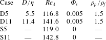
. The flow field and the particle motion are assumed triply periodic in space. Two different particulate flow cases are simulated, with global physical parameters as shown in table 1. The solid-to-fluid density ratio of
 $1.5$
as well as the global solid volume fraction of
 $0.005$
are kept the same in these two cases. The principal difference is the ratio of the particle diameter and the Kolmogorov scale, which measures
 $5.5$
and
 $11$
, respectively. Henceforth, these cases will be denoted as ‘D5’ and ‘D11’. Homogeneous-isotropic turbulence is generated and maintained with the aid of the random forcing scheme of Eswaran & Pope (Reference Eswaran and Pope1988), as described in detail by Chouippe & Uhlmann (Reference Chouippe and Uhlmann2015). Two slightly different turbulence-forcing parameter sets have been used for the two cases D5 and D11 (cf. table 2) which lead to mildly different Reynolds numbers of
 $Re_{\unicode[STIX]{x1D706}}=115$
and
 $142$
, respectively. In the following we will also use data from two single-phase simulations (denoted as ‘S5’ and ‘S11’) which have been performed with identical turbulence-forcing parameters as the respective particulate cases (note that the present case S11 is identical to case B of Chouippe & Uhlmann Reference Chouippe and Uhlmann2015).
The main physical parameters in the present simulations: length scale ratio
 $D/\unicode[STIX]{x1D702}$
, Taylor-scale Reynolds number
 $Re_{\unicode[STIX]{x1D706}}=\unicode[STIX]{x1D706}u_{rms}/\unicode[STIX]{x1D708}$
, global solid volume fraction
 $\unicode[STIX]{x1D6F7}_{s}$
, density ratio
 $\unicode[STIX]{x1D70C}_{p}/\unicode[STIX]{x1D70C}_{f}$
. Cases S5 and S11 are the corresponding single-phase simulations with the same turbulence-forcing parameters as D5 and D11, respectively, cf. table 2.

Imposed parameters related to the turbulence-forcing scheme of Eswaran & Pope (Reference Eswaran and Pope1988) in the notation of Chouippe & Uhlmann (Reference Chouippe and Uhlmann2015): the forcing cutoff wavenumber
 $\unicode[STIX]{x1D705}_{f}$
, normalized by the smallest discrete wavenumber
 $\unicode[STIX]{x1D705}_{1}$
; the characteristic time of the random forcing,
 $T_{L}$
; the dissipation-rate parameter
 $\unicode[STIX]{x1D700}^{\ast }$
.

Table 3 shows the further numerical parameters which characterize the present particulate simulations. It can be seen that the computational domain is fairly large with respect to the large-eddy size
 $L$
, which is also manifest through a reasonable decay of the energy spectrum at small wavenumbers (not shown). The length of one edge of the domain corresponds to
 $128$
(
 $64$
) particle diameters in case D5 (D11). The small-scale resolution can be considered as excellent with
 $2.9$
(
 $1.4$
) grid widths per Kolmogorov length in case D5 (D11), and
 $16$
grid widths covering one particle diameter. The domain accommodates a comparatively large number of approximately
 $20\,000$
and
 $2500$
finite-size particles in case D5 and D11, respectively. Finally, it is important to note that we have run the simulations for sufficiently long observation intervals
 $T_{obs}$
after discarding initial transients (cf. table 3), both in terms of the large-eddy time scale
 $T$
and in terms of the particle response time
 $\unicode[STIX]{x1D70F}_{p}$
. The Stokes number values of the two simulations are as follows: with respect to the Kolmogorov scales we have
 $St_{\unicode[STIX]{x1D702}}=2.5$
(
 $10.7$
) in case D5 (D11); with respect to the energetic eddies the values are
 $St_{T}=0.06$
and
 $0.29$
, respectively. Note that some authors define the particle time scale in a slightly different manner in the case of moderate density-ratio particles, viz.
 $\tilde{\unicode[STIX]{x1D70F}}_{p}=D^{2}(1+2\unicode[STIX]{x1D70C}_{p}/\unicode[STIX]{x1D70C}_{f})/(36\unicode[STIX]{x1D708})$
; this alternative definition then leads to Stokes numbers which are larger by a factor
 $4/3$
than with the presently chosen definition
 $\tilde{\unicode[STIX]{x1D70F}}_{p}$
.
The principal numerical parameters pertaining to the present simulations: number of particles
 $N_{p}$
, number of Eulerian grid nodes per linear dimension
 $N_{x}$
, ratio between large-eddy length scale and box size
 $L/{\mathcal{L}}_{x}$
, ratio between Kolmogorov scales and grid width
 $\unicode[STIX]{x1D702}/\unicode[STIX]{x0394}x$
, ratio between box size and particle diameter
 ${\mathcal{L}}_{x}/D$
, particle resolution
 $D/\unicode[STIX]{x0394}x$
, observation time normalized with large-eddy time scale
 $T_{obs}/T$
and normalized with particle time scale
 $T_{obs}/\unicode[STIX]{x1D70F}_{p}$
.

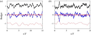
The fact that the systems have indeed reached a statistically stationary state has been determined by monitoring various statistical quantities of both phases, some of which will be discussed below (e.g. the kinetic energy budget shown in figure 1 and the Voronoï tessellation of the disperse phase in figure 7), others not being shown here (e.g. the longitudinal velocity derivative skewness).
Time evolution of the terms in the equation for kinetic energy
 $E_{k}=\boldsymbol{u}\boldsymbol{\cdot }\boldsymbol{u}/2$
, averaged over the computational domain: (a) case D5; (b) case D11. As shown by Chouippe & Uhlmann (Reference Chouippe and Uhlmann2015) the evolution equation reads as follows:
 $0=-\text{d}\langle E_{k}\rangle _{\unicode[STIX]{x1D6FA}}/\text{d}t-\unicode[STIX]{x1D700}_{\unicode[STIX]{x1D6FA}}+\unicode[STIX]{x1D6F9}^{(t)}+\unicode[STIX]{x1D6F9}^{(p)}$
, where
 $\langle \cdot \rangle _{\unicode[STIX]{x1D6FA}}$
indicates averaging over the spatial domain,
 $\unicode[STIX]{x1D700}_{\unicode[STIX]{x1D6FA}}$
is the box-averaged instantaneous dissipation rate (- - -, red),
 $\unicode[STIX]{x1D6F9}^{(t)}$
the power input due to turbulence forcing (——, black), and
 $\unicode[STIX]{x1D6F9}^{(p)}$
the two-way coupling term (——, red); the time-rate-of-change term is plotted in blue (——, blue).

3 Results
3.1 Basic Eulerian and Lagrangian statistics
Figure 1 shows the time evolution of the terms in the budget of the kinetic energy when averaging over the entire computational domain (cf. Chouippe & Uhlmann Reference Chouippe and Uhlmann2015). In both cases the turbulence-forcing power input is, on time average, balanced by the dissipation rate, while the two-way coupling term does not play a significant role (its time-average value corresponds to
 $0.004$
and
 $0.016$
times that of the dissipation rate in case D5 and D11, respectively). The instantaneous imbalance between power input and dissipation leads to temporal fluctuations of the turbulent kinetic energy, whose temporal variance, however, is smaller than 8.5 % in both cases.
Even though the direct effect of the presence of solid particles through the two-way coupling term is practically negligible, the presence of the particles might still have an important impact upon the flow. In the present configurations the comparison between particle-laden and unladen flows shows that this is not the case. In particular, the time-averaged turbulent kinetic energy is only slightly reduced to
 $k=0.99k_{SP}$
(where the subscript ‘SP’ refers to the corresponding single-phase simulation) in both cases, while the value of the time-averaged dissipation rate either mildly increases (
 $\unicode[STIX]{x1D700}=1.03\unicode[STIX]{x1D700}_{SP}$
in case D5) or slightly decreases (
 $\unicode[STIX]{x1D700}=0.99\unicode[STIX]{x1D700}_{SP}$
in case D11). As a result, the obtained Taylor-scale Reynolds numbers in the present particulate flow simulations are mildly different from the unladen counterparts:
 $Re_{\unicode[STIX]{x1D706}}/Re_{\unicode[STIX]{x1D706}}^{(SP)}=0.98$
in case D5, and
 $Re_{\unicode[STIX]{x1D706}}/Re_{\unicode[STIX]{x1D706}}^{(SP)}=0.99$
in case D11. As a conclusion of this short analysis of the global flow quantities we can state that the addition of particles at the current parameter points does not induce a significant modification of the carrier flow, except possibly locally in the vicinity of the particles. This statement will be further corroborated by the following analysis. Note that an investigation of the mechanisms of particle-induced turbulence attenuation is outside the present scope, and the reader is referred to Lucci et al. (Reference Lucci, Ferrante and Elghobashi2010, Reference Lucci, Ferrante and Elghobashi2011) for a detailed discussion in the context of finite-size particles suspended in decaying homogeneous-isotropic turbulence.
The velocity field in homogeneous-isotropic turbulence is well known to be nearly Gaussian distributed, with a slightly sub-Gaussian flatness (Jiménez Reference Jiménez1998; Wilczek, Daitche & Friedrich Reference Wilczek, Daitche and Friedrich2011). We observe the same distribution for the fluid velocity in the particulate case, the flatness measuring
 $2.89$
at both presently investigated parameter points (figure omitted). The one-component p.d.f. of particle velocity (figure omitted) is also found to be close to a Gaussian distribution, with a flatness measuring
 $2.84$
(
 $2.82$
) in case D5 (D11). This result is consistent with the observations of previous authors in similar flow configurations at roughly comparable parameter points (Homann & Bec Reference Homann and Bec2010; Yeo et al.
Reference Yeo, Dong, Climent and Maxey2010).
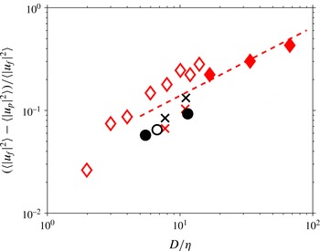
Normalized difference between the variance of the fluid velocity and that of the particle velocity. The symbols correspond to: ♢, Homann & Bec (Reference Homann and Bec2010); ♦, Cisse (Reference Cisse2015); (
 $\times$
, red), density-matched particles (cases ‘N1’, ‘N2’) of Yeo et al. (Reference Yeo, Dong, Climent and Maxey2010); (
 $\times$
, black), particles with density ratio
 $\unicode[STIX]{x1D70C}_{p}/\unicode[STIX]{x1D70C}_{f}=1.4$
(cases ‘S1’, ‘S2’) of Yeo et al. (Reference Yeo, Dong, Climent and Maxey2010); ●, present simulations; ○, case ‘A-G0’ from Chouippe & Uhlmann (Reference Chouippe and Uhlmann2015). The dashed line (- - -) indicates a power law proportional to
 $(D/\unicode[STIX]{x1D702})^{2/3}$
.

Let us turn to the variance of the velocities, which can be conveniently discussed in terms of the relative difference between the value of the fluid phase and the one of the particle phase, viz.
 $(\langle |\boldsymbol{u}_{f}|^{2}\rangle -\langle |\boldsymbol{u}_{p}|^{2}\rangle )/\langle |\boldsymbol{u}_{f}|^{2}\rangle$
. It is clear that the tracer limit corresponds to a vanishing difference, and it can be expected that the value increases with particle size. Homann & Bec (Reference Homann and Bec2010) have shown that the difference of the velocity variance roughly follows a
 $D^{2/3}$
power law for sufficiently large particle diameters, approximately for
 $D/\unicode[STIX]{x1D702}\gtrsim 5$
. As remarked by these authors, dimensional arguments in the inertial range indeed suggest such a dependency. Note that this scaling implies the following assumptions: (i) an inertial range exists (i.e. sufficiently large Reynolds number
 $Re_{\unicode[STIX]{x1D706}}$
); (ii) supposing that the particle velocity is determined by flow scales of size equal to or larger than the particle diameter. Figure 2 shows that although assumption (i) is not completely fulfilled by the numerical simulations, such a power law is found to be consistent with the data of Homann & Bec (Reference Homann and Bec2010) and the more recent data of Cisse (Reference Cisse2015) (performed at larger Reynolds number). The
 $2/3$
power law also roughly matches the variation of the difference of velocity variance measured in the simulations of Yeo et al. (Reference Yeo, Dong, Climent and Maxey2010), which feature an ensemble of particles, in both density-matched and non-density-matched cases (with a density ratio of
 $\unicode[STIX]{x1D70C}_{p}/\unicode[STIX]{x1D70C}_{f}=1.4$
). In the latter case it was observed that the mild excess of particle density has the tendency to increase the difference of velocity variances somewhat – as might be expected from the enhanced particle inertia. The present data set, together with case A-G0 of Chouippe & Uhlmann (Reference Chouippe and Uhlmann2015), adds three data points to figure 2. It can be seen that our present results are consistent with the power law proposed by Homann & Bec (Reference Homann and Bec2010) for particles with diameter
 $D/\unicode[STIX]{x1D702}\gtrsim 3$
. It should be noted that the difference of velocity variances at small particle diameters (particularly in case D5) is a very small quantity compared to the velocity variances themselves, which makes it sensitive to statistical sampling errors. This underlines the necessity to consider observation intervals which are large multiples of the large-eddy time scales.
A quantity of considerable interest for the purpose of modelling the particle motion (e.g. in the context of a point-particle approach) is the relative velocity between the two phases. Note that even the definition of a relevant fluid velocity in the vicinity of the particles (or equivalently a fluid velocity ‘seen’ by the particles) is a matter of debate, and various alternative expressions have been proposed (Bagchi & Balachandar Reference Bagchi and Balachandar2003; Lucci et al.
Reference Lucci, Ferrante and Elghobashi2010; Klein et al.
Reference Klein, Gibert, Bérut and Bodenschatz2012; Cisse et al.
Reference Cisse, Homann and Bec2013; Kidanemariam et al.
Reference Kidanemariam, Chan-Braun, Doychev and Uhlmann2013; Uhlmann & Doychev Reference Uhlmann and Doychev2014). Here we proceed as in Uhlmann & Doychev (Reference Uhlmann and Doychev2014), and define the fluid velocity seen by the
 $i$
th particle,
 $\boldsymbol{u}_{f}^{(i)}$
, by computing an average of the fluid velocity over the surface of a sphere with diameter
 $D_{S}$
, centred at the
 $i$
th particle’s centre location. Recall that the averaging diameter should neither be too small (in which case the fluid velocity will tend to the particle velocity as the no-slip boundary is approached) nor too large (in which case the resulting fluid velocity will no longer be relevant to the motion of the particle under consideration). Based upon our previous work (Kidanemariam et al.
Reference Kidanemariam, Chan-Braun, Doychev and Uhlmann2013) we have chosen the averaging diameter as
 $D_{S}=3D$
throughout the present study. We can then compute a relative velocity
 $\boldsymbol{u}_{pr}^{(i)}=\boldsymbol{u}_{p}^{(i)}-\boldsymbol{u}_{f}^{(i)}$
from which we define an instantaneous particle Reynolds number
 $Re_{p}^{(i)}(t)=|\boldsymbol{u}_{pr}^{(i)}|D/\unicode[STIX]{x1D708}$
. Note that the probability distributions of the components of the relative velocity
 $\boldsymbol{u}_{pr}^{(i)}$
(figure omitted) feature exponential tails. The p.d.f. of the particle Reynolds number
 $Re_{p}$
(normalized to variance unity) is then found to be close to a gamma distribution with shape parameter
 $k=3$
, as shown in figure 3. The match is particularly good in case D5, except for extremely large values of
 $Re_{p}$
, where the p.d.f. is somewhat wider than the tail of the gamma distribution (the flatness measures
 $5.9$
, while the flatness is equal to
 $5$
for the gamma distribution). Case D11, on the other hand, exhibits a slightly narrower shape with a flatness of
 $4.69$
. The mean and variance of the particle Reynolds number recorded in the two cases are also listed in figure 3. They demonstrate that appreciable values of
 $Re_{p}$
can be attained instantaneously, although the particle sizes are still relatively small and the Stokes numbers are not enormously high. In fact, the particle Reynolds numbers are sufficient for the formation of attached vortical structures in the vicinity of the particles, as will be further discussed in § 3.3. These findings suggest that a quasi-steady linear drag assumption would not be appropriate when modelling the hydrodynamic force in the framework of a point-particle model in the present parameter range. We have checked the sensitivity of these results with respect to the choice of the averaging diameter
 $D_{S}$
: going from
 $D_{S}=2.75D$
to
 $D_{S}=3.25D$
increases the mean particle Reynolds number from
 $6.8$
to
 $9.0$
(
 $29.8$
–
 $34.4$
) in case D5 (D11).
Normalized p.d.f. of the particle Reynolds number computed from the sphere-averaged relative velocity
 $\boldsymbol{u}_{pr}$
as defined in the text. Line styles correspond to: (


 $k=3$
which for a quantity
 $x$
with variance unity reads:
 $f(x)=(3^{3/2}/2)x^{2}\exp (-x\sqrt{3})$
. Mean and standard deviations of the particle Reynolds number are listed next to the graph.

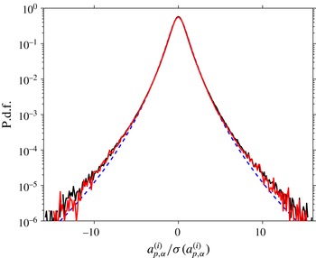
Normalized p.d.f.s of the linear particle acceleration. Samples corresponding to particles in contact with other particles have been eliminated. Line styles correspond to: (——, black), case D5; (——, red), case D11; (- - -, blue), fit of experimental data proposed by Qureshi et al. (Reference Qureshi, Bourgoin, Baudet, Cartellier and Gagne2007).

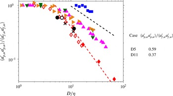
Variance of the single-component particle acceleration normalized by the variance of fluid particles, plotted as function of the particle diameter. The present data are represented by the filled circular symbols (●); additionally, numerical values are listed next to the graph. The open circle (○) indicates the case ‘A-G0’ from Chouippe & Uhlmann (Reference Chouippe and Uhlmann2015). The dark green triangles (▾) mark the experimental results of Voth et al. (Reference Voth, la Porta, Crawford, Alexander and Bodenschatz2002) which were obtained in a von Kármán flow at different Reynolds numbers (
 $Re_{\unicode[STIX]{x1D706}}=140,\ldots ,970$
). The orange triangles (▸) indicate the more recent measurements in the same flow, carried out at Reynolds numbers
 $Re_{\unicode[STIX]{x1D706}}=400,\ldots ,800$
, as reported by Brown et al. (Reference Brown, Warhaft and Voth2009). The blue squares (▪) correspond to the wind-tunnel data of Qureshi et al. (Reference Qureshi, Bourgoin, Baudet, Cartellier and Gagne2007) for neutrally buoyant particles at
 $Re_{\unicode[STIX]{x1D706}}=160$
. The magenta triangles (▴) are experimental measurements in a von Kármán flow by Volk et al. (Reference Volk, Calzavarini, Lévêque and Pinton2011), performed at different Reynolds numbers (
 $Re_{\unicode[STIX]{x1D706}}=590,\ldots ,1050$
). Red diamonds represent the simulation data of Homann & Bec (Reference Homann and Bec2010) (♢) and those of Cisse (Reference Cisse2015) (♦). The numerical data for density-matched particles (cases ‘N1’, ‘N2’) of Yeo et al. (Reference Yeo, Dong, Climent and Maxey2010) are indicated by the symbol (
 $\times$
) in red and their particles with density ratio
 $\unicode[STIX]{x1D70C}_{p}/\unicode[STIX]{x1D70C}_{f}=1.4$
(cases ‘S1’, ‘S2’) are shown as (
 $\times$
) in black. The guiding lines are proportional to
 $(D/\unicode[STIX]{x1D702})^{-2/3}$
(- - -, black) and to
 $(D/\unicode[STIX]{x1D702})^{-4/3}$
(- - -, red).

The statistics of particle acceleration are still a matter of debate in the literature. It is now well established that the normalized p.d.f. of the linear particle acceleration has a nearly universal shape as proposed by Mordant et al. (Reference Mordant, Crawford and Bodenschatz2004) and fitted to an experimental data set with a wide range of parameters by Qureshi et al. (Reference Qureshi, Bourgoin, Baudet, Cartellier and Gagne2007). The data corresponding to the two present simulations in figure 4 nearly overlap, and they are indeed very well represented by the empirical formula of these latter authors, although some deviation in the extreme tails leads to a somewhat larger flatness of
 $10.58$
(
 $9.86$
) in case D5 (D11) as compared to the original empirically fitted value of
 $8.37$
. Turning now to the variance of particle acceleration, the appropriate scaling with particle size is not clear to date. The data from von Kármán flow experiments by Voth et al. (Reference Voth, la Porta, Crawford, Alexander and Bodenschatz2002), Brown et al. (Reference Brown, Warhaft and Voth2009) and Volk et al. (Reference Volk, Calzavarini, Lévêque and Pinton2011), as well as the wind-tunnel data of Qureshi et al. (Reference Qureshi, Bourgoin, Baudet, Cartellier and Gagne2007) suggest a
 $(D/\unicode[STIX]{x1D702})^{-2/3}$
power law for particle diameters exceeding a few multiples of the Kolmogorov length. Such a power law can be inferred from classical Kolmogorov inertial-range arguments, supposing that the particle acceleration will be principally determined by flow scales of the order of the particle diameter. Volk et al. (Reference Volk, Calzavarini, Lévêque and Pinton2011) have refined the analysis and suggested an intermittency correction which accounts for the slightly steeper slope (of
 $D^{-0.81}$
) in their measurements. Figure 5 shows the particle acceleration variance normalized by the fluid counterpart, which allows the comparison of data measured at different Reynolds numbers (cf. Vedula & Yeung (Reference Vedula and Yeung1999), Voth et al. (Reference Voth, la Porta, Crawford, Alexander and Bodenschatz2002) for the scaling of the fluid acceleration variance with Reynolds number). On the other hand, the normalized particle acceleration variance from the DNS of Homann & Bec (Reference Homann and Bec2010) (performed at
 $Re_{\unicode[STIX]{x1D706}}=32$
) and Cisse (Reference Cisse2015) (
 $Re_{\unicode[STIX]{x1D706}}=160$
) approximately follows a
 $(D/\unicode[STIX]{x1D702})^{-4/3}$
trend. Homann & Bec (Reference Homann and Bec2010) argue that at low Reynolds numbers the predominant mechanism affecting the particle motion is sweeping by the large scales, which might explain the different scaling. Now let us consider the particle acceleration variance obtained in the present simulations. Recall that the principal difference with respect to the previously mentioned experiments and simulations is the fact that the present particles are not density matched. It can be seen from figure 5 that the results for case D5 and D11, as well as the one for case A-G0 of Chouippe & Uhlmann (Reference Chouippe and Uhlmann2015) are consistent with the results of Homann & Bec (Reference Homann and Bec2010) and Cisse (Reference Cisse2015) to within the scatter of the available reference data points. This observation suggests that the effect of a mild excess particle density (
 $\unicode[STIX]{x1D70C}_{p}/\unicode[STIX]{x1D70C}_{f}=1.5$
) as well as the collective effects in the present dilute regime (
 $\unicode[STIX]{x1D6F7}_{s}=0.005$
) do not have a significant impact upon the particle acceleration variance in the absence of gravity. The data set of Yeo et al. (Reference Yeo, Dong, Climent and Maxey2010), which features parameters comparable to our present simulations, allows us to discuss the specific impact of the particle-to-fluid density ratio upon the particle acceleration variance. It should be noted that the authors have estimated the fluid acceleration variance from the value provided by Yeung & Pope (Reference Yeung and Pope1989) in a separate single-phase simulation at the same Reynolds number. These data points are included in the present figure 5; however, they should probably be treated with some caution. It can be seen that increasing the particle density from the density-matched value by a factor of
 $1.4$
does not have a very large effect in the work of Yeo et al. (Reference Yeo, Dong, Climent and Maxey2010). Both data points (for
 $D/\unicode[STIX]{x1D702}=7.7$
and
 $11$
) are shifted by approximately the same fraction downward, i.e. increasing density decreases the acceleration variance, as can be expected. Note that the ratio between the value for
 $\unicode[STIX]{x1D70C}_{p}/\unicode[STIX]{x1D70C}_{f}=1.4$
and for the density-matched counterparts amounts to approximately
 $0.8$
(for both particle diameters), which is substantially larger than what might be expected when directly applying the factor due to the density ratio, i.e.
 $(\unicode[STIX]{x1D70C}_{p}/\unicode[STIX]{x1D70C}_{f})^{-2}\approx 0.51$
, which enters through the Newton–Euler equation for particle motion. As a conclusion of this short discussion of density effects, it can be stated that according to the work of Yeo et al. (Reference Yeo, Dong, Climent and Maxey2010) the variance of particle acceleration varies more slowly than inversely proportional to the solid-to-fluid density ratio. It should also be pointed out that Qureshi et al. (Reference Qureshi, Arrieta, Baudet, Cartellier, Gagne and Bourgoin2008) have revealed intricate effects of particle density upon the acceleration variance; however, their laboratory measurements were performed in the presence of non-zero gravitational acceleration, and, therefore, a direct comparison with the present data does not seem pertinent.
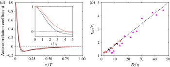
As a final point in this section we wish to discuss the Lagrangian auto-correlation of particle acceleration. This quantity provides the information on the time scales over which particles are accelerated, which was so far missing from the above discussion. Figure 6(a) shows the data in both large-eddy scaling and Kolmogorov scaling. It can be seen that the long-time behaviour of both present cases nearly overlaps, with a negative loop and a gradual approach to zero from below on the order of one large-eddy turnover time. The short-time behaviour, i.e. the first zero-crossing time scale, on the contrary, increases with particle diameter. Let us define an integral time scale
 $\unicode[STIX]{x1D70F}_{int}$
by integration of the auto-correlation coefficient up to the time of the first zero crossing. Figure 6(b) shows the variation of
 $\unicode[STIX]{x1D70F}_{int}$
as a function of the particle diameter, both axes being normalized with Kolmogorov scales. The data for cases D5, D11 and case A-G0 of Chouippe & Uhlmann (Reference Chouippe and Uhlmann2015) are obviously well represented by a linear variation
 $\unicode[STIX]{x1D70F}_{int}/\unicode[STIX]{x1D70F}_{\unicode[STIX]{x1D702}}=1+0.08(D/\unicode[STIX]{x1D702})$
. The same is true for the DNS results of Homann & Bec (Reference Homann and Bec2010), and – with some scatter – for the experimental data of Volk et al. (Reference Volk, Calzavarini, Lévêque and Pinton2011). However, as remarked by Volk et al. (Reference Volk, Calzavarini, Lévêque and Pinton2011), over the limited range of particle sizes one cannot definitely exclude an alternative scaling with
 $(D/\unicode[STIX]{x1D702})^{2/3}$
, as implied by classical Kolmogorov inertial-range arguments. The main conclusion from the present data is the insensitivity of the Lagrangian time scales which characterize the particle acceleration, i.e. the hydrodynamic forces, with respect to mild variations of the density ratio.
(a) Lagrangian auto-correlation coefficient of one-component, linear particle acceleration, normalized with the large-eddy turnover time
 $T$
. The correlations have been computed during collision-free intervals only. The inset shows the same data for smaller separation times
 $\unicode[STIX]{x1D70F}$
, and normalized in Kolmogorov time units
 $\unicode[STIX]{x1D70F}_{\unicode[STIX]{x1D702}}$
. Line styles correspond to: (——, black), case D5; (——, red), case D11, (b) The integral scale
 $\unicode[STIX]{x1D70F}_{int}$
of the auto-correlation (from integration up to the first zero crossing) shown in (a), plotted as a function of the particle size. The present data is indicated by solid circles (●); the black open circle (○) indicates the data of case ‘A-G0’ from Chouippe & Uhlmann (Reference Chouippe and Uhlmann2015). The magenta triangles (▴) correspond to data from the von Kármán flow experiments of Volk et al. (Reference Volk, Calzavarini, Lévêque and Pinton2011); the red diamonds (♢) represent the simulation data of Homann & Bec (Reference Homann and Bec2010). The dashed line (- - -) indicates a linear increase
 $\unicode[STIX]{x1D70F}_{int}/\unicode[STIX]{x1D70F}_{\unicode[STIX]{x1D702}}=1+0.08(D/\unicode[STIX]{x1D702})$
.

(a) Time evolution of the standard deviation of the normalized volume of the cells of the three-dimensional Voronoï tessellation with the particle centres as ‘sites’. Line styles correspond to: (


3.2 Particle clustering
Voronoï tessellation is a computationally efficient means for the analysis of the spatial structure of the dispersed phase (Monchaux, Bourgoin & Cartellier Reference Monchaux, Bourgoin and Cartellier2010; Monchaux et al. Reference Monchaux, Bourgoin and Cartellier2012). In the context of particulate flow, one typically takes the particle centres as the sites for which a three-dimensional partition of space into cells is performed such that each point in a given cell is located closer to the cell’s site than to any other site. The inverse of the volume of a Voronoï cell is then a measure of the local concentration: a smaller cell corresponds to a denser particle arrangement and vice versa. Particle positions drawn at random (from a random Poisson process) yield Voronoï cell volumes which (when normalized with the mean cell volume) exhibit a universal p.d.f. given by a gamma distribution with parameters determined numerically by Ferenc & Neda (Reference Ferenc and Neda2007). When considering finite-size particles, this result is no longer valid, since particles should not overlap. Therefore, the parameters of the random distribution need to be computed specifically for each given solid volume fraction and box size. It turns out that the data for the Voronoï cell volumes of the real particle phase is also gamma distributed, however with a different variance: those cases which exhibit ‘clustering’ feature a larger variance than the random data (cf. Monchaux et al. Reference Monchaux, Bourgoin and Cartellier2012; Uhlmann & Doychev Reference Uhlmann and Doychev2014). This suggests that the variance of the normalized Voronoï cell volumes can be taken as a single indicator of particle ‘clustering’, i.e. of a particle arrangement which is statistically distinct from that obtained by a random Poisson process in the sense that it features more closely located particles and more voids than the latter. Figure 7(a) shows the time evolution of the variance of Voronoï cell volumes in the two present cases. Also marked are the averages of the random data computed from a large ensemble for the present solid volume fraction and the two box sizes. It can be seen that the variance in both cases D5 and D11 is clearly above the random value. It is also obvious that the same quantity fluctuates more in time in case D11 which features an eight times smaller number of particles. In figure 7(b) we report the time average of the instantaneous variance of Voronoï cell volumes, normalized by their respective average random value, along with their temporal standard deviation (in form of error bars). It is clearly visible that the particle phase in case D5 exhibits stronger clustering than in case D11 with values of the variance which are 7.7 % and 3.1 % larger than the random value, respectively. It should be noted that this clustering behaviour can be qualified as relatively weak. For comparison, in the clustering case of Uhlmann & Doychev (Reference Uhlmann and Doychev2014) the variance was approximately 50 % larger than the random value.
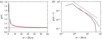
An alternative way of characterizing a spatial distribution of a set of points which is often employed in the context of particulate flow is the RDF, i.e. the probability of finding a second particle at a given distance of a test particle. Figure 8 shows the normalized RDF for both cases D5 and D11 in linear and logarithmic scaling. This quantity confirms that the clustering is more pronounced in case D5 than D11. The decay with distance
 $r$
from the test particle is found to follow a power law with an approximate scaling as
 $r^{-1}$
for
 $r\lesssim 20\unicode[STIX]{x1D702}$
.
(a) Normalized radial-distribution function
 $g(r)$
of particle positions in case D5 (——, black) and D11 (——, red) in the statistically stationary regime. (b) The same data as in (a), but showing the excess value
 $g(r)-1$
in double-logarithmic scaling. The blue dashed line (- - -) corresponds to a
 $-1$
power law.

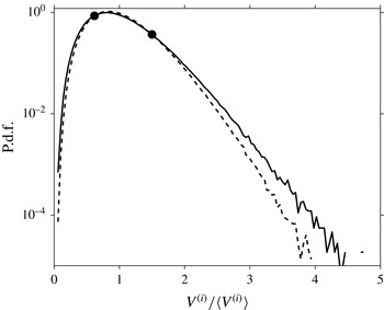
P.d.f. of the Voronoï cell volumes, sampled over the entire statistically stationary interval in case D5 (——), as compared with the distribution obtained from a random Poisson process (- - -), sampled over a large ensemble. The cross-over points between the two curves are marked with solid circles (●).

The Voronoï data can be utilized to define a host of additional diagnostic quantities (Monchaux et al.
Reference Monchaux, Bourgoin and Cartellier2010). One of them is the objective definition of a cluster. As can be seen in figure 9, the fact that the variance in the DNS data is larger than the corresponding random particle arrangement leads to a cross-over between the two p.d.f.s. The two cross-over points (marked in the figure) can then be used as objective thresholds for defining clusters and void areas. Here it is found that the lower cross-over point measures
 $0.62$
times the average Voronoï cell volume in case D5. Note that this threshold is equivalent to 124 times the particle volume
 $V_{p}$
(as compared to
 $200V_{p}$
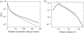
for the mean volume), which is still far from a dense particle arrangement. Monchaux et al. (Reference Monchaux, Bourgoin and Cartellier2010) propose that all those particles belong to a cluster whose associated cell has a Voronoï cell volume smaller than the one given by the lower cross-over point. This information can e.g. be used to track the residence time of particles in a given cluster (Uhlmann & Doychev Reference Uhlmann and Doychev2014). Here we attempt to extract information on the cluster size in terms of the number of members per cluster. For this purpose a cluster is constructed in the spirit of Monchaux et al. (Reference Monchaux, Bourgoin and Cartellier2010) by first marking all Voronoï cells according to the lower volume threshold, then connecting those which share at least one vertex of their respective Voronoï cells. For each instant in time this leads to a set of clusters with a number of individual cells (each associated with a single particle) as members. Figure 10(a) shows the p.d.f. of the cluster size computed over the statistically stationary time interval. In comparison to the data for an artificial particle arrangement drawn from a random Poisson process the DNS data set clearly exhibits a significantly higher number of very large clusters, i.e. much more marked tails in the p.d.f. Additionally, we have computed the volume of each detected cluster as the sum of the members’ Voronoï cells, and figure 10(b) shows the corresponding p.d.f. in log–log scaling. It can be seen that the cluster volume distribution features a peak at approximately
 $10^{4}\unicode[STIX]{x1D702}^{3}$
, an approximate power-law decay over a range of nearly two decades, and an exponential decay for the largest volumes. The most probable cluster size corresponds to a linear dimension of approximately
 $20\unicode[STIX]{x1D702}$
which is somewhat larger than, but comparable to the experimental results of Aliseda et al. (Reference Aliseda, Cartellier, Hainaux and Lasheras2002) and Obligado et al. (Reference Obligado, Teitelbaum, Cartellier, Mininni and Bourgoin2014) for sub-Kolmogorov-size particles, both determined from planar measurements. Goto & Vassilicos (Reference Goto and Vassilicos2006) have proposed a model for the statistical distribution of the area of the voids in a point-particle arrangement in forced two-dimensional turbulence. Their model is based upon the assumptions of a fully developed Kolmogorov inertial range and upon a one-to-one correspondence between the ‘holes’ in the particle field and the size of the fluid eddies from which particles are ejected; this leads to a
 $-5/3$
power-law over the range of scales affecting the particle motion. The model predictions have recently been confirmed by Sumbekova et al. (Reference Sumbekova, Cartellier, Aliseda and Bourgoin2016) based upon their laboratory measurements of small-particle data in active-grid turbulence in a wind tunnel. These latter authors have also observed that the same power-law scaling as the one for the voids applies to the areas occupied by the clusters themselves. When applying the model assumptions of Goto & Vassilicos (Reference Goto and Vassilicos2006) to the volume of the structures in a three-dimensional flow (instead of the area) one obtains an exponent of
 $-16/9$
, which is not too far from what is presently observed, as can bee seen in figure 10(b). However, since the flow Reynolds number is not very large here, the extent of the inertial range is rather limited.
(a) P.d.f. of the size distribution of particle clusters expressed in terms of the number of member cells per cluster. The black solid line (——) corresponds to case D5; the dashed line (- - -, black) shows the distribution for a corresponding random particle arrangement. (b) P.d.f. of the distribution of the volume of particle clusters. The dashed line (- - -, blue) corresponds to a
 $-16/9$
power-law.

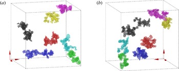
A visualization of the largest clusters in a snapshot of simulation D5 is shown in figure 11. It can be observed that the large clusters feature an irregular shape which can neither be described as filamentary nor as compact. A more detailed investigation of the geometrical properties of the clusters, however, has not been attempted at the current time.
The seven largest clusters in some snapshots of case D5, with the Voronoï cell faces coloured uniformly per cluster. The colour code is in descending order (the number of member cells is given in parenthesis): black (90), blue (80), red (77), magenta (76), green (64), cyan (59) and yellow (56). The particles inside those cells are coloured in black, while all remaining particles have been omitted from the figure. Graphs (a) and (b) show the same data from two different perspectives.

3.3 Preferential particle locations
The preceding section (in particular figure 7 b) has shown that the solid phase is not randomly distributed in space; instead it features a mild level of clustering. In the absence of gravity and considering the low value of the global solid volume fraction in the present simulations, it is clear that this effect is not a consequence of collective particle dynamics, but that it is directly induced by the turbulent background flow. The question is then: which mechanism is responsible for the formation of the statistically significant excess of clusters in the case of suspended finite-size particles? In the following we will consider two of the principal mechanisms which have been proposed in the context of sub-Kolmogorov particles, as discussed in the introduction, i.e. the centrifugal effect (Maxey Reference Maxey1987) and the sweep-stick mechanism (Goto & Vassilicos Reference Goto and Vassilicos2008).
Let us first consider the centrifugal effect. It hinges upon the rotational property of the fluid motion and the conditions that: (i) the particle inertia is sufficiently large such that particle paths deviate from fluid particle paths and (ii) the excess inertia still does not place the particles in the ballistic regime. In the context of the simplest point-particle assumption, the argument then boils down to a comparison of time scales, viz. considering the value of the Stokes number. Now in the case of finite-size particles it is doubtful that the Stokes number alone is a sufficient parameter to predict clustering, as has been demonstrated by Fiabane et al. (Reference Fiabane, Zimmermann, Volk, Pinton and Bourgoin2012). On the other hand, an analysis of the role of coherent vortices upon the motion of particles with a diameter comparable to or larger than the Kolmogorov length has to our knowledge previously not been undertaken.
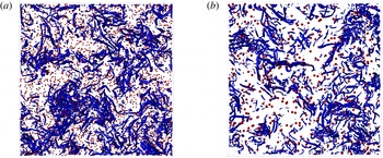
Snapshot of the flow field and the particle positions in cases (a) D5; (b) D11. Intense vortical structures are educed with the
 $q$
-criterion of Hunt, Wray & Moin (Reference Hunt, Wray and Moin1988), and locations with a value of
 $1.5$
times the standard deviation of
 $q$
are shown as blue coloured surfaces. Only a slice with thickness equal to one-eighth of the domain size (equivalent to approximately
 $90$
Kolmogorov units) is shown for clarity; in the other two directions the entire domain is shown.

As a first step in this direction we educe the coherent vortical structures with the aid of the ‘
 $q$
-criterion’ of Hunt et al. (Reference Hunt, Wray and Moin1988). Denoting by ‘
 $q$
’ the second invariant of the velocity gradient tensor (
 $q=u_{i,i}^{2}/2-u_{i,j}u_{j,i}/2$
), we define an intense vortical region as one where a given threshold value of this quantity is exceeded, viz.
 $q>q_{thresh}=1.5\unicode[STIX]{x1D70E}_{q}$
(where
 $\unicode[STIX]{x1D70E}_{q}$
is the standard deviation of
 $q$
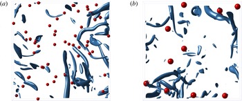
). Figure 12 gives an impression of the typical worm-like structures which are educed with this method in conjunction with the relative locations of particles, while a close up of the same data is provided in figure 13. Globally the visualization looks similar to the single-phase counterpart (not shown), featuring elongated vortices with a diameter of several Kolmogorov lengths, as previously observed by many authors (e.g. She, Jackson & Orszag Reference She, Jackson and Orszag1990; Jiménez et al.
Reference Jiménez, Wray, Saffman and Rogallo1993; Moisy & Jiménez Reference Moisy and Jiménez2004). Close inspection of the present images reveals, however, that a relatively large fraction of the particles is accompanied by small vortices in their vicinity. This is expected in the present cases, since the particle Reynolds number based upon the instantaneous relative velocity reaches substantial values (cf. figure 3) such that the formation of small transient wakes occurs frequently. In order to gain quantitative insight into the geometry of the educed vortices, we have computed the volume enclosed by each individual ‘worm’. After determining a triangulation of the surface defined by
 $q=q_{thresh}$
, we compute the enclosed volume from a surface integral (making use of the divergence theorem); this procedure is repeated for a number of flow fields in order to accumulate significant statistics. The resulting probability distribution of the ‘worm’ volumes is shown in figure 14. It can be seen that the distribution in case D11 is essentially identical to the single-phase data. Case D5 on the other hand features a larger number of small-volume vortical structures than the single-phase data, the rise being observed for volumes smaller than approximately one-half of the particle volume
 $V_{p}=D^{3}\unicode[STIX]{x03C0}/6$
. Due to the normalization of the p.d.f., the curve corresponding to case D5 is then slightly shifted downward (as compared to single-phase data) at larger volumes. In absolute terms, however, the occurrence of vortical structures with a volume comparable to and larger than the particle volume are also essentially the same in case D5 as in the single-phase data set. This discussion shows that the presence of the finite-size particles in both present simulations only affects the number density of small structures with a volume smaller than the particle volume. The fact that this feature is much more pronounced in case D5 can be explained with the larger number density of particles (by a factor of 8) as compared to case D11. Note that Moisy & Jiménez (Reference Moisy and Jiménez2004) have performed an analysis of the volume distribution of intense vortices in single-phase homogeneous-isotropic turbulence. Although their definition of a ‘worm’ is slightly different (i.e. based upon the magnitude of the vorticity field), we observe a good qualitative agreement when choosing a similar objective threshold value.
The same data as in figure 12, but showing a close up with side length equal to
 $180\unicode[STIX]{x1D702}$
and a reduced depth of
 $45\unicode[STIX]{x1D702}$
.

The p.d.f. of the volume of the vortical structures, educed with the criterion of Hunt et al. (Reference Hunt, Wray and Moin1988) (using a threshold equal to
 $1.5$
times the standard deviation) and normalized in Kolmogorov length scales. Line styles correspond to: (


 $\unicode[STIX]{x0394}x^{3}$
in each case.

Next we proceed to the characterization of the particle locations with respect to the coherent vortices educed by the method presented in the previous paragraph. Here we again use the information provided by the surface triangulation of the ‘worms’. More specifically, at a given instant in time we determine for the
 $i$
th particle the smallest distance
 $d_{CS}^{(i)}$
from the particle surface to any vertex point of the triangulation of any ‘worm’ surface. The principal quantity of interest is the distribution of the set of so-defined minimum distances
 $d_{CS}^{(i)}$
, but in this fashion we also obtain the identification of the nearest coherent vortex, which gives us access to all its properties. This additional information will be used below in order to further refine the analysis. Figure 15 shows the resulting p.d.f. of the distance
 $d_{CS}^{(i)}$
in case D5, accumulated over the set of particles and over a number of snapshots. As a reference the graph also includes the data corresponding to a set of points which were distributed in the flow fields of case D5 by means of a random Poisson process. Note that the random-point data, which feature an essentially flat distribution that decays exponentially for large distances (
 $d_{CS}^{(i)}\gtrsim 10\unicode[STIX]{x1D702}$
), solely reflect the geometry of the ‘worms’ themselves. By comparison, the finite-size particle DNS data in case D5 exhibit a distinct distribution, namely featuring a marked dip at distances around the Kolmogorov scale and a dominant peak when the distance goes to zero. This result clearly corresponds to a high probability of a vortical structure being practically attached to a particle. The fact that the particles in case D5 induce a substantial amount of small-scale vortical structures (cf. figure 14) suggests that the difference between the random data and the DNS results in figure 15 is actually due to the attached wake structures and not a manifestation of a significant preferential location with respect to coherent structures of the background turbulent flow. In order to remove this bias, we have first eliminated from each snapshot those ‘worms’ that have an enclosed volume smaller than the particle volume. The resulting distribution of the distance to the nearest coherent flow structure is also included in figure 15. It can be seen that filtering the flow field in this manner indeed has the effect that (to within statistical uncertainty) the p.d.f. for the minimum distances measured from the real particles becomes equivalent to the one measured from random points. Therefore, we can conclude from this geometrical analysis that the particles in case D5 do not preferentially accumulate with respect to the intense vortical structures of the turbulent background flow.
P.d.f. of the distance from the particles to the nearest point on any vortical structure (as educed with the criterion of Hunt et al.
Reference Hunt, Wray and Moin1988). Note that the distance
 $d_{CS}^{(i)}$
(defined in the text) is measured from the particle surface. Line styles correspond to:

 $V_{p}$
; ——, blue, distance from randomly chosen points to the coherent structures in case D5.

We now turn to the analysis of the relation between the fluid acceleration field
 $\boldsymbol{a}_{f}$
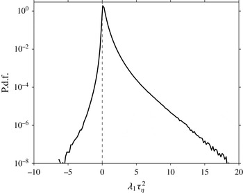
and the particle locations motivated by the results of Goto & Vassilicos (Reference Goto and Vassilicos2008) in the context of sub-Kolmogorov particles. In the framework of the simplest one-way coupled point-particle model (with the hydrodynamic force given by Stokes drag) Goto & Vassilicos (Reference Goto and Vassilicos2008) argue that the particle phase potentially accumulates at points which satisfy the following criterion:
 $$\begin{eqnarray}\displaystyle \boldsymbol{e}_{1}\boldsymbol{\cdot }\boldsymbol{a}_{f}=0,\quad \text{and}\quad \unicode[STIX]{x1D706}_{1}>0. & & \displaystyle\end{eqnarray}$$
In (3.1) the symbol
 $\unicode[STIX]{x1D706}_{1}$
denotes the largest eigenvalue of the symmetric part of the acceleration gradient tensor
 $\unicode[STIX]{x1D63C}\equiv \unicode[STIX]{x1D735}\boldsymbol{a}_{f}+(\unicode[STIX]{x1D735}\boldsymbol{a}_{f})^{\text{T}}$
, and
 $\boldsymbol{e}_{1}$
is the associated eigenvector (normalized to unit length). Recall that the argument relies on the asymptotic result (valid for this point-particle model in the limit of small Stokes number) obtained by Maxey (Reference Maxey1987) which states that the slip velocity is proportional to the fluid acceleration, viz.
 $$\begin{eqnarray}\displaystyle \boldsymbol{u}_{p}-\boldsymbol{u}_{f}\approx -\unicode[STIX]{x1D70F}_{p}\boldsymbol{a}_{f}. & & \displaystyle\end{eqnarray}$$
Taking the divergence of (3.2) then yields the result that the particle ‘field’ should converge wherever the fluid acceleration field diverges (regions where
 $\unicode[STIX]{x1D735}\boldsymbol{\cdot }\boldsymbol{a}_{f}>0$
). Note that the divergence of the fluid acceleration is directly linked to the Laplacian of pressure and to the
 $q$
-criterion of Hunt et al. (Reference Hunt, Wray and Moin1988), viz.
 $\unicode[STIX]{x1D735}\boldsymbol{\cdot }\boldsymbol{a}_{f}=-\unicode[STIX]{x1D6FB}^{2}p/\unicode[STIX]{x1D70C}=-2q$
(Jeong & Hussain Reference Jeong and Hussain1995, p. 76). In order to properly account for the multi-dimensional nature of the acceleration field, Goto & Vassilicos (Reference Goto and Vassilicos2008) propose to selectively consider the most expansive direction
 $\boldsymbol{e}_{1}$
of the fluid acceleration
 $\boldsymbol{a}_{f}$
instead of directly working with zero-acceleration points. Hence they suggest to investigate the points defined in (3.1), to which we will henceforth simply refer as ‘sticky points’. Since this criterion focuses the attention on the first principal axis of the tensor
 $\unicode[STIX]{x1D63C}$
, it is not equivalent to an analysis of points with positive divergence of acceleration, and consequently it is not equivalent to simply analysing points with negative values of
 $q$
(i.e. strain-dominated locations in the sense of Hunt et al.
Reference Hunt, Wray and Moin1988). The DNS data of Goto & Vassilicos (Reference Goto and Vassilicos2008) strongly support this argument with a large accumulation of point particles in the vicinity of the sticky points.
The implications of the sweep-stick mechanism for finite-size particles have not been explored in detail (cf. the final discussion by Qureshi et al.
Reference Qureshi, Arrieta, Baudet, Cartellier, Gagne and Bourgoin2008). As a first step in this direction we characterize the structure of the set of points which verify the criterion (3.1) in our simulations. Note that in practice we have not determined the zeros of the projected acceleration component from a minimization. Instead we have identified grid points at which the value falls below a very small threshold value (
 $\boldsymbol{e}_{1}\boldsymbol{\cdot }\boldsymbol{a}_{f}\leqslant a_{P,thresh}=4\times 10^{-4}\unicode[STIX]{x1D70E}_{a,P}$
, where
 $\unicode[STIX]{x1D70E}_{a,P}$
is the standard deviation of
 $\boldsymbol{e}_{1}\boldsymbol{\cdot }\boldsymbol{a}_{f}$
). We have checked the sensitivity of the following analysis with respect to the choice of the threshold by varying the value of
 $a_{P,thresh}$
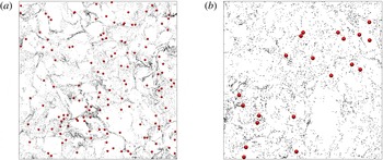
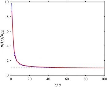
by a factor of four with no visible differences. Figure 16 provides an instantaneous visualization of the set of sticky points in both present particulate flow cases. It can be observed that their spatial distribution is clearly inhomogeneous, featuring a succession of denser filaments, dilute regions and voids. A quantitative measure of the level of clustering in these sets is provided by the radial distribution function, which is computed from a number of flow fields and shown in figure 17. A highly excessive probability of finding sticky points in the immediate vicinity of a given sticky point is observed, which reaches values of the order of ten times the global probability. The decay with distance is found to follow an exponential approach to unity for
 $r/\unicode[STIX]{x1D702}\gtrsim 20$
. Figure 17 also includes the data for single-phase flow, which practically collapse with the curve for the present case D11. This very good agreement between the curves in particulate and single-phase flow implies that the particles do not significantly alter the spatial structure of the set of sticky points, with the consequence that we can consider the latter ones as a quantity pertaining principally to the turbulent background flow.
Instantaneous location of particles (red spheres) and the points of the fluid velocity field (grey dots) which satisfy the criteria of (3.1). The data are shown in a slice of thickness equal to
 $15\unicode[STIX]{x1D702}$
(direction into the page), the length in the other two directions being
 $380\unicode[STIX]{x1D702}$
: (a) case D5; (b) case D11.

Radial-distribution function of ‘sticky points’ as defined in (3.1). The number density
 $n_{S}(r)$
is normalized with the global value
 $n_{SG}$
. The lines correspond to: ——, red, case D11; ——, blue, single-phase flow.

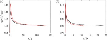
Now we are in a position to characterize the relation between the particle locations and the set of sticky points. For this purpose we have computed the particle-conditioned radial-distribution function of sticky points, i.e. the probability of finding a sticky point at a given distance of a particle. The result is shown in figure 18, where a normalization of the distance in both Kolmogorov units and particle diameter is presented. A statistically significant excess probability is indeed observed in both cases D5 and D11. However, the maximum amplitude of this probability (which occurs at small distances from the test particle) only amounts to approximately 1.1–1.15 times the global probability. This moderate level of statistical correlation between the positions of the particles and those of the sticky points is consistent with the relatively modest amount of clustering exhibited by the former ones (cf. § 3.2). Despite its relatively weak amplitude, the present data clearly link the particle locations to the distribution of the sticky points proposed by Goto & Vassilicos (Reference Goto and Vassilicos2008).
Particle-conditioned, relative number density of ‘sticky points’ (as defined in (3.1)). The number density
 $n_{PS}(r)$
is normalized with the global value
 $n_{PSG}$
. In (a) the distance is scaled with the Kolmogorov length scale
 $\unicode[STIX]{x1D702}$
, in (b) it is scaled with the particle diameter
 $D$
. Line styles: ——, black, case D5; ——, red, case D11.

The work of Coleman & Vassilicos (Reference Coleman and Vassilicos2009) suggests that point particles (under Stokes drag) in homogeneous-isotropic turbulence accumulate preferentially in the vicinity of zero-acceleration points. They conclude that locations identified with this simpler criterion are more strongly correlated with particle clusters than those defined through the projection upon the most expansive eigenvector (i.e. the sticky points given by (3.1)). We have tested this alternative criterion by repeating the previous analysis with respect to zero-acceleration points. Again, the set of ‘zero-acceleration’ points was determined by applying a small threshold (
 $0.05$
times the standard deviation of the fluid acceleration), whose influence on the results has been found to be weak. Figure 19(a) shows a comparison between the particle-conditioned radial-distribution functions of the zero-acceleration points and the previous one pertaining to the sticky points defined by (3.1) in case D5. It can be seen that both criteria lead to very similar results, with a comparable excess probability of roughly 10 % in the direct vicinity of the particles. It can therefore be concluded that the two criteria, (i) zero fluid acceleration, and (ii) zero fluid acceleration projected upon the most expansive direction of the acceleration gradient tensor, feature a comparable statistical correlation with the positions of the present finite-size particles.
(a) Comparison of the particle-conditioned radial-distribution function in case D5 according to different criteria: ——, black, criterion (3.1);


It is also of interest to analyse the influence of the particle size upon the particle-conditioned radial-distribution function of sticky points. Figure 18 shows that scaling the distance in terms of the particle diameter is not appropriate. On the other hand, it can be observed that a normalization in Kolmogorov units leads to a reasonable collapse of the curves for larger distances (
 $r/\unicode[STIX]{x1D702}\gtrsim 50$
). This can be taken as an indication that the level of particle clustering does not influence the far-field decay of the particle-conditioned radial-distribution function too much, where the particles essentially ‘see’ the same sticky-point distribution. Note that in case D11 at small distances from the particle somewhat larger values of the radial-distribution function are recorded than in case D5, although the former case exhibits less intense clustering. Since this effect is restricted to the very near field of the flow around the particle (
 $r/D\lesssim 0.55$
, as obtained from the cross-over coordinate in figure 18
b), it is presumably caused by the difference in the transient wake flows the particles generate as a response to the two respective particle Reynolds number distributions (cf. figure 3).
In order to test whether the correlation between sticky-point locations and particle positions is really relevant for particle clustering, we have additionally computed the radial-distribution function for those particles only which have a Voronoï cell volume smaller than the lower cross-over point in figure 9. The effect of this additional condition upon particle clustering is shown in figure 19(b) for case D5. It can be seen that the restriction to clustering particles leads to significantly larger probabilities of finding a sticky point in the vicinity of the test particle, in particular for distances smaller than approximately
 $10D$
. This additional piece of evidence strongly suggests that there is indeed a causal relationship between the location of sticky points and the tendency of particles to exhibit locally increased levels of concentration.
Finally, let us consider the characteristic time scales of the proposed sweep-stick mechanism. Goto & Vassilicos (Reference Goto and Vassilicos2008) have noted that the values of the largest eigenvalue
 $\unicode[STIX]{x1D706}_{1}$
of the symmetric part of the acceleration gradient tensor are of the order of
 $\unicode[STIX]{x1D70F}_{\unicode[STIX]{x1D702}}^{-2}$
(
 $\unicode[STIX]{x1D70F}_{\unicode[STIX]{x1D702}}$
being the Kolmogorov time scale). Figure 20 shows the probability distribution of
 $\unicode[STIX]{x1D706}_{1}$
in the single-phase case S5. Since we are only concerned with positive values, we have defined the set of points where
 $\unicode[STIX]{x1D706}_{1}>0$
, and denote this quantity
 $\unicode[STIX]{x1D706}_{1}^{+}$
, for which the statistical moments have been determined. It turns out that in the present single-phase case S5 the mean and standard deviation of
 $\unicode[STIX]{x1D706}_{1}^{+}$
measure
 $0.34/\unicode[STIX]{x1D70F}_{\unicode[STIX]{x1D702}}^{2}$
and
 $0.52/\unicode[STIX]{x1D70F}_{\unicode[STIX]{x1D702}}^{2}$
, respectively. Consequently, following Goto & Vassilicos (Reference Goto and Vassilicos2008) one can estimate a characteristic time scale of the compressive effect of the fluid acceleration field as
 $\unicode[STIX]{x1D70F}_{af}=\unicode[STIX]{x1D706}_{1}^{-1/2}$
which indeed turns out to be of the order of the Kolmogorov time scale
 $\unicode[STIX]{x1D70F}_{\unicode[STIX]{x1D702}}$
(e.g. when computing
 $\unicode[STIX]{x1D70F}_{af}$
from the sum of the mean plus one standard deviation of
 $\unicode[STIX]{x1D706}_{1}^{+}$
). This result suggests that the particle Stokes number which would be most susceptible to clustering through the sweep-stick mechanism is of the order of unity when defined with the Kolmogorov time scale, i.e.
 $St_{\unicode[STIX]{x1D702}}=\unicode[STIX]{x1D70F}_{p}/\unicode[STIX]{x1D70F}_{\unicode[STIX]{x1D702}}$
. However, as can be seen in figure 20, the probability distribution of
 $\unicode[STIX]{x1D706}_{1}^{+}$
is very broad, and, consequently, it corresponds to a broad range of time scales, including ones which are much larger than the Kolmogorov time.
P.d.f. of the largest eigenvalue
 $\unicode[STIX]{x1D706}_{1}$
of the symmetric part of the fluid acceleration gradient tensor,
 $\unicode[STIX]{x1D735}\boldsymbol{a}_{f}+(\unicode[STIX]{x1D735}\boldsymbol{a}_{f})^{\text{T}}$
, in single-phase turbulence case S5.

Sumbekova et al. (Reference Sumbekova, Cartellier, Aliseda and Bourgoin2016) have recently argued that the characteristic time scale of the carrier flow in view of preferential accumulation of particles in the vicinity of zero-acceleration points (
 $|\boldsymbol{a}_{f}|=0$
) is expected to be of the order of the Lagrangian correlation time of the magnitude of fluid acceleration. This time scale in turn has been shown to scale with the integral scale (as opposed to the correlation time of individual fluid acceleration components which scale with the Kolmogorov time scale), cf. Mordant et al. (Reference Mordant, Crawford and Bodenschatz2004). This consideration then suggests that from the point of view of time scales the particles can be expected to exhibit some degree of preferential accumulation as long as their time scale does not exceed the time scale of the energetic eddies. This latter condition is presently fulfilled, as
 $\unicode[STIX]{x1D70F}_{p}/T$
is below unity in both cases D5 and D11.
Another way to estimate a relevant fluid time scale for particle clustering is to consider a length scale deduced from the actual observed cluster-volume distribution. The peak occurrence in figure 10(b) corresponds to a length scale of approximately
 $20\unicode[STIX]{x1D702}$
. If we assume classical inertial-range scaling, the fluid time scale commensurate with the cluster size is then of the order of
 $20^{2/3}\unicode[STIX]{x1D70F}_{\unicode[STIX]{x1D702}}$
, which means that the Stokes number which we can form with this quantity is approximately one order of magnitude smaller than the Stokes number based upon the Kolmogorov scale in the present case D5.
4 Summary and discussion
We have performed interface-resolved DNS of forced homogeneous-isotropic turbulence of a dilute suspension of spherical, solid particles in the absence of gravity. The Taylor micro-scale Reynolds number was in the range
 $Re_{\unicode[STIX]{x1D706}}=115{-}142$
, while the particle size measured
 $5.5$
and
 $11.4$
times the Kolmogorov scale in our two simulations (denoted as ‘D5’ and ‘D11’, respectively). The particle density was set to
 $1.5$
times the value of the fluid density in both cases, such that the effect of inertia can be studied independently of gravity. In the present set-up we are therefore able to investigate: the effect of particle inertia, the effect of finite particle size and collective effects. Excluded are: effects of mean relative velocity (e.g. particle settling), statistical anisotropy in general, and spatial inhomogeneity. Despite the low solid volume fraction of one half per cent, the chosen computational domain size accommodates a number of particles which is sufficiently large to allow for a meaningful analysis of the particle clustering behaviour. Likewise, the observation interval in the statistically stationary regime of the two-phase flow system is sufficiently long in order to permit us to draw conclusions about a broad number of statistical quantities of interest.
In our analysis we have first considered the basic Eulerian and Lagrangian statistics. Our present results confirm earlier observations (Chouippe & Uhlmann Reference Chouippe and Uhlmann2015) that solid particles at the present concentration level have only a mild influence upon the global flow properties. In particular the kinetic energy budget is very little affected by the addition of the particles. On the other hand, the particle and fluid inertia lead to a relative motion with average particle Reynolds numbers measuring approximately 8 and 32 in these two cases, while the distribution of that quantity is very broad (with exponential tail). This in turn means that the local flow in the vicinity of the particles is obviously modified by the solid inclusions, which is detectable e.g. as an increase in the number density of intense vortices which are formed in the transient wakes. As a consequence, the interpretation of the results needs to take into account the two-way coupled character of the fluid–particle interaction carefully, despite the small global influence of the particles upon the fluid flow.
The particle acceleration in the present simulations exhibits a normalized probability distribution which is consistent with the empirical fit of Qureshi et al. (Reference Qureshi, Bourgoin, Baudet, Cartellier and Gagne2007) if the samples corresponding to particle–particle contact are eliminated from our data. This result once more confirms the universality of the log-normal shape of the p.d.f. of the acceleration which has previously been shown to represent a wide range of experimental and numerical data sets (Qureshi et al.
Reference Qureshi, Arrieta, Baudet, Cartellier, Gagne and Bourgoin2008; Volk et al.
Reference Volk, Calzavarini, Verhille, Lohse, Mordant, Pinton and Toschi2008; Homann & Bec Reference Homann and Bec2010; Yeo et al.
Reference Yeo, Dong, Climent and Maxey2010; García-Villalba, Kidanemariam & Uhlmann Reference García-Villalba, Kidanemariam and Uhlmann2012; Chouippe & Uhlmann Reference Chouippe and Uhlmann2015). With this in mind, knowledge of the variance of particle acceleration (which is parameter dependent) then completely determines the distribution of the acceleration. Since our simulations only span a modest range of particle diameters, we are not able to resolve the discrepancy in acceleration variance data which exists between the various experimental data sets on the one hand (suggesting a scaling of approximately
 $D^{-2/3}$
whenever the particle size exceeds a few multiples of the Kolmogorov length) and the numerical data of Homann & Bec (Reference Homann and Bec2010) and Cisse (Reference Cisse2015) on the other hand (which are reasonably well represented by a
 $D^{-4/3}$
law). Concerning the effect of solid–fluid density ratio, our results are consistent with the ones of Yeo et al. (Reference Yeo, Dong, Climent and Maxey2010), who have provided the only previous data set addressing this effect in the absence of gravity in the present flow configuration, albeit at lower Reynolds number (
 $Re_{\unicode[STIX]{x1D706}}\approx 60$
) and larger solid volume fraction (
 $\unicode[STIX]{x1D6F7}_{s}\approx 0.06$
). The fact that the present particle acceleration data fall within the cloud of previous DNS data (involving both density-matched single-particle cases and inert particle collectives) suggests that the density ratio has only a limited (damping) effect.
We have also found that the Lagrangian auto-correlation function of particle acceleration (i.e. of the hydrodynamic force acting upon the particles) decays within a few multiples of the Kolmogorov time, as already observed by several authors in the context of neutrally buoyant particles (Homann & Bec Reference Homann and Bec2010; Volk et al.
Reference Volk, Calzavarini, Lévêque and Pinton2011). The integral time scale of this quantity (by integration up to the first zero crossing) roughly follows a linear law as a function of the particle diameter, with the same slope as in the two above-mentioned studies. This means that the Lagrangian auto-correlation of particle acceleration is not sensitive to the value of the solid–fluid density ratio, at least up to the present value of
 $\unicode[STIX]{x1D70C}_{p}/\unicode[STIX]{x1D70C}_{s}=1.5$
.
Particle clustering has been quantified with the aid of Voronoï tessellation. The standard deviation of the volume of the Voronoï cells is increased by 7.7 % (3.1 %) in case D5 (D11) with respect to a non-overlapping set of particles distributed by a random Poisson process. This is a comparatively mild but significant level of clustering. We have further computed the objective clustering threshold proposed by Monchaux et al. (Reference Monchaux, Bourgoin and Cartellier2010), and used it for the purpose of cluster identification in case D5. The probability distribution of the number of members per cluster is found to be much broader than in the random case, such that in the DNS data there is a significantly higher probability of encountering very large clusters. Furthermore, we observe that the distribution of the volume occupied by each particle cluster (as measured by the sum of their associated Voronoï cells) exhibits a clear peak and a power-law decay consistent with the self-similar inertial-range model proposed by Goto & Vassilicos (Reference Goto and Vassilicos2006).
We have explored the possibility that particle clustering might be caused by similar effects as documented in the point-particle literature, namely the centrifugal mechanism (Maxey Reference Maxey1987) and the sweep-stick mechanism (Goto & Vassilicos Reference Goto and Vassilicos2008). Concerning the centrifugal effect, we have focused upon the role of the intense vortical structures (i.e. ‘worms’) which have been educed by means of the
 $q$
-criterion of Hunt et al. (Reference Hunt, Wray and Moin1988). We have first analysed the volume enclosed by surfaces where the value of
 $q$
is equal to 1.5 times its standard deviation. It is found that the present particles do not significantly alter the worm volume statistics, except for the addition of small vortices (with enclosed volume smaller than the volume of an individual particle) which can be linked to the transient wake flow. We have then conducted an analysis of the distances from each particle to the nearest point on any surface defined by the above threshold. We have shown in case D5 that the p.d.f. of these distances from particle to coherent vortex is similar to the one in the case of randomly chosen points, except for small distances (of the order of the Kolmogorov length), where the two clearly differ. However, by eliminating all vortices with enclosed volume smaller than the particle volume, the difference with respect to randomly chosen points disappears. From this analysis we conclude that the positions of the particles in case D5 do not significantly correlate with the presence of strong vortices. This result then suggests that the centrifugal mechanism is not responsible for the clustering of particles in the present cases.
Next we have turned to the analysis of the relation between the acceleration field and the particle positions, as implied by the sweep-stick mechanism proposed by Goto & Vassilicos (Reference Goto and Vassilicos2008). These authors define ‘sticky points’ as those points, where the largest eigenvalue of the symmetric part of the acceleration gradient tensor is positive, and where at the same time the projection of the acceleration upon the direction of the largest eigenvalue vanishes. Note that only in the framework of the simplest point-particle model (one-way coupled, with Stokes drag as the only hydrodynamic force) in the limit of small Stokes numbers it can be rigorously argued that the particle ‘field’ will cluster at these points. Here we have computed the radial distribution function for the highly clustered set of sticky points, and it turns out that the addition of particles (in case D11) does not have any significant effect. We have then computed the particle-conditioned radial-distribution function of the sticky points. Our results exhibit a small but significant increase in the probability of finding a sticky point in the vicinity of both present particulate flow data sets. This enhanced probability further increases when only those particles are sampled which are members of a cluster (i.e. which have an associated Voronoï cell with a small volume in the sense of the objective definition of Monchaux et al. (Reference Monchaux, Bourgoin and Cartellier2010)). The evidence in the present study therefore strongly suggests that a direct link between these sticky points and the preferential locations of the particles exists. This is the first time that such a relation has been established in the context of finite-size particles, and it appears indeed surprising that a mechanism which has been proposed in the point-particle context under very restrictive assumptions should be relevant to these finite-size particles moving at finite particle Reynolds numbers. However, it should be kept in mind that both intensities are comparatively weak, the one of the observed clustering and the one of the preferential particle positioning with respect to the sticky points.
Many questions regarding the relevance of the sweep-stick mechanism for finite-size particles still remain. First, the properties of the flow in the vicinity of the sticky points is not clear, and a detailed analysis in terms of coherent structures is outstanding. For this reason, the precise mechanism by which particles are attracted to these locations is not known. As a consequence, it is also unclear how effective the sweep-stick mechanism is at parameter points other than those for which detailed data are available. Second, while we have been able to find evidence in favour of the sticking part of the sweep-stick mechanism, the sweeping part has proved to be elusive. In particular, we did not detect a statistically significant correlation between the local, instantaneous relative velocity and the fluid acceleration in the vicinity of the particles (figure omitted). This means that finite-size particles in the vicinity of zero-acceleration points do not follow the ‘local’ fluid velocity, and an adequate description in the framework of a point-particle approach would require a much more complex model of the force balance (cf. Calzavarini et al. (Reference Calzavarini, Volk, Bourgoin, Lévéque, Pinton and Toschi2009) for a discussion of the relevance of Faxén corrections, and Daitche (Reference Daitche2015) for the effect of the Basset history force), as well as it would probably require to take into account local two-way coupling effects.
Statistical models for the description of clustering in sub-Kolmogorov particles (Zaichik & Alipchenkov Reference Zaichik and Alipchenkov2007; Bragg & Collins Reference Bragg and Collins2014; Gustavsson & Mehlig Reference Gustavsson and Mehlig2016) point to the importance of the history of the velocity gradient tensor experienced by the particles. In the future it would be interesting to explore the role of this non-local effect in the case of finite-size particles which are fully coupled to the fluid flow. For this purpose, an extensive analysis based upon time-resolved flow data along the particle trajectories will be necessary, which is indeed an extremely data-intensive task.
In the present study we have mainly focused on the influence of the size of the particles as the density ratio was kept constant at the value of
 $1.5$
. Further investigations over a broader range of density ratios should be conducted in order to obtain more insight into the impact of particle inertia not only on global quantities, but also on local interaction mechanisms between the particles and the surrounding fluid.
Acknowledgements
This work was supported by the German Research Foundation (DFG) under project UH 242/1-2. The simulations were partially performed at LRZ München (under grant pr83la) and at SCC Karlsruhe (project DNSPARTHIT). The computer resources, technical expertise and assistance provided by these centres are gratefully acknowledged. In particular we would like to express our gratitude for the generous storage space provided by SCC in their Large Scale Data Facility (LSDF). Thanks is also due to M. Bourgoin and R. Volk for many stimulating discussions. The anonymous referees have significantly contributed to the improvement of the manuscript by suggesting the following aspects: analysis of cluster volume distribution, relevance of the scaling of the Lagrangian auto-correlation of the fluid acceleration magnitude, and additional particle cluster quantification by means of the radial-distribution function.