1. Introduction
Will the stimulus measures taken in Europe following the Covid-19 pandemic be sufficient to achieve a strong recovery and resilience in the euro area? This question was undoubtedly central to the specification of the NextGenerationEU (NGEU) and the Recovery and Resilience Facility (RRF) when the program and the facility were launched in July 2020. NGEU has several interesting features that motivate macroeconomic assessments: the fiscal stimulus package, originally valued at €750 bn (at constant 2018 euros), separates between so-called core and peripheral EU countries: the latter, e.g., Italy and Spain, were allocated more funds than the former, e.g., France and Germany. NGEU funds also separate between loans and grants (or transfers): loans induce interest and debt repayments by receivers, whereas grants are backed by European debt issuances until they are repaid by future yet-unknown new European resources. Finally, NGEU funds are mostly allocated towards public investment rather than public consumption.
Macroeconomic assessments of NGEU so far have been closely related to the actual allocation of funds to EU countries: Bańkowski et al. (Reference Bańkowski, Ferdinandusse, Hauptmeier, Jacquinot and Valenta2021), Bańkowski (Reference Bańkowski2023) and Pfeiffer et al. (Reference Pfeiffer, Varga and in ’t Veld2021) show that the macroeconomic impact of NGEU will be stronger on peripheral countries than on the core. They also show that the macroeconomic impact of grants and loans will be positive but the former will surpass the latter. These intuitive results are clear-cut and should motivate the full use of allocated grants and loans by peripheral countries. Thus, they cannot explain the lack of NGEU appropriation in some EU countries. Notably, EU loans, which had to be requested before August 2023, have shown a disappointing pattern: of the total available envelope of €385 billion, €90 billion has not been committed. Moreover, Spain has been very slow at committing to EU loans, despite an allocated amount of €83 billion: in 2024, the loan disbursement for Spain remains very low at €340 million.
In contrast to previous macroeconomic assessments, this paper moves away from analyzing the actual allocation of NGEU funds and instead focuses on standardized fiscal shocks (e.g., a 1 percentage point increase in grants or loans, either in a core or a peripheral country). Drawing on a systematic evaluation of various EU Member States’ recovery policies, it provides a broad assessment of the relevance of the NGEU’s operational framework. While the latter is European in scope and primarily geared toward public investment, we examine the optimality of alternative approaches, such as domestic funding and/or a focus on public consumption. The emphasis of NGEU spending on promoting public investment aligns with the EU’s substantial public and private investment needs, as highlighted in several reports (see e.g., Pisani-Ferry et al. Reference Pisani-Ferry, Zachmann and Wolff2022); Draghi (Reference Draghi2024)). However, the macroeconomic impact of public investment may, in some cases, be lower than that of public consumption (see Boehm Reference Boehm2020). Given that NGEU and RRF expenditures are expected to contribute to economic recovery, it is essential to identify the most effective fiscal instrument between public investment and public consumption. Additionally, the NGEU operational framework allocates funds equally between grants and loans, despite the possibility that their macroeconomic impacts may differ for recipient countries. By systematically assessing fiscal shocks based on the use of grants versus loans, we aim to explore the underlying reasons for the limited uptake of NGEU loans. Specifically, we ask whether this reluctance stems from the expectation that NGEU funding through loans has a lower macroeconomic impact compared to grants. Finally, by comparing EU-funded and domestically funded fiscal stimuli, the paper also investigates the potential costs of European fiscal rules, particularly in cases where a fiscal stimulus cannot be implemented due to insufficient fiscal space.
In line with most NGEU macroeconomic assessments, the paper draws on a dynamic stochastic general equilibrium (DSGE) model, thus following a long tradition pioneered by Canzoneri et al. (Reference Canzoneri, Cumby and Diba2004) in quantifying the effects of fiscal policies in the euro area. Therefore, the possible deviations in outcomes and recommendations that may stem from our assessment will not be attributable to the use of a different modeling approach.Footnote 1 The paper adopts a methodology closely aligned with that of Darracq-Pariès et al. (Reference Darracq-Pariès, Müller and Papadopoulou2023): fiscal multipliers quantify the macroeconomic impact of different features of a normalized fiscal stimulus.
The model is a two-country version of the multi-country New Area-Wide Model of the euro area (NAWM) designed by the ECB. There are two zones (core and periphery) in a monetary union with a common monetary policy. Fiscal policies are differentiated and a fiscal framework à la Leeper et al. (Reference Leeper, Walker and Yang2010) is added to simulate the gradual impact of public investment on the economy. The model incorporates country-specific risk premia to account for the imperfect substitutability between domestic and foreign bonds in the monetary union. This allows the model to highlight the trade and financial spillover effects between the two zones.
Two different settings of the model are used. The first implements the usual stochastic simulations with the common monetary policy committed to a Taylor rule. In the second, an extended path approach generates a ZLB-like macroeconomic environment.Footnote 2 This allows for an analysis of the results in a “normal” environment as well as in a specific zero-lower-bound situation, similar to what was effectively observed during the implementation of NGEU.
We simulate alternative scenarios in which the fiscal stimulus can be financed either by a European plan based on grants or loans, or by a debt-financed national plan. The fiscal stimulus can take the form of an increase in productive investment or non-productive current expenditure (public consumption). Fiscal stimulus is simulated alternately for the core and for the periphery. The systematic comparison of various fiscal stimuli either EU-funded or domestically funded illustrates possible advantages of adopting a fiscal union in a monetary union, as recently highlighted in Berriel et al. (Reference Berriel, Gonzalez-Aguado, Kehoe and Pastorino2024), Bilbiie et al. (Reference Bilbiie, Monacelli and Perotti2021) or Cole et al. (Reference Cole, Guerello and Traficante2020): does the structural gap between the core and the periphery favor the centralization of fiscal policy in a monetary union by internalizing economic and financial spillovers?
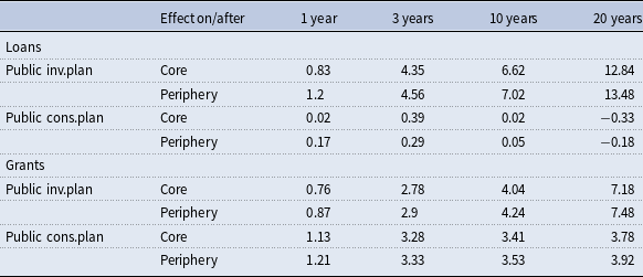
Main results are the following. First, a fiscal stimulus has a larger macroeconomic impact when it is financed by an EU grant, particularly after a shock on public consumption because the rise in taxes to fulfill the government budget constraint can be postponed. The intuition behind this result owes to the assumption that public investment is backed by public debt, while public consumption is usually backed by tax receipts, unless it is funded by EU grants.
Second, a European stimulus via NGEU is always more growth-enhancing than a national stimulus plan, with only one exception though. A national plan is more effective at boosting economic activity than a European plan funded by loans when it is led by the periphery thanks to a positive spillover effect: the increase in its risk premium leads to a higher wealth effect for households in the core, which then increases their consumption and thus the output.
Third, thanks to these wealth effects, fiscal multipliers are the highest after a shock on public investment when it is funded by EU loans, until 3 years after the shock. This effect is even strengthened when the economy is in a ZLB/post-Covid situation: the rise in the demand for loans accelerates the exit from the ZLB.
Overall, it also appears that NGEU grants play a more important role in financing public consumption than public investment, in sharp contrast with the actual operational architecture of NGEU. This is an important result that may contribute to explaining the limited appropriation of NGEU by EU Member States in cases where grants are attributed for public investment. In our setting, grants contribute to reducing the real costs of public consumption as they substitute with the rise in distortionary taxation.
As a side result, the systematic comparison between EU loans and grants funding offers a kind of natural experiment to calculate the opportunity cost of raising taxes in the economy. While the existence of this cost is trivial, evaluating its size is not: households who are not liquidity-constrained (Ricardian households) hold public debts and may benefit from a wealth effect. The latter disappears when spending is funded by grants, hence a trade-off for Ricardian households in their preference between loans and grants. By construction, EU loans increase public debt and activate the tax rule (taxes will increase to smooth the debt increase) whereas EU grants are simulated as a free lunch (they have no impact on public debt). In our simulations, the opportunity cost of taxes ranges between 0.2 and 0.9 percent of GDP per year.
We draw on two complementary strands of the literature: first, the literature on NGEU and, second, the literature on fiscal multipliers in DSGE models. To date, there are only a few contributions on multi-country macroeconomic impact of NGEU funds on the euro area.Footnote 3 Since NGEU disbursements will occur until the end of 2026, all studies revolve around ex-ante assessments using large macroeconomic models. Bańkowski et al. (Reference Bańkowski, Ferdinandusse, Hauptmeier, Jacquinot and Valenta2021), Codogno and Van Den Noord (Reference Codogno and Van Den Noord2022) and Pfeiffer et al. (Reference Pfeiffer, Varga and in ’t Veld2023) use respectively the EAGLE, NIGEM and the Commission’s QUEST DSGE models. Bańkowski (Reference Bańkowski2023) use also a smaller-scale semi-structural model (ECB Multi Country) to cross-check results. Shocks to public investment are calibrated on actual country spending allocations, hence the fiscal shock in Italy is higher than the shock in Germany. Except Codogno and Van Den Noord (Reference Codogno and Van Den Noord2022), the other two papers explicitly introduce the Leeper et al. (Reference Leeper, Walker and Yang2010) time-to-build specification for public investment and public capital. All papers compare EU loans and grants. They depart in only a few respects. First, Bańkowski et al. (Reference Bańkowski, Ferdinandusse, Hauptmeier, Jacquinot and Valenta2021) evaluate the impact on 5 large economies of the euro area whereas Codogno and Van Den Noord (Reference Codogno and Van Den Noord2022) and Pfeiffer et al. (Reference Pfeiffer, Varga and in ’t Veld2023) report estimates on all countries. Second, Bańkowski et al. (Reference Bańkowski, Ferdinandusse, Hauptmeier, Jacquinot and Valenta2021) assume that EU grants are repaid by an indirect tax levied uniformly for 30 years. Meanwhile, EU loans generate higher debt which is matched by a lump-sum tax. Pfeiffer et al. (Reference Pfeiffer, Varga and in ’t Veld2023) assume that debt repayments are also financed by lump-sum taxes, but EU loans are half-domestic funded. In contrast, we will disregard the repayment of grants, hence they appear as a free lunch for recipients.Footnote 4 Regarding loans repayments, we assume that they are matched by distortionary taxes on labor and private capital. In line with these three papers, we also explore the economic spillovers from NGEU fiscal stimulus. We present the outcomes of fiscal shocks on either the core or the periphery of the euro area when both have trade and financial interactions.
The paper also relates to the abundant literature on fiscal multipliers in DSGE models. Early contributions by Christiano et al. (Reference Christiano, Eichenbaum and Rebelo2011) and Woodford (Reference Woodford2011) highlighted that fiscal multipliers tend to be larger when nominal interest rates are at the ZLB, as monetary policy cannot offset fiscal expansions. Despite the ZLB, Corsetti et al. (Reference Corsetti, Kuester, Meier and Müller2013) show that sovereign risk may tend to reduce the output response to changes in government spending. This latter result has been refined recently drawing on liquidity spreads (Bayer et al. (Reference Bayer, Born and Luetticke2023), Bredemeier et al. (Reference Bredemeier, Juessen and Schabert2022)). Darracq-Pariès et al. (Reference Darracq-Pariès, Müller and Papadopoulou2023) introduce the interplay of corporate, bank and sovereign solvency risk and assess how it affects fiscal multipliers. Drautzburg and Uhlig (Reference Drautzburg and Uhlig2015) show that fiscal multipliers are sensitive to distortionary taxation. All these studies build on earlier work, such as Galí et al. (Reference Galí, López-Salido and Vallés2007) which demonstrated that fiscal policy’s efficacy is influenced by price stickiness and the extent to which households are credit-constrained.
The paper adds to the first strand of the literature with a systematic assessment of fiscal policies either EU-funded or domestically funded, and separating between public investment and public consumption. This allows to question the operational design of NGEU. In this respect, the paper highlights the real value added of NGEU vis-à-vis national fiscal plans and, thus, the possible benefits of a central fiscal capacity or a fiscal union. The paper adds to the second strand of the literature with the use of the extended approach to simulate a ZLB/post-Covid situation. In a morass like Covid-19 recession, the trade-off between a timely demand-oriented shock on public consumption and a long-lasting though gradual shock on public investment brings additional outcomes.
The remainder of the paper is organized as follows. Section 2 presents the theoretical setup. Section 3 and 4 present the calibration and moment matching. Section 5 presents the results of the simulations. Simulation results enable to quantify fiscal multipliers. They help to identify the conditions under which fiscal policy has most traction on economic growth in a monetary union. Finally, the extended path simulation enables to assess the impact of EU-funded stimuli under a ZLB situation after Covid-19 in section 6. Section 7 draws some policy implications while the last section concludes.
2. The model
We start with a simple model that we enrich with the necessary ingredients to represent the characteristics of various stimulus plans.
Our baseline model is an aggregated model of the euro area with public capital. It consists of four distinct agents: households, firms, a fiscal authority and a monetary authority. Households are divided into “unconstrained households” and “liquidity-constrained households,” differing in their access to financial markets. Unconstrained households are assumed to have access to financial markets, holding government-issued bonds. They also own firms, and profits from these firms are part of their income. In contrast, liquidity-constrained households do not have access to financial markets and are considered “hand-to-mouth.” All households both consume and supply labor. Regarding firms, we distinguish between producers of differentiated intermediate goods in monopolistic competition and producers of final goods. This methodology thus introduces some price rigidity. Producers of intermediate goods use labor and private and public capital as inputs. The fiscal authorities purchase the domestic good, invest in public capital, issue bonds to refinance their debt and raise taxes. A fiscal rule is assumed to guarantee the stability of public debt over a sufficient long horizon so that the debt-to-GDP ratio does not need to return to the target level at each period. As in Leeper et al. (Reference Leeper, Walker and Yang2010), we introduce the assumption that public investment takes the form of productive public capital, and that it is accumulated through a law of motion including some “time-to-build.” Finally, the monetary authority follows a Taylor-type interest-rate rule. This analytical framework corresponds to the closed-economy model, the results of which are presented in the appendix E.
The enriched model, summarized in Figure 1, substantially extends the baseline model with mainly two assumptions. First we consider two regions (or two countries) within the euro area, with international trade modeled through an extension of the NAWM model.Footnote 5 Second, we introduce country specific risk premia.
Two-region model with specific risk premia in a nutshell.

In the model presentation, we focus on the exposition of the core region, as the periphery is characterized symmetrically. Both regions/countries are part of a monetary union and share a single monetary authority. The first assumption implies that the model distinguishes between producers of differentiated intermediate goods in monopolistic competition and a set of two representative firms, which combine domestic and imported (tradable) intermediate goods into two distinct non-tradable final goods: private-consumption goods and private-investment goods. Producers of intermediate goods use labor, private and public capital as inputs (Leeper et al. Reference Leeper, Walker and Yang2010) producing domestic goods and exporting tradable goods. Considering trade between the two regions allows us to disaggregate the baseline model and to differentiate the effects on the core and the periphery. Additionally, this two-region model enables us to account for spillover effects, which are crucial to avoid underestimating the overall impact (unlike a simple aggregation of country-specific effects, see Pfeiffer et al. (Reference Pfeiffer, Varga and in ’t Veld2021)).
The second assumption involves the introduction of country-specific risk premia, resulting in the issuance of bonds at different interest rate levels. In particular, we introduce the idea that the core region and the periphery face a risk premium proportional to the deviation of the debt-to-GDP ratio from its equilibrium value: financial fragmentation can occur. The introduction of the risk premium is also important when we compare a European stimulus with a domestic one.
In our simulations, we use the augmented model of external trade alternately with and without risk premia to account for the assumption of a national vs. European stimulus plan.
The model can further be enriched when considering the possibility of a zero lower bound (ZLB). In that case, we impose a non-negativity constraint to the nominal interest rate, and we simulate the model through extended path tools. The model, in its simplicity, remains quite tractable and can provide clear insights on the impact of NGEU plans, allowing to clearly identify the interactions between core and peripheral countries in the euro area.
2.1. Households
2.1.1. Unconstrained households
Unconstrained households are denoted by
 $i$
and their utility function writes:
 \begin{equation} E_{t}\sum _{k=0}^{\infty }\beta ^{k}\left ( \epsilon _{t}^{z}\ln c_{i,t+k}- \frac {l_{i,t+k}^{1+\eta }}{1+\eta }\right ) \end{equation}
with
 $\beta ^{k}$
the discount factor of households and
 $\eta$
the inverse of Frish elasticity of work effort and
 $\epsilon _{t}^{z}$
is a preference shock that affects consumption and follows an AR(1) process detailed in section 2.6. The utility depends positively on individual consumption
 $c_{i,t}$
and negatively on labor supply
 $l_{i,t}$
.
Unconstrained households face the following budget constraint:
 \begin{eqnarray} &&\left ( 1+\tau _{t}^{c}\right ) c_{i,t}+b_{i,t}+I_{g,t}^{s}\nonumber \\[6pt] &=&\left ( 1-\tau _{t}^{W}\right ) w_{i,t}l_{i,t}+\psi _{t}^{g}\frac { R_{t-1}^{ea}}{\pi _{c,t}}b_{i,t-1} \end{eqnarray}
where
 $w_{i,t}$
is the real wage.
 $I_{g,t}^{s}$
is the investment in public capital stock.Footnote
6
 $\tau _{t}^{c},\tau _{t}^{W}$
are respectively taxes on consumption and wage and they are assumed to be exogenous and described in section 2.6.
 $b_{i,t}$
is the portfolio of sovereign bonds held by households.
 $\ R_{t}^{ea}$
is the risk free interest rate,
 $ \psi _{t}^{g}$
is the global risk premium attached to the households’ portfolio and
 $\psi _{t}^{g}\frac {R_{t-1}^{ea}}{P_{c,t}}$
can be interpreted as the global real return on portfolio of sovereign bonds.
When the recovery plan is European, such that each country borrows at the same rate, we assume that
 $\psi _{t}^{g}=1.$
When the recovery plan is national, we introduce a country-specific risk premium such that
 $\psi _{t}^{g}\neq 1$
, following the methodology outlined in Badarau et al. (Reference Badarau, Huart and Sangar2021).
In this specification, we assume that households hold a portfolio of sovereign securities composed of a proportion
 $b_{1}$
of domestic bonds (
 $ b_{i,t}^{d}$
) and
 $\left ( 1-b_{1}\right )$
of foreign bonds (
 $b_{i,t}^{\ast }$
).
 \begin{equation} b_{i,t}=\left ( b_{1}^{\frac {1}{\theta _{b}}}\left ( b_{i,t}^{d}\right ) ^{ \frac {\theta _{b}-1}{\theta _{b}}}+(1-b_{1})^{\frac {1}{\theta _{b}} }b_{i,t}^{\ast ^{\frac {\theta _{b}-1}{\theta _{b}}}}\right ) ^{^{\frac {\theta _{b}}{\theta _{b}-1}}} \end{equation}
 $\theta _{b}\gt 0$
is the constant elasticity of substitution between domestic and foreign bonds.
For the sake of simplicity, we assume that the linear combination of bond quantities leads to the same linear combination of risk. The global risk premium of the portfolio is therefore an aggregation of domestic (
 $\psi _{t}^{d}$
) and foreign risk premia (
 $\psi _{t}^{\ast }$
).Footnote
7
 \begin{equation} \psi _{t}^{g}=\left ( b_{1}\left ( \psi _{t}^{d}\right ) ^{1-\theta _{b}}+(1-b_{1})\left ( \psi _{t}^{\ast }\right ) ^{1-\theta _{b}}\right ) ^{ \frac {1}{1-\theta _{b}}} \end{equation}
The optimization problem of unconstrained households with respect to
 $ c_{i,t}$
,
 $b_{i,t}$
and
 $l_{i,t}$
gives the following first-order conditions:
 \begin{equation} \lambda _{i,t}=\frac {\epsilon _{t}^{z}}{c_{i,t}\left ( 1+\tau _{t}^{c}\right ) } \end{equation}
 \begin{equation} \lambda _{i,t}=\frac {\beta E_{t}\lambda _{i,t+1}\psi _{t}^{g}R_{t}^{ea}}{\pi _{c,t+1}} \end{equation}
 \begin{equation} w_{i,t}=\frac {l_{i,t}^{\eta }}{\lambda _{i,t}\left ( 1-\tau _{t}^{w}\right ) } \end{equation}
where
 $\lambda _{i,t}$
is the Lagrangian multiplier of unconstrained households optimization problem. Note that equation 6 represents the uncovered interest parity condition.
2.1.2. Liquidity constrained households
Liquidity constrained households are denoted by
 $j$
and their utility function writes:
 \begin{equation} E_{t}\sum _{k=0}^{\infty }\beta ^{k}\left ( \epsilon _{t}^{z}\ln c_{j,t+k}- \frac {l_{j,t+k}^{1+\eta }}{1+\eta }\right ) \end{equation}
The utility depends positively on individual consumption
 $c_{j,t}$
and negatively on labor supply
 $l_{j,t}$
. Liquidity constrained households face the following budget constraint:
 \begin{equation} \left ( 1+\tau _{t}^{c}\right ) c_{j,t}=\left ( 1-\tau _{t}^{W}\right ) w_{j,t}l_{j,t} \end{equation}
where
 $w_{j,t}$
is the real wage.
The solution of the optimization problem of these households with respect to
 $c_{j,t}$
and
 $l_{j,t}$
gives the following first order conditions
 \begin{equation} \lambda _{j,t}=\frac {\epsilon _{t}^{z}}{c_{j,t}\left ( 1+\tau _{t}^{c}\right ) } \end{equation}
 \begin{equation} w_{j,t}=\frac {l_{j,t}^{\eta }}{\lambda _{j,t}\left ( 1-\tau _{t}^{w}\right ) } \end{equation}
where
 $\lambda _{j,t}$
is the Lagrangian multiplier of liquidity constrained households optimization problem.
The presence of liquidity constrained households helps to capture Keynesian effects of fiscal policy as the economy is populated by agents for which the Ricardian equivalence does not hold. We anticipate that the effect of fiscal policy will be larger when the share of liquidity constrained households in the economy
 $\left ( 1-\mu \right )$
is itself larger.
2.2. Firms
2.2.1. Intermediate firms
Entrepreneurs produce intermediate goods under perfect competition regime. Each domestic intermediate goods firm produces goods
 $y_{t}$
that are sold domestically and abroad following a production function close to Leeper et al. (Reference Leeper, Walker and Yang2010):
 \begin{equation} y_{t}=T_{t}\left ( k_{t-1}^{\alpha }l_{f,t}^{1-\alpha }k_{g,t-1}^{\alpha _{g}}\right ) \end{equation}
where
 $k_{t-1}$
is productive capital rented by capital producer,
 $l_{f,t}$
is the aggregated labor demand such that
 $l_{f,t}=l_{i,t}^{\mu }l_{j,t}^{1-\mu }$
with
 $\mu$
the share of unconstrained households in the production function.
 $k_{g,t-1}$
is the aggregated public capital,
 $\alpha$
is the share of private capital in the production function and
 $\alpha _{g}$
is the elasticity of output with respect to public capital.
 $T_{t}$
is a permanent technology shock that follows an AR(1) process detailed in section 2.6.
Entrepreneurs denoted by
 $e$
, maximize their utility, which depends only on consumption, according to the following objective function
 \begin{equation} \mathbb{E}_{0}\sum _{k=0}^{\infty }\beta _{e}^{k}\ln \left ( {c_{e,t+k}} \right ), \end{equation}
where
 $c_{e,t}$
denotes entrepreneurs’ consumption, and
 $\beta _{e}$
the entrepreneurs’ discount factor. Entrepreneurs are assumed to discount the future more heavily than households such that their discount factor
 $\beta _{e}$
is lower than the households’ (
 $\beta _{e}\lt \beta$
).
Entrepreneurs’ decisions are taken according to the following budget constraint
 \begin{equation} c_{e,t}+w_{j,t}l_{j,t}+w_{i,t}l_{i,t}+R_{k,t}k_{t}=\frac {y_{t}}{x_{t}} +R_{k,t}\left ( 1-\delta _{k}\right ) k_{t-1}, \end{equation}
where
 $R_{k,t}$
is the nominal market price of capital and
 $x_{t}$
the markup of final over intermediate goods and
 $\delta _{k}$
is the depreciation rate of capital.
The optimality conditions of the entrepreneurs after maximization of their utility subject to their budget constraint and production function are:
 \begin{equation} \frac {1}{c_{e,t}}R_{k,t}=\beta _{e}\mathbb{E}_{t}\left [ \frac {1}{c_{e,t+1}} \left ( \alpha \frac {y_{t+1}}{x_{t+1}k_{t}}+R_{k,t+1}\left ( 1-\delta _{k}\right ) \right ) \right ] \end{equation}
 \begin{equation} w_{i,t}=\frac {\mu \left ( 1-\alpha \right ) }{l_{i,t}}\frac {y_{t}}{x_{t}}, \end{equation}
 \begin{equation} w_{j,t}=\frac {\left ( 1-\mu \right ) \left ( 1-\alpha \right ) }{l_{j,t}}\frac { y_{t}}{x_{t}}. \end{equation}
2.2.2. Capital good producer
Capital producers are in a competitive market. Their aim is to produce new capital and to sell it to entrepreneurs at the nominal market price
 $R_{k}$
.
Following Gerali et al. (Reference Gerali, Neri, Sessa and Signoretti2010), capital producers buy an amount
 $I_{t}$
of final good at the beginning of each period and the stock of old non-depreciated capital
 $\left ( 1-\delta _{k}\right ) k_{t-1}$
from entrepreneurs. Old capital can be converted one to one into new capital. We assume quadratic adjustment costs. Finally, the amount that capital good producers can produce is:
 \begin{equation} k_{t}=(1-\delta _{k})k_{t-1}+\left [ 1-\frac {\kappa _{k}}{2}\left ( \frac { \epsilon _{t}^{qk}i_{t}}{i_{t-1}}-1\right ) ^{2}\right ] I_{t} \end{equation}
where
 $I_{t}$
is the investment,
 $\kappa _{k}$
is the adjustment cost of a change in investment and
 $\epsilon _{t}^{qk}$
is a shock to the efficiency of investment, which follows an AR(1) process, detailed in section 2.6.
The profit maximization of the capital good producers delivers a dynamic equation for the real price of capital similar to Smets and Wouters (Reference Smets and Wouters2003, Reference Smets and Wouters2007):
 \begin{eqnarray} 1 &=&q_{k}\left ( 1-\frac {\kappa _{k}}{2}\left ( \frac {\epsilon _{t}^{qk}I_{t} }{I_{t-1}}-1\right ) ^{2}\right ) -\kappa _{k}\left ( \frac {\epsilon _{t}^{qk}I_{t}}{I_{t-1}}-1\right ) \left ( \frac {\epsilon _{t}^{qk}I_{t}}{ I_{t-1}}\right ) \notag \\[6pt] && +\, \beta _{e}\left ( \frac {c_{e,t+1}}{c_{e,t}}\right ) ^{-\sigma _{e,t}}R_{k,t+1}\kappa _{k}\left ( \frac {\epsilon _{t+1}^{qk}I_{t+1}}{I_{t}} -1\right ) \left ( \frac {\epsilon _{t+1}^{qk}I_{t+1}}{I_{t}}\right ) ^{2} \end{eqnarray}
2.2.3. Retailers
To motivate sticky prices, we assume implicit cost of adjusting nominal prices and monopolistic competition at retail level.
Retailers in a one-country model
A continuum of retailers of mass 1, indexed by
 $z$
buy intermediate goods
 $ y_{t}$
from entrepreneurs at a wholesale price
 $P_{t}^{w}$
, differentiate them at no cost and sell differentiated goods at a retail price
 $P_{t}$
.
Under this assumption,
 $x_{t}=P_{t}/P_{w,t}$
denotes the markup of final goods over that of intermediate goods.
Retailers
 $z$
bundle intermediate goods
 $y_{t}$
according to the following CES technology
 \begin{equation} y_{t}=\left [ \int _{0}^{1}y_{t}\left ( z\right ) ^{\frac {\epsilon _{t}-1}{ \epsilon _{t}}}dz\right ] ^{\frac {\epsilon _{t}}{\epsilon _{t}-1}}, \end{equation}
where
 $\epsilon _{t}$
is the elasticity of substitution between intermediate goods, detailed in Section 2.6.
Given the aggregate output index (Eq. 20), the price index is
 $P_{t}$
is
 \begin{equation} P_{t}=\left [ \int _{0}^{1}P_{t}\left ( z\right ) ^{1-\epsilon _{t}}dz\right ] ^{ \frac {1}{1-\epsilon _{t}}}, \end{equation}
such that each retailer faces an individual demand curve:
 \begin{equation} y_{t}\left ( z\right ) =\left ( \frac {P_{t}\left ( z\right ) }{P_{t}}\right ) ^{-\epsilon _{t}}y_{t}. \end{equation}
Retailers choose
 $P_{t}\left ( z\right )$
to maximize
 \begin{equation} \mathbb{E}_{t}\sum _{k=0}^{\infty }\Lambda _{t,k}\left [ P_{t}\left ( z\right ) y_{t}\left ( z\right ) -P_{t}^{w}y_{t}\left ( z\right ) -\frac {\kappa _{p}}{2} \left ( \frac {P_{t}\left ( z\right ) }{P_{t-1}\left ( z\right ) }-\pi _{t-1}^{\iota _{p}}\pi ^{1-\iota _{p}}\right ) ^{2}P_{t}y_{t}\right ], \end{equation}
where
 $\Lambda _{t,k}=\beta _{p}U_{c,t+k}/U_{c,t}$
denotes the stochastic discount factor, assuming the demand curve (Eq. 22) and wholesale price
 $P_{t}^{w}$
as given.
The optimality condition associated with the retailers’ problem is
 \begin{equation} \begin{array}{c} 1-\epsilon _{t}+\frac {\epsilon _{t}}{X_{t}}-\kappa _{p}\left ( \pi _{t}-\pi _{t-1}^{\iota _{p}}\pi ^{1-\iota _{p}}\right ) \pi _{t} \\[10pt] +\beta _{p}\left ( \frac {\epsilon _{z,t+1}}{\epsilon _{z,t}}\frac {c_{i,t}}{ c_{i,t+1}}\right ) \kappa _{p}\left ( \pi _{t+1}-\pi _{t}^{\iota _{p}}\pi ^{1-\iota _{p}}\right ) \pi _{t+1}\frac {y_{t+1}}{y_{t}}=0. \end{array} \end{equation}
In our model, a positive shock to
 $\epsilon _{t}$
leads to a decrease in the optimal value of markups, which can be interpreted as a negative price markup shock.
Retailers in a two-country model
A continuum of retailers of mass 1, indexed by
 $z$
buy intermediate goods
 $ y_{t}$
from entrepreneurs at a wholesale price
 $P_{t}^{w}$
, differentiate them at no cost and sell differentiated goods at a retail price
 $P_{h,t}(z),$
 $P_{x,t}(z),$
 $P_{im,t}(z)$
.
We assume that domestic and foreign retailers sell their differentiated good in both domestic and foreign markets with the same structure of price such that we get the same pricing equation with subscript
 $h$
,
 $x$
and
 $im$
for each differentiated goods (
 $h_{t}(z),$
 $EX_{t}(z),$
 $IM_{t}(z)$
)
The price setting behavior of intermediate good firm follows an adjustment à la Calvo implying that each period, a proportion
 $\left ( 1-\zeta _{h}\right )$
of firms receive permission to optimally reset their prices and choose
 $\widetilde {P}_{h,t}$
. Retailers that receive permission to reset prices choose
 $\widetilde {P}_{h,t}$
that solve the maximization problem taking as given
 $P_{t}^{w}$
and demand of differentiated good
 $ h_{t}(z),$
 $EX_{t}(z),$
 $IM_{t}(z)$
(demand is given in section 2.2.3)
The FOC obtained from the optimal pricing behavior is:
 \begin{equation} \sum _{k=0}^{\infty }\zeta _{h}E_{t}\left [ \Lambda _{t+k}\left ( \frac { \widetilde {P}_{h,t}}{P_{h,t+k}}-\frac {x}{x_{t+k}}\right ) h_{t+k}\left ( z\right ) \right ] =0 \end{equation}
where
 $x_{t}$
is the markup
 $\left ( P_{h,t}/P_{t}^{w}\right )$
which in steady state is equal to
 $x_{t}=\epsilon /(\epsilon -1)$
, with
 $\epsilon$
the elasticity of substitution between intermediate goods.
The aggregate price index
 $P_{h,t}$
evolves according to:
 \begin{equation} P_{h,t}^{1-\epsilon }=\left ( 1-\zeta _{h}\right ) \widetilde {P} _{h,t}^{1-\epsilon }+\zeta _{h}\left ( \pi _{h,t-1}\right ) ^{1-\epsilon } \end{equation}
Final good firms
Final good are obtained by aggregating intermediate goods through a CES aggregation tool:
 \begin{equation} h_{t}=\left ( \int \limits _{0}^{1}h_{t}\left ( z\right ) ^{\frac {\epsilon -1}{ \epsilon }}dz\right ) ^{\frac {\epsilon }{\epsilon -1}} \end{equation}
The demand equation of differentiated good are determined by choosing the optimal use of differentiated goods minimizing the expenditure for the bundles of differentiated goods subject to aggregation constraint:
 \begin{equation} h_{t}\left ( z\right ) =\left ( \frac {P_{h,t}(z)}{P_{h,t}}\right ) ^{-\epsilon }h_{t} \end{equation}
and aggregate price index are:
 \begin{equation} P_{h,t}=\left ( \int \limits _{0}^{1}P_{h,t}(z)^{1-\epsilon }dz\right ) ^{\frac {1 }{1-\epsilon }} \end{equation}
Final goods firms combine purchases of the domestically produced intermediate goods with the imported intermediate goods. They combine it into three distinct non-tradable goods, namely final consumption good
 $q_{c}$
, investment good
 $q_{i}$
and public consumption good
 $g$
. They are characterized symmetrically such that we use the same equation for all final goods, only modifying the subscript.
The representative firm produces non-tradable final private consumption good
 $q_{c,t}$
, combining the purchase of a bundle of domestically produced intermediate goods
 $h_{c,t}$
and a bundle of foreign imported goods
 $ im_{c,t}$
using a constant return to scale CES technology:
 \begin{equation} q_{c,t}=\left [ \nu _{c,t}^{\frac {1}{\mu _{c}}}\left ( h_{c,t}\right ) ^{1- \frac {1}{\mu _{c}}}+\left ( 1-\nu _{c,t}\right ) ^{\frac {1}{\mu _{c}}}\left ( im_{c,t}\right ) ^{1-\frac {1}{\mu _{c}}}\right ] ^{\frac {\mu _{c}}{\mu _{c}-1}} \end{equation}
where
 $\mu _{c}$
denotes the intratemporal elasticity of substitution between the bundles of domestic and foreign intermediate goods and
 $\nu _{c,t}$
measures the weight of domestic tradable intermediate goods.
The final goods firm chooses a combination of domestic
 $h_{c,t}$
and imported goods
 $im_{c,t}$
that minimizes expenditure
 $ P_{h,t}h_{c,t}+P_{im_{c},t}im_{c,t}$
, subject to technology constraint Eq. 30 and taking the input price indices
 $P_{h,t}$
and
 $ P_{im_{c},t}$
as given. Prices evolve according to:
 \begin{equation} P_{c,t}=\left [ \nu _{c,t}P_{h,t}^{1-\mu _{c}}+\left ( 1-\nu _{c,t}\right ) P_{im_{c},t}^{1-\mu _{c}}\right ] ^{\frac {1}{\mu _{c}-1}} \end{equation}
2.3. Monetary policy
As in Christoffel et al. (Reference Christoffel, Coenen and Warne2008), the common monetary authority sets the nominal interest rate according to the following log-linear Taylor rule:
 \begin{equation} R_{t}^{ea}=\phi _{R}R_{t-1}^{ea}+\left ( 1-\phi _{R}\right ) \left [ R^{ea}+\phi _{\pi }\left ( \pi _{c,t}^{ea}-\pi _{c}^{ea}\right ) +\phi _{gy}\left ( y_{gr,t}^{ea}-1\right ) \right ] +\epsilon _{R,t} \end{equation}
where
 $y_{gr,t}^{ea}=\frac {Y_{t}^{ea}}{Y_{t-1}^{ea}}$
denotes the euro area output growth,
 $P_{c,t}^{ea}$
is the euro area gross inflation rate and
 $\pi _{c}^{ea}$
is the euro area gross inflation at its steady state value,
 $\phi _{R}$
captures the degree of interest rate smoothing,
 $\phi _{\pi }$
and
 $ \phi _{gy}$
are policy coefficients reflecting the weights of inflation and the output gap, respectively and
 $\epsilon _{R,t}$
is an exogenous monetary policy shock identical for all European countries, following an AR(1) process detailed in section 2.6.
2.4. Government
Government expenditures are split between government consumption
 $g_{t}$
(supposed constant unless a shock occurs) and investment in public capital
 $ I_{g,t}$
. Government expenditures are financed by a set of fiscal instruments allowing to collect taxes on consumption and on labor income. Government expenditures are also financed by debt contracted with households
 $b_{i,t}$
. The government real budget constraint writes:
 \begin{equation} taxes_{t}+b_{i,t}=g_{t}+I_{g,t}+\frac {\psi _{t}R_{t-1}^{ea}}{\pi _{c,t}} b_{i,t-1} \end{equation}
where
 $taxes_{t}$
denotes the total tax revenues:
 \begin{equation} taxes_{t}=\tau _{t}^{C}c_{t}+\tau _{t}^{w}\left ( w_{i,t}l_{i,t}+w_{j,t}l_{j,t}\right ) \end{equation}
 $g_{t}$
is assumed to be exogenous such that:
 \begin{equation} g_{t}=g+\nu _{t}^{G} \end{equation}
with
 $\nu _{t}^{G}$
an exogenous shock of current expenditure described in section 2.6.
The borrowing rate associated with the issuance of sovereign debt is elastic to the level of current debt. Thus, the risk premium depends on the deviation of the debt-to-GDP ratio from its target:
 \begin{equation} \psi _{t}=\exp \left ( \psi _{n}\left ( b_{i,t-1}-\overline {b}p_{y}y\right ) \right ) \end{equation}
where
 $\psi _{n}$
is the sensitivity coefficient of the risk premium to public indebtedness and
 $\overline {b}$
is the steady-state target for the stock of real debt in proportion to GDP (Badarau et al. Reference Badarau, Huart and Sangar2021).
2.4.1. Fiscal policy
We assume that the government fulfills a fiscal rule that forces the primary structural balance to adjust in order to stabilize the long run debt-to-GDP ratio. The government’s primary structural balance (
 $S_{Struct}$
) is defined as:
 \begin{equation} Sstruc_{t}=\tau _{t}^{C}c+\tau _{t}^{w}\left ( w_{i}l_{i}+w_{j}l_{j}\right ) -g-I_{g} \end{equation}
where variables without time subscript relate to their steady state values. Shifts to public investment and public consumption are interpreted as structural shocks to public finances. Meanwhile, we assume, following LeMoigne et al. (Reference LeMoigne, Saraceno and Villemot2016), that the government is tied to the following golden rule of public finance:
 \begin{equation} Sstruc_{t}-\left ( \left ( \frac {\psi _{t}R_{t-1}^{ea}}{\pi _{c,t}}-1\right ) b_{i,t-1}\right ) =\phi _{b}\left ( b_{i,t-1}-\overline {b}p_{y}y\right ) -\epsilon _{t}^{G} \end{equation}
where
 $\phi _{b}$
is the sensitivity of lump-sum taxes to debt-to-output ratio and
 $\epsilon _{t}^{G}$
is an exogenous shock allowing for a temporary deviation from the fiscal rule.
2.4.2. Public investment
In order to align with the principles of NGEU, the European economic recovery plan centered around investment, our model must incorporate public investment. To achieve this, we adopt the framework introduced by Leeper et al. (Reference Leeper, Walker and Yang2010), which involves categorizing public expenditures into two distinct components: consumption and investment in public capital (
 $I_{g,t}$
).
Additionally, and still following Leeper et al. (Reference Leeper, Walker and Yang2010),
 $I_{g,t}$
stands for the implemented government investment which is different from authorized government investment
 $A_{t}.$
Leeper et al. (Reference Leeper, Walker and Yang2010) assume that government investment turns into public capital through a time-to-build process, such that the authorized government spending is not immediately implemented and productive.
The law of motion for public capital is:
 \begin{equation} k_{g,t}=(1-\delta _{g})k_{g,t-1}+A_{t-N} \end{equation}
where
 $N$
is the number of quarters between granting budget authority and completing a project,
 $\delta _{g}$
the depreciation rate of public capital, and
 $A_{t-N}$
the authorized government investment (the stock). The law of motion entails that public capital accumulates on a much longer scale of time (n) than private capital because the stock of public capital is useful only once the project is fully completed.
We add another hypothesis of Leeper et al. (Reference Leeper, Walker and Yang2010): spending outlays authorized by the government occur over several periods. Thus, we consider the spending rates
 $\{\phi _{0},\phi _{1},\ldots, \phi _{N-1}\}$
from the date the investment is authorized (
 $t=0$
) to the period before project completion (
 $t=N-1$
). Thus we have:
 \begin{equation} I_{g,t+1}=\sum _{n=0}^{N-1}\phi _{n}A_{t-n} \end{equation}
with
 $A_{t}$
decided by the government at each period, which follows an AR(1) process described in section 2.6.
Moreover, following LeMoigne et al. (Reference LeMoigne, Saraceno and Villemot2016), we take into account the possibility that private investment will crowd-in the projects. In order to model this, we force part of the Ricardian (unconstrained) agents’ savings into public capital stock in the form of a lump-sum tax (
 $I_{g,t}^{s}$
):
 \begin{equation} (1-\mu )I_{g,t}^{s}=Lp\times \left ( I_{t}^{S}-I^{S\ast }\right ) \end{equation}
with
 $Lp$
the amount of the private leverage effect.
This lump-sum tax is taken directly from the Ricardian agents’ savings, thus enter their budget constraint (Eq. 2) as well as the goods’ market clearing condition. It is directed into the public capital stock:
 \begin{equation} k_{g,t}=(1-\delta _{g})k_{g,t-1}+A_{t-(N-1)}+Lp\times \left ( A_{t-(N-1)}-A^{\ast }\right ) \end{equation}
2.5. Equilibrium and market clearing
Market clearing conditions write:
 \begin{equation} y_{t}=c_{,t}+I_{t}+g_{t}+I_{g,t}+I_{g,t}^{s}+\frac {1-s}{s}EX_{t}-IM_{t} \end{equation}
 \begin{equation} q_{c,t}=c_{t} \end{equation}
 \begin{equation} q_{i,t}=I_{t} \end{equation}
Aggregation equations are
 \begin{equation} w_{t}=\left ( 1-\mu \right ) w_{j,t}+\mu w_{i,t} \end{equation}
 \begin{equation} c_{t}=\left ( 1-\mu \right ) c_{j,t}+\mu c_{i,t}+c_{e,t} \end{equation}
 \begin{equation} h_{t}=h_{c,t}+h_{i,t}+g_{t}+I_{g,t}+I_{g,t}^{s} \end{equation}
 \begin{equation} im_{t}=im_{c,t}+im_{i,t} \end{equation}
2.6. Stochastic structure
The structural shocks are assumed to follow a first-order autoregressive functional form:
 \begin{equation} X_{t}=\left ( 1-\rho _{X}\right ) \overline {X}+\rho _{X}X_{t-1}+\eta _{t}^{X}, \end{equation}
where
 $X_{t}\in \left \{ \epsilon _{t}^{z},T_{t},\tau _{t}^{c},\tau _{t}^{W},\epsilon _{t}^{G},A_{t},\nu _{t}^{G}\right \}$
,
 $\overline {X}$
is the steady-state value of
 $X_{t}$
,
 $\rho _{X}\in \left [ 0,1\right [$
is the first-order autoregressive parameter of the shock
 $X_{t}$
and the innovation
 $\eta _{t}^{X}$
is an
 $i.i.d$
normal error term with zero mean and standard deviation
 $\sigma _{X}$
.
3. Calibration
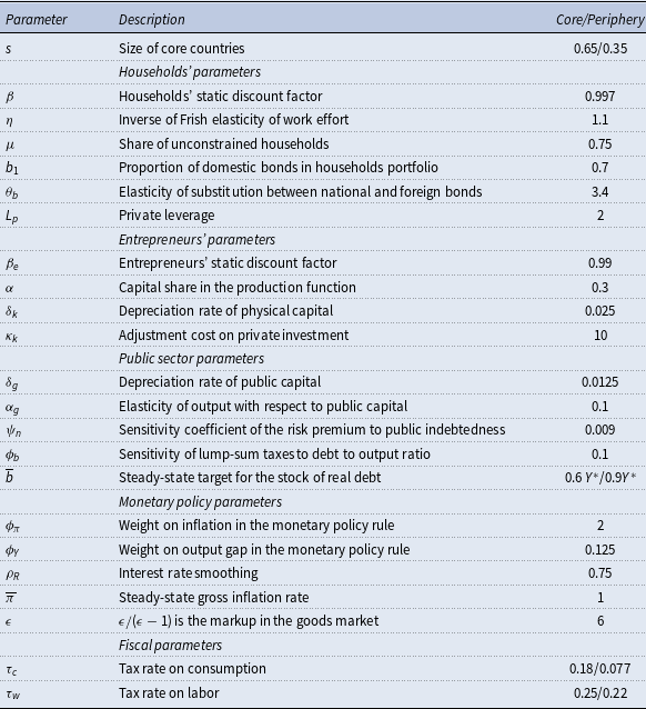
The model is set at quarterly frequency. Parameters are calibrated according to the literature and to historical steady-state ratios. The list of parameters is reported in Table 1.
Definition of models’ parameters

We assume that peripheral countries represent a lower economic weight than core countries. We set the relative size of the core countries to
 $s=0.65$
. The discount factor of households
 $\beta$
is calibrated to
 $0.997$
allowing the nominal rate to be close to
 $2$
percent. The inverse of Frish elasticity of work effort
 $\eta$
is calibrated to
 $1.1$
in line with the value in Galí (Reference Galí2008). Labor income share of unconstrained households
 $\mu$
is
 $ 0.75$
such that
 $25\%$
of households are assumed to be non-Ricardian.Footnote
8
Entrepreneurs are assumed to discount the future less heavily than households such that
 $\beta _{e}\lt \beta$
. We calibrate
 $\beta _{e}$
to
 $0.99$
. The capital share in the production function
 $\alpha$
is set at
 $0.25$
. Depreciation rate of physical capital
 $\delta _{k}$
is
 $0.025$
corresponding to a
 $10$
percent depreciation rate per year. The adjustment cost on private investment
 $\kappa _{k}$
is
 $10$
, in line with the value estimated by Gerali et al. (Reference Gerali, Neri, Sessa and Signoretti2010). Following LeMoigne et al. (Reference LeMoigne, Saraceno and Villemot2016), we calibrate the depreciation rate of public capital
 $\delta _{g}$
to
 $ 0.0125$
. The elasticity of output with respect to public capital
 $\alpha _{g}$
is calibrated to
 $0.1$
and the private leverage
 $L_{p}$
to
 $2.$
We assume that core and peripheral countries do not share similar steady-state values of the debt-to-GDP ratio. Core countries have a value of 60 percent of GDP (
 $\overline {b}=0.6Y^{\ast }$
) while peripheral countries have a ratio of 90 percent of GDP (
 $\overline {b}=0.9Y^{\ast }$
). This assumption thus introduces a deviation from the fiscal rules embedded in the Stability and Growth Pact until 2020: it involves that debt targets are country-specific as advocated by Martin et al. (Reference Martin, Pisani-Ferry and Ragot2021).Footnote
9
The monetary parameters are standard. On the fiscal side, we set the steady state value of the tax rate on consumption purchases
 $\tau _{c}$
and labor income
 $\tau _{w}$
for core and periphery to
 $0.183$
and
 $0.077$
and to
 $0.25$
and
 $0.22$
respectively.
Following Badarau et al. (Reference Badarau, Huart and Sangar2021), we set the home bias in sovereign bond holding (
 $b_{1}$
) to
 $0.7$
, reflecting a strong preference for domestic government debt. Similarly, we calibrate the sensitivity of the risk premium to public indebtness (
 $\psi _{n}$
) at
 $0.009$
. Finally, the elasticity of substitution between national and foreign bonds (
 $\theta _{b}$
) is set to
 $3.4.$
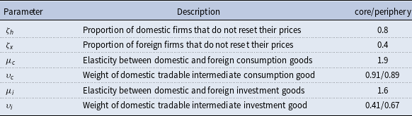
International trade parameters are given in Table 2 and are taken from the value estimated by the NAWM model. Regarding final-good production, the home bias parameters
 $\upsilon _{c}$
and
 $ \upsilon _{i}$
are calibrated so that the model replicates the import content of consumption and investment spending stemming from the input-output tables for the euro area.
Commercial trade parameters

4. Moment matching
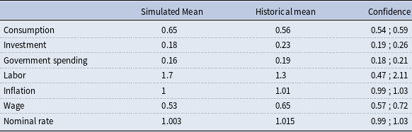
In accordance with the balanced-growth assumption, we calibrate the parameters such that key steady-state ratios generated by the model match their empirical counterparts over the sample period.
To conduct our moment matching, we use the area-wide model database. To compare the data simulated by the model with the observed variables, we make some transformations to the database, which are detailed in the Appendix D.
Table 3 presents the first order moment (mean) obtained from the aggregated model of the euro area. The simulated moment of the model align pretty well with historical data of the euro area.Footnote 10
Moment matching—First order

Notes: Historical moments (Hist.) are calculated using data from 1970 to 2018. The averages represent the corresponding variable’s steady-state ratio to the output. A 5% confidence interval is used across the 190 observations for each time series assuming a normal distribution.
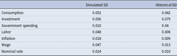
Table 4 presents the simulated standard deviation (SD) based on calibration presented in section 3. Our model successfully captures key second order moments. However, second moments for labor and wage are not well replicated, primarily due to the simplified labor market modeling (e.g., wage rigidities are ignored).
Moment matching—Second order

Notes: Historical moments (Hist.) are calculated using data from 1970 to 2018.
5. Assessing different features of fiscal stimulus
In order to carry out our analysis, we consider two alternative scenarios in which a shock occurs either on public consumption, or on productive public investment. These two scenarios allow us not only to distinguish the different spending possibilities offered to the EU Member States but also to study the incidence of their funding via either loans or grants.
In contrast with a shock on public consumption, the public investment shock includes a time-to-build of 12 periods (3 years) and a private leverage of 2. In both cases, we assume a public spending shock of 1 percent of GDP,Footnote 11 knowing that the NGEU shock should amount to 5 percent of the euro area’s GDP, i.e., 5 times larger than the simulated shock. Scaling the shock to 1 percent of GDP and not to the maximum amount of grants and loans attributed to the different Member States permits to abstract from the conditionality attached to NGEU funding or the potential absorption capacity constraints faced by Member States.Footnote 12
All simulations are performed alternately for the core and the periphery. Incorporating a two-country model with spillover (trade and financial) effects prevents the underestimation of shocks that would be associated with an ex post aggregation of country-specific models (see Pfeiffer et al. Reference Pfeiffer, Varga and in ’t Veld2021)Footnote 13 .
We differentiate between three structural frameworks. Firstly, the stimulus plan is national, meaning there is no European sovereign bond market. Each country issues its own bonds with specific risk premia, which are elastic to the current debt level. Secondly, countries share a common risk premium. This corresponds to a situation where the EU borrows at a risk-free rate and transfers the benefits to the member states, simulating the loans-related part of NGEU. Finally, we introduce the grant-related part of NGEU after neutralizing the impact of an increase in public spending on the budget constraints of the two countries.Footnote 14
5.1. Public consumption shock
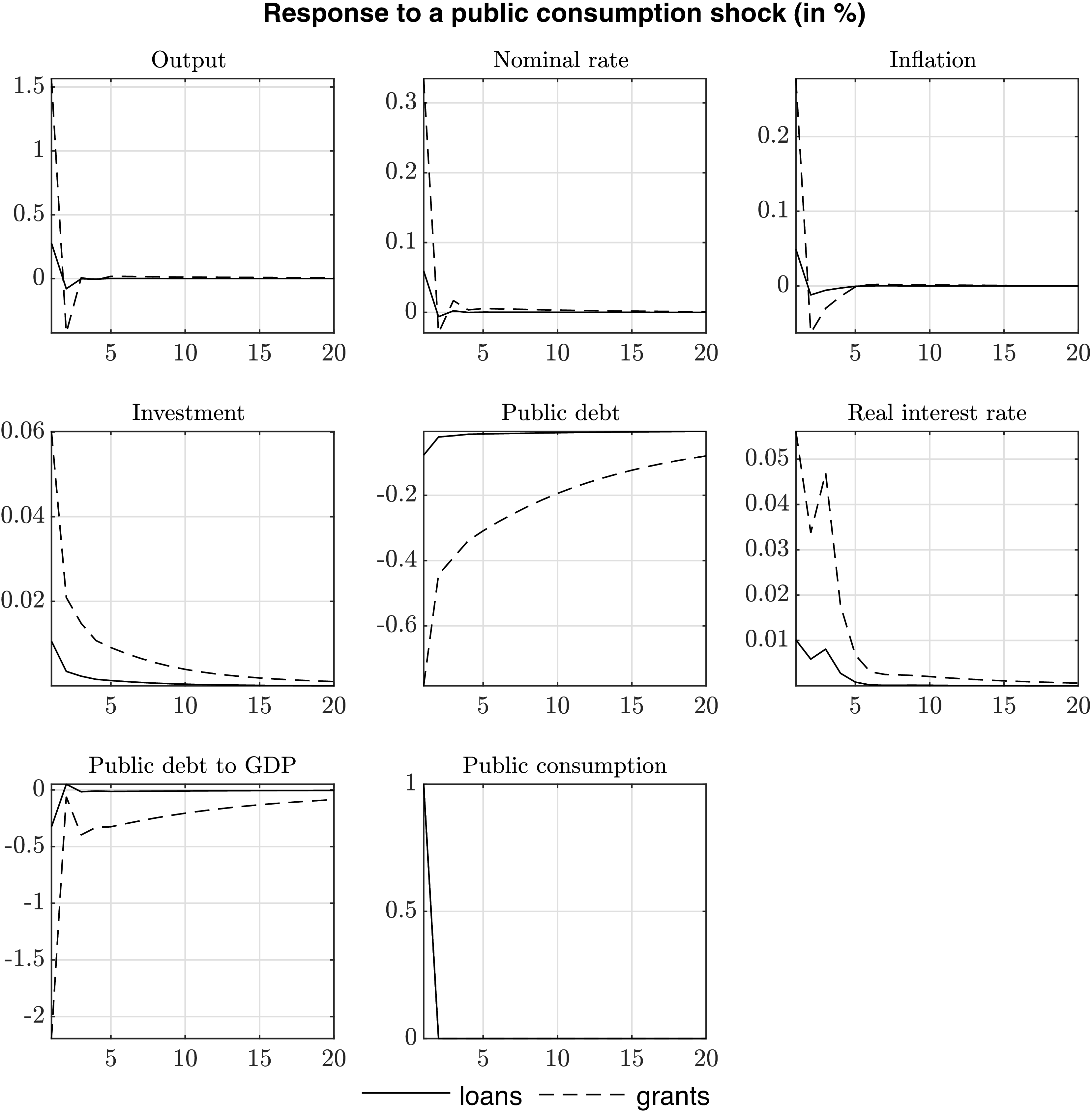
Whether the initial shock arises in the core (Figure 2) or the periphery (Figure 3), the rise in public consumption leads to an increase in output relative to its long-term equilibrium level. However, the effect on output is not persistent. Comparing the different funding frameworks shows that a recovery financed by grants (dotted line) has a larger effect on production than one financed by EU loans (dashed line) or national funding (solid line) in the country hit by the shock. Actually, EU or national loans require an increase in distortionary taxation which is absent if funding stems from a grant.
Public consumption shock in the core—model with national stimulus, EU loans or grants.

Public consumption shock in the periphery—model with national stimulus, EU loans or grants.

The growth effect after a fiscal stimulus funded with an EU grant increases tax receipts and leads to a reduction in public debt. According to the fiscal rule (Eq. 38), tax rates can decline and generate a crowding-in effect between public consumption and private investment in the country hit by the shock, despite rising policy rate. Conversely, the country which is not directly hit by the shock sees a reduction of private investment because of the rise in the policy rate following the shock in the neighbor country.
The comparison of the origin of the shock (Figure 2 vs. 3) reveals that the short-term growth impact of a public consumption shock is twice higher when it occurs in the core than in the periphery. A shock in the core shows an initial positive effect on the periphery that rapidly disappears. In contrast, a shock in the periphery immediately weighs on the core. With funding via grants, the lower public debt in the periphery limits the wealth effect in the core.
5.2. Public investment shock
The macroeconomic effects after a public investment shock (either in the core, see Figure 4, or in the periphery, see Figure 5) are similar to those detailed in the closed-economy framework of LeMoigne et al. (Reference LeMoigne, Saraceno and Villemot2016). By construction and in contrast with the shock on public consumption, the investment stimulus plan has persistent effects. The simulation of the public investment shock shows two phases. The first one corresponds to the time-to-build period of public capital. During this phase, public investment leads to an increase of aggregate demand, up to respectively
 $0.6\%$
(shock on the core) and
 $0.2\%$
(shock on the periphery) above the long-run equilibrium level, and to an increase of inflation. It triggers a reaction of monetary policy that hikes the nominal interest rate. This in turn dampens the expansionary effect of the initial shock. These effects explain the U-shaped GDP reaction function between quarters 1 and 12 following the shock. In the second phase of the shock, the investment effect disappears (explaining the sharp drop at
 $t=12$
, when GDP shortly becomes negative); however, the new infrastructures become productive, leading to a positive supply effect. Production remains for a very long time above its steady state value, by
 $0.2\%$
(regardless of the origin of the shock) as long as the new public capital is not completely depreciated. The increase in aggregate supply also leads to lower inflation, and therefore to a softened monetary policy.
Public investment shock in the core—model with national stimulus, EU loans or grants.

Public investment shock in the periphery—model with national stimulus, EU loans or grants.

In contrast with a shock on public consumption, the funding of a shock on public investment does not matter much, at least in the first phase. Actually, the dynamic responses of the output are very similar. The main difference lies in the evolution of public debt: by construction, it increases under the EU common loan framework whereas it declines under the grant framework. Overall, these results highlight how intricate the wealth effect might be with distortionary taxation. Under the loans framework, the rise of public debt which paves the way for the wealth effect is limited by the rise in distortionary taxation. The results also show that a national stimulus package will have smaller effects than a European stimulus package funded via NGEU. Since public investment is financed by new issuances of national public debt, risk premia increase and crowd-out private consumption and investment.
Whether implemented by the core or by the periphery, the investment stimulus plan has a positive overall effect on aggregate GDP. However, thanks to trade spillover effects, a recovery through investment in the periphery has beneficial effects in the short term in the core. Peripheral countries, on the other hand, have to wait longer to see the beneficial effects of an investment stimulus in the core, but then benefit from higher spillovers. This owes to the (realistic) assumption that the degree of openness of the core is smaller than that of the periphery.
5.3. The multiplier effects of the stimulus
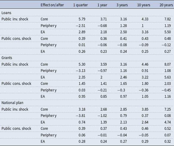
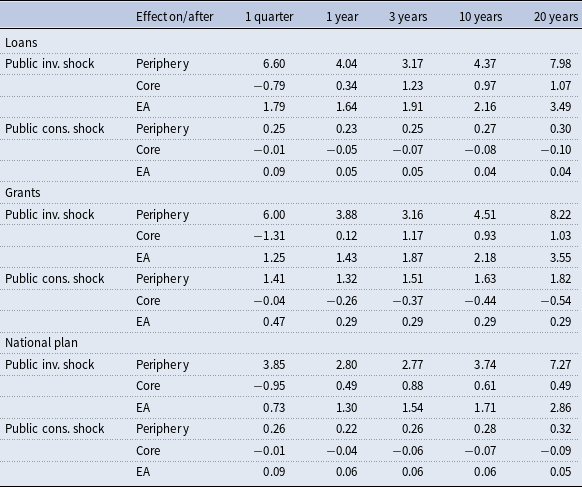
The former sub-sections have highlighted the macroeconomic mechanisms triggered by the fiscal shocks. Now, a numerical analysis of fiscal multipliers helps to discriminate between the different features of a fiscal stimulus. The (undiscounted) cumulated multipliers of additional GDP after the different stimulus packages are reported in Tables 5 and 6 for both countries (core and periphery). Table 5 (resp. 6) reports a shock originating in the core (resp. the periphery). Hence, we not only report a proxy for the effectiveness of the fiscal shock on the country where the shock occurred but also the spillovers on the output of the other country.
Fiscal multipliers by type of stimulus and by type of funding—Shock on the core

Fiscal multipliers by type of stimulus and by type of funding—Shock on the periphery

While the multiplier effects might seem very large, they are not unusual in the literature. On impact, the cumulative multiplier effects are consistent with those of Pappa and Canova (Reference Pappa and Canova2021) after an investment shock funded via the European Regional Development Fund. After one year, they are close to those found by Bouakez et al. (Reference Bouakez, Guillard and Roulleau-Pasdeloup2017) in the US following the American Recovery and Reinvestment Act of 2009. In the longer run, Ramey (Reference Ramey2020) shows multiplier effects close to 9 or even 10 in the literature using New-Keynesian models. Pfeiffer et al. (Reference Pfeiffer, Varga and in ’t Veld2023) find lower multiplier effects than those reported in the table below because they include a third region to the model, the rest of the world. Hence, they report higher import leakages from a European fiscal stimulus than we do.
Reporting undiscounted fiscal multipliers has a possible important advantage in terms of the political economy of reforms. The use of a discount factor is plagued with uncertainty, a point well known and for long in the literature about investments with delayed effects in the area of climate policy (see, e.g., Newell and Pizer Reference Newell and Pizer2004). Unless the discount factor increases with the investment horizon (see, e.g., Gollier Reference Gollier2002), the use of a constant discount factor may act as a drag on (public) investment and may give incentive to prefer public consumption with more immediate effects.
From Tables 5 and 6, there are 6 main outcomes which hold similarly for both countries (core and periphery).
First, public investment shocks have a more substantial impact on GDP than public consumption shock. It appears so on impact, one year after the shock, and in the longer run when the time-to-build process has boosted the productive capacities of the different economies. This highlights the mixture of demand-driven and supply-driven features of public investment in contrast with public consumption and also the cost of distortionary taxation arising from a fiscal impetus on public consumption.
Second, after a shock on public investment, the impact on GDP is the highest for the country where the shock occurred if it is funded by EU loans until the "time-to-build” has occurred. After that, beyond 3 years, the impact on GDP is the highest when the fiscal impetus is funded by grants. During the first 3 years after the shock, the wealth effect from Ricardian consumers positively contributes to GDP.
Third, maximum spillovers from the fiscal impetus are achieved 3 years after the shock and when it is funded by EU loans. This confirms that wealth effects matter: EU loans, but not grants, lead to a rise in public debts that in turn generates some wealth effects for Ricardian households.
Fourth, the simulations give an appraisal of the real advantage of grants vs. loans. Actually, grants permit to escape a rise in taxes to fund the increase in public consumption and limit that of public debt. The opportunity costs of raising taxes after a shock to public consumption can be proxied by the difference between the multiplier effects when the shock is funded via grants or loans. For the aggregate area, it amounts to + 0.7 percentage points of GDP after 1 quarter if the shock has hit the core, and to + 0.4 pp if it has hit the periphery. It will climb to + 0.9 pp after 20 years in the first case, but decrease to + 0.25 pp in the second case.
Fifth, public investment multipliers also show that the NGEU program would give GDP more traction in both the short and long run compared to a similar fiscal shock financed by domestic debt. This is due to the effect of risk premia that adjust as a result of the increase in public debt. Despite the wealth effect, the rise in the risk premia and in debt after a domestic shock produces a decline in private investment that weighs on aggregate demand. The superiority of a European investment shock on a domestic investment shock shows only one exception: after 1 year, a shock on the periphery has a higher GDP spillover on the core if the shock has been a domestic one. This owes to the higher rise of peripheral debt that generates a higher wealth effect in the core, in contrast to a European-funded shock in the periphery. This effect is limited in time, though.
Sixth, NGEU grants are more important for public consumption than for public investment. Comparing cumulative fiscal multipliers after a shock on public consumption shows that they are much higher when spending is funded by grants rather than loans: while the short-term positive demand effect of the shock funded by a grant gives rise to a sharp increase in the nominal interest rate, the lower debt overturns the latter (the risk premium declines) which transmits into a lower real interest rate and a rise in private investment. In contrast, the rise in distortionary taxes when EU loans are used dampens the impact on output. The choice between loans and grants after a public investment shock appears less crucial (cumulative fiscal multipliers are very close): the mechanism of the golden rule of public finance which prevails when public investment increases prevents the rise in distortionary taxation that follows a rise in public consumption. The respective impacts on GDP of the wealth effect and higher taxation will somewhat neutralize: public debt and the wealth effect will be a bit higher under EU loans financing than under grants; meanwhile, higher taxation will also be a bit higher. All in all, whatever the EU financing instrument, a shock on public investment will produce almost the same monetary reaction. In contrast to a shock on public consumption, the rise in the nominal interest rate is gradual.
5.4. Sensitivity analysis
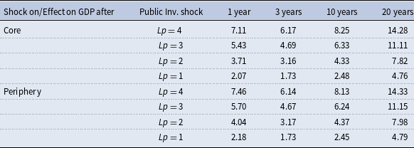
Results remain consistent across a range of plausible values for parameters. For instance, robustness analyses show that the values of the public investment multiplier are sensitive to the level of leverage, set at 2 in the benchmark case (see Table 7). This level could well be lower or higher, making the cumulative multiplier effects discussed so far either over- or under-estimated.
Fiscal multipliers of public investment financed by loans, by level of leverage

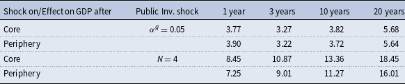
Moreover, fiscal multipliers are sensitive to the assumption about how productive public capital may be. A lower capital productivity reduces the fiscal multiplier of public investment in the long run (Table 8). Symmetrically, a lower time-to-build period of public investment increases the fiscal multiplier.
Fiscal multipliers of public investment financed by loans, for alternative calibrations

6. The NGEU under a zero lower bound: a post-Covid illustration
This section simulates the same fiscal shocks as in the previous section but now under the economic conditions that prevailed after the Covid 19 crisis. In particular, we study the effects of a fiscal stimulus when the economy has already been submitted to a series of shocks that deteriorate output and put the policy rate at the zero-lower-bound (ZLB). We introduce a non-linear Taylor rule which removes occurrences of a negative nominal interest rate:
 \begin{equation} R_{t}^{ea}=\max \left(\phi _{R}R_{t-1}^{ea}+\left ( 1-\phi _{R}\right ) \left [ R^{ea}+\phi _{\pi }\left ( \pi _{c,t}^{ea}-\pi _{c}^{ea}\right ) +\phi _{gy}\left ( y_{gr,t}^{ea}-1\right ) \right ] +\epsilon _{R,t};1 \right) \end{equation}
We model the post-Covid situation by applying symmetric negative shocks to the core and the periphery. Negative shocks imply a sharp drop in the rate of time preference. This amounts to lowering the real interest rate of the economy.
We solve the model using the extended path method. This method takes account of non-linearities and permits a reasonable treatment of expectations. The agents are surprised by the shocks at all periods. Extended path simulations also allow us to calibrate the size of the shocks as close as possible to the post-Covid situation.
6.1. Fiscal stimulus, ZLB and loans
We analyze the path of nominal interest rate (Figure 6) and GDP (resp. Figure 7 on core and Figure 8 on periphery) when the economy is plunged into a post-Covid situation under three scenarios. In the first scenario (dotted line), there are no fiscal plans (or no fiscal reactions to the shocks). The second scenario (dashed line) implies a public investment recovery plan while the third scenario (solid line) is a public consumption recovery plan. In these simulations, all shocks are assumed to affect the core and the periphery in the same proportion and fiscal plans are financed by loans.Footnote 15
Impact on interest rates of a fiscal shock in the context of a ZLB—Financing by loans.

The stimulus package, whether it is an increase in consumption or investment, leads to an increase in aggregate demand which contributes to increasing inflation and therefore triggers an intervention from monetary authorities via rising policy rates. The investment-led recovery allows for a larger and more long-lasting exit from the ZLB than a consumption-led policy since the latter also generates a rise in distortionary taxation.
Impact on core GDP of a fiscal shock in the context of a ZLB—Financing by loans.

Whatever the nature of the EU recovery plan (public investment- or consumption-related), its implementation closes the output gap fairly quickly. However, at the end of the time-to-build period, or once public consumption spending is completed, GDP falls significantly. In the long run, GDP remains below its steady state if the recovery is carried out by public consumption. On the other hand, it is durably above its steady state with a recovery carried out by an investment stimulus. This latter outcome is consistent with Bouakez et al. (Reference Bouakez, Guillard and Roulleau-Pasdeloup2020).
Impact on periphery GDP of a fiscal shock in the context of a ZLB—Financing by loans.

6.2. Fiscal stimulus, ZLB and grants
We run the same simulations as in the former subsection but we analyze the path of nominal interest rate (Figure 9) and GDP (resp. Figure 10 on core and Figure 11 on periphery) focusing on grants. The real impacts on the core and the periphery share similar shapes as those reported when the fiscal shock was funded by loans. However, a public consumption shock financed by a grant now shows a larger impact on GDP in the short run than a shock on public investment. It also shows a larger impact than the same shock funded by loans. The strong and immediate impact of public consumption coupled with the free-lunch opportunity offered by a grant triggers a sharper rise in the policy rate. The debt-economy provided by grants thus limits recourse to taxes while the ZLB is more rapidly overcome. This illustrates again the opportunity costs of loans vs. grants. In the longer run, a shock on public investment funded by grants has a higher impact on GDP, in comparison with a shock on public consumption: this highlights the supply-driven property of public investment in the long run.
Impact on interest rates of a fiscal shock in the context of a ZLB—Financing by grants.

Impact on core GDP of a fiscal shock in the context of a ZLB—Financing by grants.

6.3. Fiscal stimulus, the EU and the ZLB: a summary of results
Table 9 summarizes the main outcomes of the simulations of policy shocks under an extended-path approach. For each type of fiscal shock (on public investment or on public consumption) and each type of funding (loans or grants), Table 9 shows the extra-gain of the policy, including cross-spillovers, vis-à-vis no policy at all. In most cases, an EU-wide fiscal reaction to the Covid-like crisis brings positive and large output effects. Exception to this occurs when the core and peripheral countries target public consumption expenditures and fund fiscal policy via loans. The early rise in the nominal interest rate coupled with raising taxes slows down the pace of the recovery: the output effect peaks at + 0.3–0.4 pp after 3 years and turns negative in the very long run. In contrast, grants are shown to be superior to loans after the Covid-like crisis when they fund a shock on public consumption. In this case, output effects are larger than with EU loans. This result is consistent with those reported with stochastic simulations and a linear Taylor-type rule for monetary policy.
Cumulative effect on output of a European fiscal stimulus, in comparison with no fiscal stimulus, in percentage points of GDP

Impact on periphery GDP of a fiscal shock in the context of a ZLB—Financing by grants.

There is a new result when the extended path approach is used and a ZLB/Covid-like situation is simulated. Now grants are surpassed by loans to fund public investment: whatever the horizon, the cumulative fiscal multipliers after a shock on public investment are always larger when they are backed by loans. In this situation, the wealth effect brings some additional traction on economic activity.
7. Policy implications
The model outcomes highlight a few features with some policy implications. First, the simulations show a trade-off between a fast recovery and a resilient economy which mirrors the double objective of NGEU and its so-called Recovery and Resilience Facility. While public consumption permits to accelerate the economic recovery, public investment favors the resilience of the economy. By choosing to focus on public investment, the EU has given preference towards resilience or towards the long run. While it may not be a problem in itself, it has certainly blurred the communication of the EU on the merits of NGEU. Actually, and although the NGEU fiscal program has been effective at boosting economic activity after the pandemic, the results of the simulations show that the recovery would have been even faster had the fiscal stimulus been targeted towards public consumption or had loans been backing the fiscal stimulus on public investment. Unfortunately, these two options were not included in the operational design of NGEU.
Second, a larger share of grants has been requested by EU Member States so far than their share of loans. However, the simulations show that using one or another does not make a large difference when public investment is concerned. Unless the allocation of NGEU funds is changed, from public investment to public consumption, the reluctance of requesting EU loans is suboptimal: fiscal multipliers after a shock on public investment are almost as high under EU loans as they are under EU grants. They are even higher in the very long run as the extended path approach highlights.
Third, the NGEU initiative has coincided with the reflection on a reform of EU fiscal rules (the so-called Stability and Growth Pact, or SGP). The fiscal rooms for maneuver that EU grants and loans are bringing to the EU Member States contrast with the fiscal limits embedded in the SGP. The trade-off between a (temporary) European fiscal capacity like NGEU and the RRF, on the one hand, and domestic fiscal policies, on the other hand, can be growth-maximizing if the former gives better outcomes than the latter. However, without a comprehensive comparison of EU and domestic fiscal stimuli, it is impossible to argue that NGEU brings value-added to the EU Member States. In contrast, the model simulations gives clear-cut arguments in favor of the NGEU program: in most cases, it generates higher fiscal multiplier effects than the same fiscal impulse funded via domestic debt issuance. Higher risk-sharing via common debt issuance generates economic gains. This gives an argument for a fiscal union in a monetary union: domestic fiscal policy is hindered by higher interest payments, which may then refrain from using the fiscal instrument, while a fiscal union internalizes this negative spillover. In a similar vein, it can be argued that without a more permanent European fiscal capacity, the fiscal limits and safeguards embedded in the new SGP of 2024 will hinder economic growth.
8. Conclusion
This paper draws on the recent EU-wide fiscal stimulus called NGEU to revisit the relevance of fiscal policy in a monetary union via a DSGE model. The questions can be summarized as: drawing on the many facets of a fiscal stimulus (public investment vs. public consumption, core vs. periphery, grants vs. loans, European vs. national), what kind of fiscal stimulus is the most effective at boosting European economic activity? And which modalities of the stimulus application are the most effective at recovering specifically when the economy is hit by the zero-lower bound (ZLB) as was the case during Covid-19 pandemic?
We find that a fiscal stimulus is more growth-maximizing when it is financed by grants, but almost always after a shock on public consumption because the rise in taxes to fulfill the government budget constraint can be postponed. The superiority of grants over loans after a shock on public investment is context-dependent: it might happen in the very long term if the impetus to public investment has been postponed after the ZLB/Covid-like situation. These results are at odds with the operational framework chosen by the EU authorities to foster "recovery and resilience” in the EU after the pandemic crisis.
Many of the results draw on the importance of wealth effects where EU loans play an important role: for instance, fiscal multipliers are found to be higher after a shock on public investment when it is funded by EU loans, until 3 years after the shock. This effect is even strengthened when the economy is in a post-Covid situation: the rise in the demand for loans accelerates the exit from the zero-lower bound situation. The economic context of the fiscal stimulus thus matters.
All these outcomes depend on modeling choices. The real impact of a public investment shock can vary substantially according to the leverage and to the productive properties associated with public capital (productivity, time-to-build). The wealth effects by patient (or Ricardian) households may differ in intensity or may be time-varying. Moreover, we assumed that EU loans would be redeemed like public debts, without differed payments on the interests and capital. All these assumptions are finally a matter of empirics that we leave to further research.
Policy implications of the paper may be threefold. First, the results advocate for the full use of the NGEU program and the RRF as it is shown that a European fiscal stimulus is maximizing the real output in contrast with similar policies funded domestically. Second, in the post-recession situation, the model highlights the economic rationale for making a full use of loans as it accelerates the exit from the ZLB. Third, in light of the recent reform of the Stability and Growth Pact, fiscal limitations and safeguards at the national level could be at least complemented with a permanent European fiscal capacity.
Acknowledgements
We are grateful to Jonathan Benchimol for helpful comments and discussions and to Francesco Saraceno and Sebastien Villemot for sharing the code of their closed economy model and for many discussions on modeling issues related to NGEU. The paper, originally entitled “Comparing different features of a fiscal stimulus in the euro area,” has been presented at the European Workshop on Political Macroeconomy in October 2022 and at the INFER Conference in September 2023. We do thank Fabrizio Coricelli, Philip Harms, Gilles Le Garrec, Grégory Levieuge, Piotr Stanek, Guido Traficante and the two referees of the journal for their helpful comments.
Appendix
Appendix A. Recursive pricing equation
The pricing FOC is given by
 \begin{equation} \sum _{k=0}^{\infty }\theta ^{k}E_{t}\left \{ \Lambda _{t,k}\left ( \frac { P_{t}^{\ast }}{P_{t+k}}-\frac {\epsilon }{\epsilon -1}\frac {1}{X_{t+k}} \right ) Y_{t+k}^{\ast }\left ( z\right ) \right \} =0 \end{equation}
where
 $X_{t+k}=\frac {P_{t}}{P_{t}^{w}}$
denotes the markup of final over intermediate goods. Using the demand function, this is
 \begin{equation} \sum _{k=0}^{\infty }\theta ^{k}E_{t}\left \{ \Lambda _{t,k}\frac {1}{P_{t+k}} \left ( \frac {P_{t}^{\ast }\left ( z\right ) }{P_{t+k}}\right ) ^{-\epsilon }Y_{t+k}\left ( P_{t}^{\ast }-\frac {\epsilon }{\epsilon -1}\frac {P_{t+k}}{ X_{t+k}}\right ) \right \} =0 \end{equation}
or, by dividing by
 $P_{t}$
 \begin{equation} \sum _{k=0}^{\infty }\theta ^{k}E_{t}\left \{ \Lambda _{t,k}\left ( \frac {P_{t} }{P_{t+k}}\right ) ^{-\epsilon }\left ( \frac {P_{t}^{\ast }\left ( z\right ) }{ P_{t}}\right ) ^{-\epsilon }Y_{t+k}\frac {P_{t}}{P_{t+k}}\left ( \frac { P_{t}^{\ast }}{P_{t}}-\frac {\epsilon }{\epsilon -1}\frac {P_{t+k}}{P_{t}} \frac {1}{X_{t+k}}\right ) \right \} =0 \end{equation}
Now plug in for the stochastic discount factor
 \begin{equation} \sum _{k=0}^{\infty }\theta ^{k}E_{t}\left \{ \beta ^{p}\frac { c_{p,t+k}^{-\sigma _{p}}}{c_{p,t}^{-\sigma _{p}}}\left ( \frac {P_{t}}{P_{t+k}} \right ) ^{1-\epsilon }\left ( \frac {P_{t}^{\ast }\left ( z\right ) }{P_{t}} \right ) ^{-\epsilon }Y_{t+k}\left ( \frac {P_{t}^{\ast }}{P_{t}}-\frac { \epsilon }{\epsilon -1}\frac {P_{t+k}}{P_{t}}\frac {1}{X_{t+k}}\right ) \right \} =0 \end{equation}
Multiply by
 $c_{p,t}^{-\sigma }$
 \begin{equation} \sum _{k=0}^{\infty }\theta ^{k}E_{t}\left \{ \beta ^{p}c_{p,t+k}^{-\sigma _{p}}\left ( \frac {P_{t}}{P_{t+k}}\right ) ^{1-\epsilon }\left ( \frac { P_{t}^{\ast }\left ( z\right ) }{P_{t}}\right ) ^{-\epsilon }Y_{t+k}\left ( \frac {P_{t}^{\ast }}{P_{t}}-\frac {\epsilon }{\epsilon -1}\frac {P_{t+k}}{P_{t} }\frac {1}{X_{t+k}}\right ) \right \} =0 \end{equation}
Using:
 \begin{equation} \pi _{t}^{\ast }=\left ( \frac {P_{t}^{\ast }\left ( z\right ) }{P_{t}}\right ) \end{equation}
We can write
 \begin{equation} \sum _{k=0}^{\infty }\theta ^{k}E_{t}\left \{ \beta ^{p}c_{p,t+k}^{-\sigma _{p}}\left ( \frac {P_{t}}{P_{t+k}}\right ) ^{1-\epsilon }\left ( \pi _{t}^{\ast }\right ) ^{-\epsilon }Y_{t+k}\left ( \pi _{t}^{\ast }-\frac {\epsilon }{ \epsilon -1}\left ( \frac {P_{t}}{P_{t+k}}\right ) ^{-1}\frac {1}{X_{t+k}} \right ) \right \} =0 \end{equation}
which is equivalent to
 \begin{equation} \begin{array}{c} \sum _{k=0}^{\infty }\theta ^{k}E_{t}\left [ \beta ^{p}c_{p,t+k}^{-\sigma _{p}}\left ( \frac {P_{t}}{P_{t+k}}\right ) ^{1-\epsilon }\left ( \pi _{t}^{\ast }\right ) ^{1-\epsilon }Y_{t+k}\right ] = \\[16pt] \sum _{k=0}^{\infty }\theta ^{k}E_{t}\left [ \beta ^{p}c_{p,t+k}^{-\sigma _{p}}\left ( \frac {P_{t}}{P_{t+k}}\right ) ^{-\epsilon }\left ( \pi _{t}^{\ast }\right ) ^{-\epsilon }Y_{t+k}\frac {\epsilon }{\epsilon -1}\frac {1}{X_{t+k}} \right ] \end{array} \end{equation}
we bring
 $\pi _{t}^{\ast }$
to the left
 \begin{equation} \begin{array}{c} \sum _{k=0}^{\infty }\theta ^{k}E_{t}\left [ \beta ^{p}c_{p,t+k}^{-\sigma _{p}}\left ( \frac {P_{t}}{P_{t+k}}\right ) ^{1-\epsilon }\left ( \pi _{t}^{\ast }\right ) Y_{t+k}\right ] = \\[16pt] \frac {\epsilon }{\epsilon -1}\sum _{k=0}^{\infty }\theta ^{k}E_{t}\left [ \beta ^{p}c_{p,t+k}^{-\sigma _{p}}\left ( \frac {P_{t}}{P_{t+k}}\right ) ^{-\epsilon }Y_{t+k}\frac {1}{X_{t+k}}\right ] \end{array} \end{equation}
Factoring out, we get
 \begin{equation} \begin{array}{c} \pi _{t}^{\ast }\sum _{k=0}^{\infty }\theta ^{k}E_{t}\left [ \beta ^{p}c_{p,t+k}^{-\sigma _{p}}\left ( \frac {P_{t}}{P_{t+k}}\right ) ^{1-\epsilon }Y_{t+k}\right ] = \\[16pt] \frac {\epsilon }{\epsilon -1}\sum _{k=0}^{\infty }\theta ^{k}E_{t}\left [ \beta ^{p}c_{p,t+k}^{-\sigma _{p}}\left ( \frac {P_{t}}{P_{t+k}}\right ) ^{-\epsilon }Y_{t+k}\frac {1}{X_{t+k}}\right ] \end{array} \end{equation}
which define two auxiliary variables
 \begin{equation} \pi _{t}^{\ast }x_{2,t}=\frac {\epsilon }{\epsilon -1}x_{1,t} \end{equation}
where
 \begin{eqnarray} x_{2,t} &=&\sum _{k=0}^{\infty }\theta ^{k}E_{t}\left [ \beta ^{p}c_{p,t+k}^{-\sigma _{p}}\left ( \frac {P_{t}}{P_{t+k}}\right ) ^{1-\epsilon }Y_{t+k}\right ] \end{eqnarray}
and
 \begin{eqnarray} &=&c_{p,t}^{-\sigma _{p}}Y_{t}+\beta ^{p}\theta E_{t}\pi _{t+1}^{\epsilon -1}x_{2,t+1} \end{eqnarray}
and
 \begin{eqnarray} x_{1} &=&\sum _{k=0}^{\infty }\theta ^{k}E_{t}\left [ \beta ^{p}c_{p,t+k}^{-\sigma _{p}}\left ( \frac {P_{t}}{P_{t+k}}\right ) ^{-\epsilon }Y_{t+k}\frac {1}{X_{t+k}}\right ] \end{eqnarray}
 \begin{eqnarray} &=&c_{p,t}^{-\sigma _{p}}Y_{t}\frac {1}{X_{t}}+\beta ^{p}\theta E_{t}\pi _{t+1}^{\epsilon }x_{1,t+1} \end{eqnarray}
Appendix B. Steady state equations
 \begin{equation} y=1 \end{equation}
 \begin{equation} x=\frac {\epsilon }{\epsilon -1} \end{equation}
 \begin{equation} R^{ea}=\frac {1}{\beta \psi ^{g}} \end{equation}
where
 $\psi _{t}^{g}\neq 1$
or
 $\psi _{t}^{g}=1$
respectively, depending on whether the model includes risk premia or not.
 \begin{equation} \left ( 1+\tau ^{c}\right ) c_{i}=\left ( 1-\tau ^{W}\right ) w_{i}l_{i}+ \left(\psi ^{g}\frac {R^{ea}}{\pi _{c}}-1 \right)b_{i}-I_{g}^{s} \end{equation}
 \begin{equation} \lambda _{i}=\frac {1}{c_{i}\left ( 1+\tau ^{c}\right ) } \end{equation}
 \begin{equation} R^{ea}=\frac {1}{\beta \psi ^{g}} \end{equation}
 \begin{equation} w_{i}=\frac {l_{i}^{\eta }}{\lambda _{i}\left ( 1-\tau ^{W}\right ) } \end{equation}
 \begin{equation} \left ( 1+\tau ^{c}\right ) c_{j}=\left ( 1-\tau ^{W}\right ) w_{j}l_{j} \end{equation}
 \begin{equation} \lambda _{j}=\frac {1}{c_{j}\left ( 1+\tau ^{c}\right ) } \end{equation}
 \begin{equation} w_{j}=\frac {l_{j}^{\eta }}{\lambda _{j}\left ( 1-\tau ^{W}\right ) } \end{equation}
 \begin{equation} Y_{t}=A\left ( k^{\alpha }l_{f}^{1-\alpha }k_{g}^{\alpha g}\right ) \end{equation}
 \begin{equation} l_{f}=l_{i}^{\mu }l_{j}^{1-\mu } \end{equation}
 \begin{equation} c_{e}=\alpha \frac {y}{x}-\delta _{k}R_{k}k \end{equation}
 \begin{equation} K=\beta ^{e}\alpha \frac {y}{x(R_{k}(1-\beta ^{e}(1-\delta _{k})} \end{equation}
 \begin{equation} l_{i}=\mu \left ( 1-\alpha \right ) \frac {y}{w_{i}x} \end{equation}
 \begin{equation} l_{j}=\left ( 1-\mu \right ) \left ( 1-\alpha \right ) \frac {y}{xw_{j}} \end{equation}
 \begin{equation} I=\delta _{k}k \end{equation}
 \begin{equation} q_{k}=1 \end{equation}
 \begin{equation} g=I_{g}k+ \left(1+\tau ^{W} \right) \left(\alpha \frac {y}{x}\right)+ \left(\psi \frac {R^{ea}}{\pi _{c}} -1 \right)b_{i}-taxes \end{equation}
 \begin{equation} taxes=\tau ^{c}c+\tau ^{W}\alpha \frac {y}{x} \end{equation}
 \begin{equation} \psi =1 \end{equation}
 \begin{equation} g=\tau ^{C}c+\tau _{t}^{w}\alpha \frac {y}{x}-I_{g}-\left ( \frac {\psi R^{ea}}{ \pi _{c}}-1\right ) b_{i} \end{equation}
 \begin{equation} Sstruc=\left ( \frac {\psi R^{ea}}{\pi _{c}}-1\right ) b_{i} \end{equation}
 \begin{equation} k_{g}=\frac {A}{\delta _{g}} \end{equation}
 \begin{equation} I_{g}=\phi _{n}A \end{equation}
 \begin{equation} I_{g}^{s}=0 \end{equation}
 \begin{equation} \widetilde {P}_{h}=\frac {\epsilon }{\epsilon -1}\frac {f_{h}}{g_{h}}P_{h} \end{equation}
 \begin{equation} f_{h}=\frac {1}{x}\ast H+\xi _{h}\left ( \frac {\pi _{h}}{\pi _{h}^{\chi _{h}} \overline {\pi }^{1/4\left ( 1-\chi _{h}\right ) }}\right ) ^{\theta }f_{h} \end{equation}
 \begin{equation} g_{h}=P_{h}H+\xi _{h}\left ( \frac {\pi _{h}}{\pi _{h}^{\chi _{h}}\overline { \pi }^{1/4\left ( 1-\chi _{h}\right ) }}\right ) ^{\theta -1}g_{h} \end{equation}
 \begin{equation} P_{h}^{1-\theta }=\left ( 1-\xi _{h}\right ) \widetilde {P}_{h}^{1-\theta }+\xi _{h}\left ( \frac {P_{h}}{\pi _{c}}\right ) ^{1-\theta }\ast \left ( \pi _{h}^{\chi _{h}}\overline {\pi }^{1/4\left ( 1-\chi _{h}\right ) }\right ) ^{1-\theta } \end{equation}
 \begin{equation} \pi _{h}=\pi _{c} \end{equation}
 \begin{equation} \widetilde {P}_{x}=\frac {\epsilon }{\epsilon -1}\frac {f_{x}}{g_{x}}P_{x} \end{equation}
 \begin{equation} f_{x}=\frac {1}{x}\ast X+\xi _{x}\left ( \frac {\pi _{x}}{\pi _{x}^{\chi x} \overline {\pi }^{1/4\left ( 1-\chi _{x}\right ) }}\right ) ^{\theta }f_{x} \end{equation}
 \begin{equation} g_{h}=P_{x}X+\xi _{x}\left ( \frac {\pi _{x}}{\pi _{x}^{\chi _{h}}\overline { \pi }^{1/4\left ( 1-\chi _{x}\right ) }}\right ) ^{\theta -1}g_{x} \end{equation}
 \begin{equation} P_{x}^{1-\theta }=\left ( 1-\xi _{x}\right ) \widetilde {P}_{x}^{1-\theta }+\xi _{x}\left ( \frac {P_{x}}{\pi _{c}^{co}}\right ) ^{1-\theta }\ast \left ( \pi _{x}^{\chi _{x}}\overline {\pi }^{1/4\left ( 1-\chi _{x}\right ) }\right ) ^{1-\theta } \end{equation}
 \begin{equation} \pi _{h}=\pi _{c,t}^{co} \end{equation}
 \begin{equation} Q_{c}=\left [ \nu _{c}^{\frac {1}{\mu _{c}}}\left ( H_{c}\right ) ^{1-\frac {1}{ \mu _{c}}}+\left ( 1-\nu _{c}\right ) ^{\frac {1}{\mu _{c}}}\left ( IM_{c}\right ) ^{1-\frac {1}{\mu _{c}}}\right ] ^{\frac {\mu _{c}}{\mu _{c}-1}} \end{equation}
 \begin{equation} IM_{c}=\left [ \sum _{it}\nu _{im}^{\frac {1}{\mu _{im}}}\left ( IM\right ) ^{1- \frac {1}{\mu _{c}}}\right ] ^{\frac {\mu _{c}}{\mu _{c}-1}} \end{equation}
 \begin{equation} H_{c}=\nu _{c}\left ( \frac {P_{H}}{P_{c}}\right ) ^{-\mu _{c}} \end{equation}
 \begin{equation} P_{c}=\left [ \nu _{c}P_{h}^{1-\mu _{c}}+\left ( 1+\nu _{c}\right ) P_{c,im}^{1-\mu _{c}}\right ] ^{\frac {1}{\mu _{c}-1}} \end{equation}
 \begin{equation} P_{c,im}=\left [ {}_{it}\nu _{im}\left ( P_{im}\right ) ^{1-\mu _{c}} \right ] ^{\frac {1}{1-\mu _{c}}} \end{equation}
 \begin{equation} Q_{i}=\left [ \nu _{i}^{\frac {1}{\mu _{i}}}\left ( H_{i}\right ) ^{1-\frac {1}{ \mu _{i}}}+\left ( 1-\nu _{i}\right ) ^{\frac {1}{\mu _{i}}}\left ( IM_{i}\right ) ^{1-\frac {1}{\mu _{i}}}\right ] ^{\frac {\mu _{i}}{\mu _{i}-1}} \end{equation}
 \begin{equation} H_{I}=\nu _{c}\left ( \frac {P_{H,i}}{P_{c}}\right ) ^{-\mu _{c}} \end{equation}
 \begin{equation} P_{I}=\left [ \nu _{I}P_{h}^{1-\mu _{c}}+\left ( 1+\nu _{I}\right ) P_{I,im}^{1-\mu _{c}}\right ] ^{\frac {1}{\mu _{c}-1}} \end{equation}
 \begin{equation} P_{I,im}=\left [ {}_{it}\nu _{im}\left ( P_{I,im}\right ) ^{1-\mu _{c}}\right ] ^{\frac {1}{1-\mu _{c}}} \end{equation}
Appendix C. Data
To conduct our moment matching, we use the area-wide model database. This database is quarterly with series from 1970q1 to 2018q1. The historical series are an aggregate of country data, coming from a variety of sources, but chiefly from the OECD National Accounts, Main economics indicators, the BIS database and Eurostat
The data and their description are available here : https://eabcn.org/page/area-wide-model.
From the Area-wide model variables, we use the following:

Public consumption shock—aggregate model.

Public investment shock—aggregate model.

Appendix D. Data transformations
To compare the data simulated by the model with the observed variables, we make changes to the database.
 \begin{equation} c_{obs}=\frac {c_{t,data}}{y_{t,data}} \end{equation}
 \begin{equation} I_{t,obs}=\frac {I_{t,data}}{y_{t,data}} \end{equation}
 \begin{equation} g_{t,obs}=\frac {g_{t,data}}{y_{t,data}} \end{equation}
 \begin{equation} w_{t,obs}=\frac {w_{t,data}}{w_{t-1,data}} \end{equation}
 \begin{equation} l_{t,obs}=\frac {hours\ast employement}{y_{t,data}} \end{equation}
 \begin{equation} R_{t,obs}=1+\frac {R_{t,data}}{4\ast 100} \end{equation}
 \begin{equation} \pi _{t,obs}=\frac {IPC_{t,data}}{IPC_{t-1,data}} \end{equation}
Appendix E. Aggregated model
In this section, the simulations are conducted on the baseline model. Figure E1 presents a public consumption shock financed by borrowing (solid line) or by grants (dashed line) and Figure E2 presents a public investment shock financed by loans (solid line) or by grants (dashed line), in an aggregate model for the euro area.
These simulations are consistent with the rest of our analysis; however, they fail to identify the effects of shocks based on the specific region concerned.
Comparing Figures E1 and 2 and 3 shows that the initial output response to a consumption shock financed by grants increases by
 $1.5\%$
in the aggregated model, with almost
 $0.9\%$
coming from the core and
 $0.6\%$
from the periphery. This pattern persists when the stimulus is financed by loans, with output in the aggregate model increasing by
 $0.3\%$
which
 $0.2\%$
is from the core and
 $0.1\%$
from the periphery.