2. Transit Model and the ECLIPSE Program

The ECLIPSEFootnote ¹ program, developed in Python, was employed to model stellar light curves both with and without incorporating surface activity phenomena. This tool allows for the simulation of planetary transits, incorporating features such as planets, moons, faculae, and spots, enabling a detailed analysis of their impact on the resulting transit signatures Silva & Valio (Reference Silva and Valio2020). The ECLIPSE program processes the light curves by first retrieving data from the Kepler, K2, and TESS missions via the LightKurve library Lightkurve Collaboration et al. (2018). It then generates a theoretical transit model based on user-defined system parameters and performs a model fit against the observed light curve.

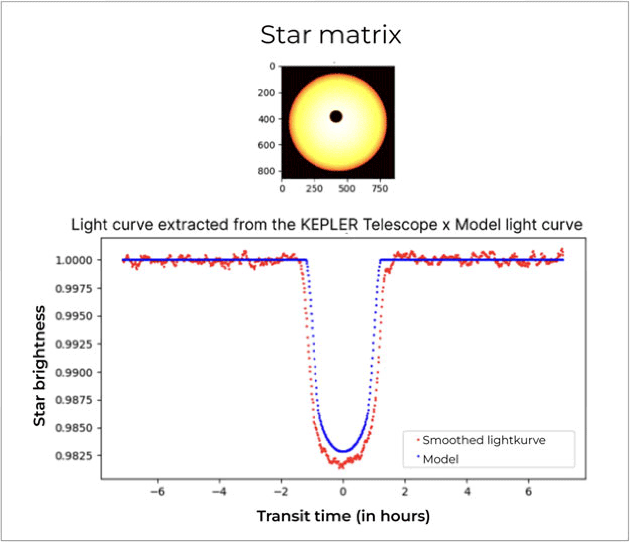
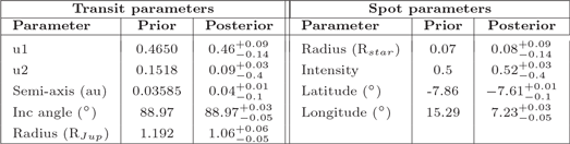
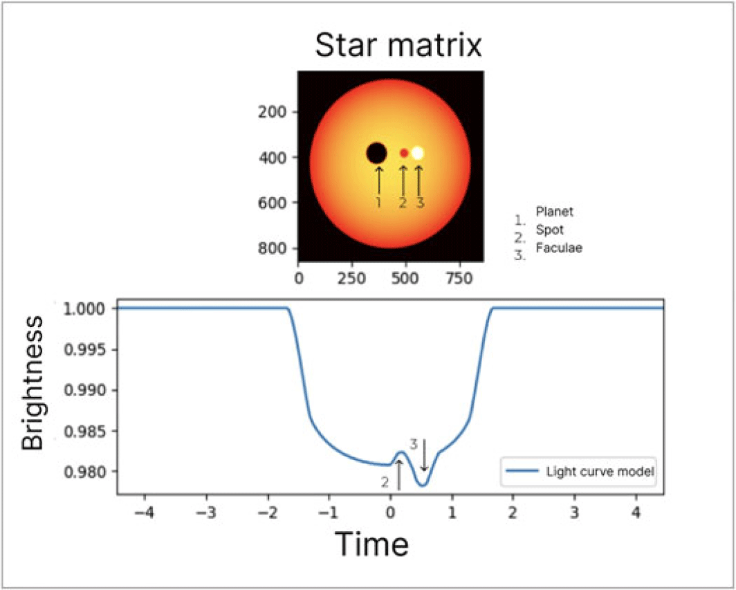
An example of the model (blue curve) is shown in Figure 1 where the parameters of the star Kepler-423 and the planet Kepler 423 b were sourced from Exoplanet.EU Extrasolar Planets Encyclopaedia (2024) and are listed as priors in Table 1. As can be seen, the parameters need improvement. A model of a star with a spot and a facula is shown in the right panel of Figure 2. The impact of these features on the light curve as they are occulted by the planet during its transit is indicated by the arrows.

Figure 1.

Kepler-423 light curve transit observed by the Kepler telescope (red) and the model of a spotless star using the parameters given in Extrasolar Planets Encyclopaedia (2024) (blue).

Table 1.

Results of MCMC fits

Table 1 Long description

A table comparing transit and spot parameters with prior and posterior values. The table has two main sections: Transit parameters and Spot parameters, each with three columns: Parameter, Prior, and Posterior. The Transit parameters section includes rows for u1, u2, Semi-axis, Inc angle, and Radius with their respective prior and posterior values. The Spot parameters section includes rows for Radius, Intensity, Latitude, and Longitude with their respective prior and posterior values. Each row lists the parameter name followed by its prior and posterior values.

Figure 2.

Transit simulation adding a planet (1), a spot (2), and a faculae (3), and their respective changes in the light curve, indicated by the numbered arrows.

For the fitting of the observed light curve with the ECLIPSE model, we integrated parallel C code into our Python scripts to accelerate matrix generation during MCMC sampling, resulting in a 50x to 80x performance gain Pinho, Silva & Valio (Reference Pinho, Silva and Valio2022). The MCMC method is advantageous as it not only fits the model to the data but also yields the uncertainties (upper and lower bounds) for each parameter.

3. Results: Fiting Star and Exoplanets Parameters and Spots

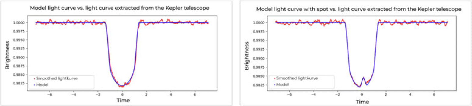
Figure 3 illustrates the complete fitting process. The left panel shows the initial fit of a spotless star model (blue) to the Kepler light curve (red), which determines the host star and planetary parameters (Table 1, third column). Then, these parameters are fixed while another MCMC fit models the stellar spot occultation, the results of which are plotted in the sixth column of Table 1. The result of this two-stage fitting process is a complete model (blue) that closely reproduces the observed Kepler data (red), as shown in the right panel of Figure 3.

Figure 3.

Left: Light curve resulting from the fitting of planet and star parameters (blue curve) compared to the curve downloaded from the telescope (red curve). Right: Light curve resulting from the fitting of the parameters of a spot (blue curve) compared to the curve downloaded from the telescope (red curve).