


Introduction
Worldwide, family and indigenous agriculture provide around 56% of basic food products but occupy barely 20% of the available arable land (Gornitzky, Reference Gornitzky2015), most of which is marginal in terms of yield potential of main crops. In the Northwest of Argentina (NWA), yields are limited by the natural conditions of the highlands (those located at least 1000 metres above the sea level, masl) characterised by low air temperature (T), which decreases with an average rate of 0.55°C for every 100 m (Körner, Reference Körner2003). On the contrary, in the NWA, solar radiation can be 30% higher during summer at 3350 compared with 1150 masl in locations at similar latitudes, partly due to increased UV (Utrillas et al., Reference Utrillas, Marín, Esteve, Salazar, Suárez, Gandía and Martínez-Lozano2018). Most cropped species in the NWA are maize, quinoa and Andean potato (www.siia.gov.ar) among which maize is the only one with a C4 photosynthetic metabolism, implying higher sensibility to low T but, at the same time, a higher response to increasing irradiances (Andrade, Reference Andrade1995; Muchow et al., Reference Muchow, Sinclair and Bennett1990). Available information regarding the compound effects of altitude on maize crops is scarce, and more studies are needed to develop specific management strategies for maize in these environments.
At increasing altitudes, the decrease in mean T implies a shortening of the frost-free period and a concomitant delay in sowing date, which reduces the crop cycle duration and, with this, the light interception throughout it. After sowing, low temperatures extend the duration in days of phenological stages (Ritchie and Hanway, Reference Ritchie and Hanway1989), with differences of up to 80 days in crop cycle duration between sites differing in 1000 m of altitude (Cooper, Reference Cooper1979). This implies a delay in achieving maximum leaf area index (LAI), resulting in further reductions in light interception and biomass accumulation with increasing altitude (Cooper, Reference Cooper1979; Pace, Reference Pace2019). At the same time, the decrease in T with increasing altitude will also extend the duration of the critical period, and with this, the light interception during this period could finally result in a larger grain number (Andrade et al., Reference Andrade, Vega, Uhart, Cirilo, Cantarero and Valentinuz1999). Consistently, increasing night T during the critical period (+5°C with maximum night T of 25°C) results in a shortening of this stage and a lower grain number (Cantarero et al., Reference Cantarero, Cirilo and Andrade1999).
Among the environmental factors affecting photosynthesis, low night temperatures can reduce maize photosynthesis by up to 30%, especially in the early morning (Kosová et al., Reference Kosová, Haisel and Tichá2005; Ying et al., 2000). Also, the lower atmospheric pressure typical of high-altitude environments can reduce the CO2 diffusion rates to chloroplasts (Körner, Reference Körner2007) and lower vapour pressure deficits (typical in the NWA) may promote stomatal closure regardless of the plant water status, implying CO2 limitations for photosynthesis even in C4 species (Hirasawa y Hsiao, Reference Hirasawa and Hsiao1999). On the other hand, higher irradiance with increasing altitude could represent an advantage for maize, whose photosynthesis at the leaf level saturates beyond 2000 μmoles photons m−2 s−1 (Chen et al., Reference Chen, Xiao, Chen, Li, Zhang, Chen, Yuan and Mi2014).
Part of these negative environmental effects could be mitigated by increasing plant density, which is an important management variable in maize (Maddonni et al., Reference Maddonni, Otegui and Cirilo2001; Tokatlidis and Koutroubas, Reference Tokatlidis and Koutroubas2004). A higher plant density could partially overcome the delayed crop phenology, allowing an earlier achievement of maximum leaf area index further benefitted from the larger radiation input, whereas detrimental effects over grain number could be compensated for by an extended duration of the critical period. The objective of this work is to evaluate canopy development, light interception, leaf traits, photosynthetic performance and yield of Andean maize cropped in highlands under contrasting plant densities.
Materials and Methods
Experimental design
Experiments were conducted in two sites of NWA located at different altitudes. One of the sites was in Hornillos (hereafter, HOR), Jujuy province, at 2380 masl (23.65° S. 65.43° W) within the Instituto de Investigación y Desarrollo Tecnológico para la Agricultura Familiar del Noroeste Argentino, IPAF NOA (Institute for Smallholders Agriculture of the Northwest of Argentina), which belongs to the Instituto Nacional de Tecnología Agropecuaria, INTA (National Institute of Agricultural Technology). The other site was in an annexed field of the elementary school at El Rosal (hereafter, ERO), Salta province, at 3350 masl (24.38° S. 65.77° W). At each site, treatments consisted of two contrasting planting densities: 5.7 and 8.6 plants m−2. The low density corresponded to the recommended density for these environments (Gómez and Macedo, Reference Gómez, Macedo and Minifundio2011) whereas 8.6 plants m−2 is 50% higher than recommended. An open-pollinated line called ‘creole yellow corn’ was sown at both sites and ‘white corn’ was also included at HOR. Both genotypes are usually cropped by farmers within this altitudinal range and have been widely known as local races (Cámara Hernandez et al., Reference Cámara Hernández, Miante Alzogaray, Bellón and Galmarini2011). Seeds were obtained from the INTA seed multiplication programme. Soil samples were taken at each site and classified as sandy loam at HOR and sandy at ERO (Suppl. Material Table S1). Both soils had high values of organic matter (>2.8%), and similar pH values and carbon/N relationships.
Crop management
Previous crop was Andean potato at ERO, quinoa and amaranth at HOR in the first season and maize at HOR in the second season. Approximately 30 days before sowing, dry goat guano was applied at an estimated rate of 1 kg m−2 in both sites, which is similar to rates used by local farmers (Gómez and Macedo, Reference Gómez, Macedo and Minifundio2011). Guano chemical composition was analysed in 2019 in the laboratory of the Universidad Nacional de Jujuy (National University of Jujuy), allowing to estimated rate of 187 kg ha−1 of nitrogen and 174 ppm of extractable phosphorus applied. Treatments were laid out in three blocks (four blocks in HOR in the second season) and densities were randomly distributed in plots within each block at each site. At HOR, genotypes were distributed in subplots within each plant density. Each plot (ERO) or subplot (HOR) consisted of 4 rows 0.7 m apart and 4 m long (11.2 m2). Seeds were sown manually on October 29th at HOR, October 31st at ERO in 2019 and December 2nd at HOR in 2020. Three seeds were placed on each hill and then thinned to the aimed density after emergence. The crop was maintained free of weeds and insects using conventional agrochemicals when necessary and was irrigated as needed from emergence using ditch irrigation at HOR and drip irrigation at ERO. Previous work indicates that nitrogen leaching is higher under ditch irrigation and water use efficiency is lower compared with drip irrigation (Li et al., Reference Li, Xiong, Cui, Huang, Xu, Han and Huang2020). However, these effects can be negligible in our work, since organic fertiliser was used (less prone to leaching) and water offered was enough to prevent water stress symptoms throughout the cycle.
Meteorological conditions
At HOR, T was registered by a meteorological station 100 m away from the experimental field. At ERO, T was registered by a thermocouple placed in a meteorological shelter; however, due to technical problems, gaps arose in the series of measured data. To fill these gaps, the hourly values estimated by the SOLCAST satellite database (https://solcast.com/) have been used, after a correction by linear approximation based on correlations between measured hourly T values and the SOLCAST values (only valid for summertime):
 $${{\rm{T}}_{{\rm{ERO}}}}\left( {^\circ {\rm{C}}} \right) = {\rm{1}}.{\rm{56}}\,^*\,{{\rm{T}}_{{\rm{SOLCAST}}}}\left( {^\circ {\rm{C}}} \right)-{\rm{1}}.{\rm{37}}$$
Solar radiation was also estimated using the SOLCAST model. Thermal time computations started at sowing, using mean daily air T and a base T of 8ºC (Ritchie and NeSmith, Reference Ritchie and Nesmith1991) whereas mean temperatures never exceeded the optimum T for maize growth (34ºC, Wilkens and Singh, Reference Wilkens and Singh2003). Thus, we used a simple linear model to calculate thermal time, which was expressed as the sum of ºC day−1 (Cd).
Non-Destructive determinations
In each site, 6 consecutive plants within the central rows of each plot were tagged at the V3 stage for non-destructive determinations. Crop phenology was determined in the tagged plants following the scale proposed by Ritchie and Hanway (Reference Ritchie and Hanway1989). Leaf area was assessed non-destructively by measuring the maximum length and width of each leaf and multiplying it by 0.75 as in Montgomery (Reference Montgomery1911) so that:
 $${\rm{Individual}}\,\,{\rm{leaf}}\,\,{\rm{area}} = {\rm{length}} \times {\rm{width}} \times 0.{\rm{75}}.$$
LAI was then calculated as the sum of the area of all the leaves of each plant multiplied by plant density. After flowering, a visual register of canopy senescence was done weekly and the area of senesced leaves (with more than 50% of its area yellowed) was subtracted from the LAI maximum achieved at flowering.
Chlorophyll content, specific leaf area and leaf N content
Different leaf traits were measured in leaves representing different canopy positions. The leaves measured were the third leaf above the main ear, representing an apical leaf, the leaf adjacent to the ear, representing a middle-positioned leaf, and the leaf positioned three leaves below the ear leaf, representing a basal leaf. In some plants, the earbud was still not visible by the time of sampling; in these cases the leaf below the topper-most expanded leaf was considered the apical leaf, going downwards every 3 nodes for middle and basal leaves. Chlorophyll content was assessed using a SPAD 502 (Minolta, EEUU). At least five measurements across the leaf blade were made and averaged, and three plants per plot (9 plants per treatment) were measured.
In these same leaf positions, specific leaf area was determined by punching 6 cm2 at the mid-third of each leaf thrice (i.e., 18 cm2 per leaf). Samples were obtained from 2 plants per plot (6 plants per treatment). Leaf discs were dried in an oven at 60ºC until constant weight and weighed. Specific leaf area was calculated as the quotient between the area of each leaf sample and the respective dry weight.
After specific leaf area was assessed, the same samples were utilised to determine leaf N content. A compound sample obtained from 2 plants per plot (3 replicates per each site × plant density × leaf position combination) was used for micro-Kjeldahl analyses using Hanon equipment (Nade, K9840) following conventional protocols for digestion and distillation of the samples.
Chlorophyll fluorescence measurements and stomatal conductance
Simultaneous photosynthetic electron transport rate (ETR) and stomatal conductance (gs) measurements were taken during 2 clear-sky days and at three times during the day: morning (09:00–11:00 hs), midday (12:00–14:00 hs) and afternoon (15:00–17:00 hs). Measurements were taken in apical, middle and basal leaves, representing different positions within the canopy (see above).
The effective photosystem II quantum yield was measured using a pulse-amplitude-modulated FMS2 chlorophyll fluorometer (Hansatech, UK). Each measurement was done in 3 plants per plot (9 plants per treatment) in fully illuminated spots around the middle position of the leaf lamina between the midrib and the leaf margin. Thus, measurements are an estimation of the photosynthetic potential of each leaf at each time of the day but do not account for differences related to varying irradiances throughout the day or across the canopy. Linear electron transport rate was calculated as in Rosenqvist and van Kooten (Reference Rosenqvist and Kooten2003):
 $${\rm{ETR}} = {\rm{PPFD}} \times {\rm{abs}} \times {\rm\varphi} {\rm{PSII}} \times 0.{\rm{5}}$$
where PPFD is the Photosynthetic Photon Flux Density, abs is leaf absorptance (0.8), ϕPSII is effective photosystem II quantum yield and 0.5 is a factor considering that 2 photons are absorbed by each transported electron (and assuming a 1:1 photosystem II/photosystem I ratio). The factor 0.8 (leaf absorptance) is typical for non-senescent leaves of maize (Acciaresi et al., Reference Acciaresi, Tambussi, Antonietta, Zuluaga, Andrade and Guiamet2014).
Stomatal conductance measurements were taken with a Porometer SC-1 (Decagon, USA) on the abaxial side of the leaf, in the same fully illuminated leaf spots used for ETR measurements.
Biomass, yield and yield components
In both seasons, destructive samplings were made at HOR at physiological maturity for dry matter determinations. In each subplot, 6 previously tagged plants were harvested and dissected in three parts: (i) stalks with leaf sheaths and tassels, (ii) leaf blades and (iii) ears. All parts were dried in a forced-air oven at 60°C to constant weight and weighed. Aboveground plant biomass was estimated as the sum of stalks, leaf blades and ears.
Yield was estimated by harvesting 20 ears from consecutive plants within the central rows of each plot. No barren plants were found in any of the experiments. Ears were threshed manually, grains were weighed and an aliquot was oven-dried to constant weight to calculate the percentage of grain moisture in order to express yield at 0% moisture. Mean individual kernel weight (KW) was estimated by counting and weighting grains of each plant harvested for biomass. Kernel number per plant (KNP) was estimated on the basis of KW and grain yield of 20 plants per plot.
Samplings in farmer’s fields
To complement the experimental results, during the 2022–23 growing season, samplings were carried out in 8 farmer’s fields across an altitudinal gradient spanning from 2400 up to 3400 masl, and within −23.20° and −24.41° latitude (Fig. S1). In all cases, yellow or white maize varieties were sown at conventional sowing dates, irrigated by furrow irrigation and fertilised with goat manure, and no evidence of nutritional or drought stress was observed by the time of visiting the fields. In each field, two separate plots with 4 rows and 1.5 m length were identified around flowering, aiming to represent a variation of plant densities. Plant density was separately estimated for each of the central rows of each plot by counting the total number of plants in the harvested row and the adjacent rows at each side and dividing it by the area occupied by these plants (i.e., 1.5 m length × 0.70 distance between rows × 3 rows). At maturity, all the ears in each of the central rows of each plot were separately harvested, threshed manually, dried until constant weight and weighed. The number of grains per ear was counted and the kernel weight was estimated on the basis of yield per plant and KNP. Thus, a maximum of 4 data of yield and plant density was available in each farmer field although for different reasons (usually bird attack) some plots were lost in some fields.
Statistical analyses
Data were analysed using the STATISTICA 7.1 Software (Stat-Soft, Inc., Tulsa, Oklahoma, USA). Treatments and interaction between them were analysed by ANOVA, and the Levene’s test was used to corroborate the assumptions of the model. Each site was analysed independently because of different measurement times except when specifically stated. Plant density, genotype (at HOR) and block were considered fixed factors and each independent variable was analysed separately. For variables comprising different leaves of the canopy or different moments during the day, the leaf position and/or the moment of the day were also treated as fixed factors. When interaction among factors was detected, the LSD test (p < 0.05) was used to identify homogenous groups. The significance of regressions was assessed through the F-test (p < 0.05).
Results
Environmental variation and phenological development
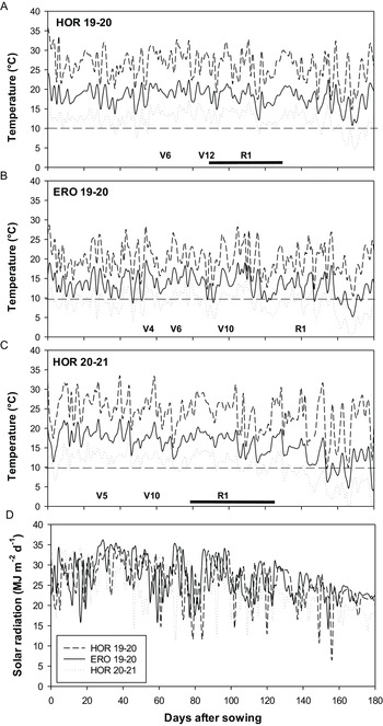
The increase in altitude from 2380 masl at HOR to 3350 at ERO implied an important decrease in T. During 2019–20, medium T during the first 150 days of the cycle was 33% higher at HOR compared with ERO (Fig. 1a, b) whereas differences in minimum T were even larger (+40% at HOR). Regarding chilling stress (<10°C, Waqas et al., Reference Waqas, Wang, Zafar, Noor, Hussain, Azher Nawaz and Farooq2021), during the first 150 days of the cycle, only 7 days with minimum T below 10°C were registered at HOR whereas, at ERO, there were 94 days out of 150 with minimum T below 10°C. Thus, at ERO, apart from lower medium T, plants may have also experienced critically low minimum temperatures. As expected, T differences delayed phenological development at the highest altitude site, ERO, where the crop reached silking 39 days later than at HOR in 2019–20 (Fig. 1a, b). Nonetheless, much lower thermal time was required to achieve a given phenological stage at ERO: for example, V6 was reached at 697°C.d at HOR but at 458°C.d at ERO. Thus, thermal time requirements were reduced when lower temperatures were experienced.
Temperatures during the growing cycle of Andean maize in Hornillos (2380 masl) during 2019–20 (A) and 2020–21 (C) and in El Rosal (3350 masl) during 2019–20 (B), and solar radiation (MJ m−2) in the three experiments estimated by the SOLCAST satellite database (D). Minimum, mean and maximum temperatures are indicated by dotted, solid and dashed lines, respectively, and the horizontal dashed lines mark the limit for temperatures below 10°C, potentially stressful for maize. Phenological stages, indicated above the ‘x’ axis, are defined based on the scale proposed by Ritchie et al. (1989). In Figures A and C, the black bar below R1 indicates the chronological time elapsed during the critical period estimated in 400°C bracketing silking (Sadras and Calderini, 2020).

Comparing both seasons at HOR, medium and minimum T were higher during the 2019–20 growing season compared with 2020–21, and this was accentuated during the reproductive stage (+16 and +22% higher medium and minimum T in 2019–20 averaged from silking until 40 days after silking, Fig. 1a, c). Cumulative solar radiation was also higher in the 2019–20 growing season, with 11% higher solar radiation accumulated until silking and 8% higher solar radiation accumulated from silking until maturity (Fig. 1d).
Leaf area index and light interception
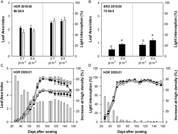
The increase in plant density increased LAI and light interception with varying intensity depending on the environment. During the first season at HOR, no significant effect of plant density was detected for LAI or light interception at 86 DAS (Fig. 2a), except for a minor advantage at 65 DAS (+17% higher LAI at high density, p < 0.1, not shown). By contrast, at ERO, the increase in plant density improved LAI by 75 DAS resulting in a 40% increase in light interception (Fig. 2b). Overall, individual leaf size was larger at ERO compared with HOR (Fig. S2), with a declining trend towards later-developed leaves. Thus, the increase in altitude drastically reduced the LAI achieved by the crop, but this was partially offset by the increase in plant density.
Leaf area index and light interception measured at midday in Andean maize at Hornillos (2380 masl) during 2019–20 (A) and 2020–21 (C, D) and at El Rosal (3350 masl) during 2019–20 (B) at different plant densities. In (A), measurements were done 86 days after silking (filled bars correspond to yellow corn, empty bars to white corn). In (B), measurements were done at 75 days after silking in yellow corn. In (C) and (D), circles denote low plant density (5.7 plants m−2), triangles denote high plant density (8.6 plants m−2), filled symbols denote yellow corn and empty symbols denote white corn. In (C) and (D), empty bars show the relative increase at high plant density compared with low plant density in both genotypes (as no density × genotype interaction for LAI or light interception).

During the 2020–21 growing season at HOR, the higher plant density significantly increased LAI of both genotypes from 28 DAS to 153 DAS (Fig. 2c). In relative terms, this increase was higher during early crop stages (>50% higher LAI until 50 DAS), was maintained around 40% thereafter and tend to diminish towards the end of the growing period due to more accelerated canopy senescence at higher plant density. Light interception at midday was significantly improved by plant density until 78 DAS, with no significant effects thereafter. This is consistent with the crop achieving LAI close to 4 by 80 DAS at the lower plant density, which is usually considered a critical value to maximise light interception in maize. Comparing genotypes, white corn achieved significantly higher LAI from 70 DAS onwards, regardless of plant density. However, light interception was slightly but significantly higher in yellow corn, from 64 DAS to 96 DAS, which related to a more planophile leaf habit in yellow corn (Fig. S3). Thus, increasing plant density beyond values conventionally used by farmers resulted in an important increase in LAI and light interception during early stages at ERO (3300 masl) and at HOR during 2020–21, but not at HOR during 2019–20 where highest temperatures during the vegetative period were experienced.
Leaf traits
Different leaf traits were analysed in 2019–20 around 96–98 DAS at both sites, allowing a representative statistical comparison. Specific leaf area differed between sites depending on the plant density, being significantly higher at HOR at high plant density with no differences between sites at low density (Table 1). The increase in plant density resulted in higher specific leaf area at HOR (i.e., thinner leaves), but, surprisingly, the opposite was true at ERO. Differences were also detected depending on the leaf position with generally higher specific leaf area at basal leaves (Table 1).
Specific leaf area (cm2 mgDW −1), SPAD values, N concentration (%) and N content (mg cm−2) of Andean maize at two locations: Hornillos (HOR, 2380 masl) and El Rosal (ERO, 3350 masl) during 2019–20. Leaf traits were measured under two contrasting plant densities (5.7 and 8.6 pl m−2), in 3 leaves representing different positions within the canopy (basal, mid and apical leaves). Statistical significance represented as: *: p < 0.05; **: p < 0.01 and ***: p < 0.001; NS indicates no significant relationship. For each trait, mean values for each significant factor are deployed

Leaf chlorophyll content was estimated on the basis of SPAD values (‘greenness’) and resembled the differences found for specific leaf area. Significantly higher SPAD values were achieved at ERO (in line with thicker leaves), whereas at HOR, the increase in plant density further reduced SPAD values, consistent with the increase in specific leaf area (i.e., thinner leaves) (Table 1). The SPAD value also changed significantly depending on the leaf position with generally lower SPAD values in apical leaves compared with leaves in middle or basal positions at both sites (Table 1).
Leaf %N and leaf N content were also significantly higher at ERO, with no interaction with plant density (Table 1). While higher leaf N content could be partially attributed to thicker leaves at ERO (+8% compared with HOR), relative differences were much greater for N content (+39% compared with HOR). At both sites, apical and middle-positioned leaves had higher N content than basal leaves (Table 1). Overall, several leaf traits differed between sites with a trend to thicker leaves, with higher chlorophyll and N content at the higher altitude site.
Photosynthetic rates and stomatal conductance
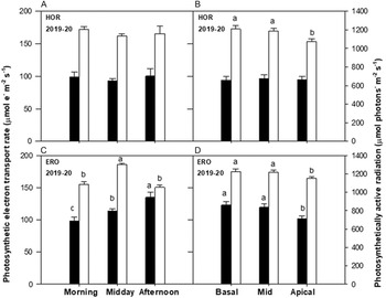
ETR and stomatal conductance (gs) were measured throughout the day in illuminated leaf spots of 3 leaves representing different positions within the canopy. Because ETR values are usually related to the incoming photosynthetically active radiation (PAR) at the site of measurement, PAR values were also registered but are not representative of the zenithal incoming PAR at those canopy levels or times of the day. Throughout the day, no variation was found at HOR (Fig. 3a) whereas at ERO, ETR was significantly lower in the morning, increasing by 15% at midday and by 37% in the afternoon, with no evident relationship with PAR (Fig. 3c). Regarding the leaf position, at HOR, ETR was significantly lower in the basal leaf at high plant density (72 vs. 99 μmoles e- m−2 s−1 for the rest of the leaves) but, except for this, no significant differences were detected between leaves, despite slightly higher (+11%) incoming PAR at basal and middle leaves (Fig. 3b). By contrast, at ERO, ETR was +19% higher in basal and middle leaves compared with apical leaves, which may partially relate to their +6% higher incoming PAR (Fig. 3d), likely related to the usually more planophile leaf angle. Comparing sites, ETR was higher at ERO than at HOR, especially at midday (+23%) and in the afternoon (+34%), and especially in low (+30%) and middle-positioned leaves (+24%) (based on comparisons in Fig. 3). Overall, a higher photosynthetic potential was achieved at ERO but also a much higher variation throughout the day.
Photosynthetic electron transport rate (μmoles e- m−2 s−1, filled bars) and photosynthetically active radiation (μmoles photons−1 m−2 s−1, empty bars) at the leaf spot where measurements were taken in Andean maize at Hornillos (2380 masl, a, b) and at El Rosal (3350 masl, c, d) during 2019–20. In each site, measurements were taken during 2 consecutive days, in the morning, midday and afternoon in plants grown under two contrasting plant densities (5.7 plants and 8.6 plants m−2) and in 3 leaves representing different positions within the canopy. Significant differences during the day are shown in A and C by pooling together plant densities and leaf positions, whereas significant differences between leaf positions are shown in B and D by pooling together plant densities and time of the day. Lines above the bars indicate the standard error and letters show homogeneous groups according to the LSD test (p < 0.05).

Stomatal conductance varied throughout the day at both sites. At HOR, gs was +44% higher in the morning than later in the day (Fig. 4a) with no apparent effect on ETR, which was unchanged throughout the day (Fig. 3a). Similarly, at ERO, gs decreased throughout the day with +53% higher gs at the morning and midday compared with the afternoon (Fig. 4c), with no evident relationship with ETR, which was highest in the afternoon (Fig. 3c). Regarding leaf position, at HOR, gs was +38% higher at mid and apical leaves compared with the basal leaf (Fig. 4b) but all the leaves achieved similar ETR (Fig. 3b). Also at ERO, gs was higher (+26%) at mid and apical leaves compared with the basal leaf (Fig. 4d) with no evident relationship with ETR, which was highest in basal and mid leaves (Fig. 3d). Thus, overall, ETR differences throughout the day and across leaf positions showed no evident relationship with gs variation.
Stomatal conductance (mmoles H2O m−2 s−1) at the same leaf spot where photosynthetic electron transport rate measurements were taken in Andean maize at Hornillos (2365 masl, a, b) and at El Rosal (3350 masl, c, d) during 2019–20. In each site, measurements were taken during 2 consecutive days, in the morning, midday and afternoon, in plants grown under two contrasting plant densities (5.7 plants and 8.6 plants m−2) and in 3 leaves representing different positions within the canopy. Significant differences during the day are shown in A and C by pooling together plant densities and leaf positions, whereas significant differences between leaf positions are shown in B and D by pooling together plant densities and time of the day. Lines above the bars indicate the standard error and letters show homogeneous groups according to the LSD test (p < 0.05).

Biomass, yield and yield components
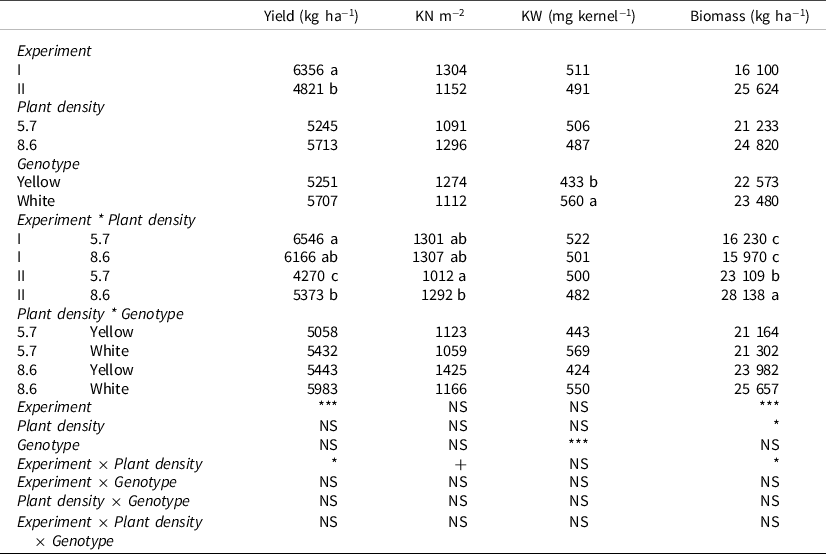
Biomass and yield data were obtained from two independent experiments at HOR. Between experiments, yields were 32% higher in the first season but this was not due to increased biomass accumulation, which was larger in the second season (+59%, Table 2). Between yield components, a non-significant trend showed that kernel number was more affected (−13%) than kernel weight (−4%) in the second season compared with the first season.
Yield (kg ha−1), kernel number (KN m−2), kernel weight (KW, mg kernel−1) and biomass (kg ha−1) in two genotypes of Andean maize (white and yellow corn) grown at Hornillos (HOR, 2380 masl) during 2019–20 and 2020–21 under two contrasting plant densities (5.7 and 8.6 pl m−2). Statistical significance represented as: +: p < 0.1; *: p < 0.05; **: p < 0.01 and ***: p < 0.001; NS indicates no significant relationship. For each trait, mean values for each significant factor or interaction among factors are deployed

Increasing plant density from 5.7 to 8.6 plants m−2 did not improve yield or modified yield components in 2019–20, whereas in 2020–21 a + 26% yield gain was obtained by increasing plant density in both genotypes (Table 2). This was related to a + 28% increase in kernel number that did not substantially affect kernel weight (−4%) and with +22% biomass accumulation. Comparing genotypes, white corn exhibited constitutively higher kernel weights and a non-significant trend to higher yields across seasons and plant densities (Table 2). Thus, yield benefits were obtained by increasing plant density in the second season, when overall lower temperatures were experienced and lower yields were attained.
Yield response to plant density in farmer’s fields
Plant density and yield data were also obtained from samplings in 8 farmer’s fields within an altitudinal range spanning from 2400 up to 3400 masl during the 2022–23 growing season. A wide range of plant densities were explored across farms, with a minimum of 6 and a maximum of 15 pl m−2. The expected significant relationship between plant density and yield per plant was found (Fig. 5a, r 2 = 0.57***). Based on the linear equation obtained from this relationship, it was possible to estimate an expected yield per plant at each density and with this an optimum yield of 3650 kg ha−1 was achieved at 10 pl m−2 (inset in Fig. 5a). Regarding yield components, kernel number m−2 was positively related to plant density (r 2 = 0.40**, Fig. 5b) with no evidence of stagnation even at 15 pl m−2. By contrast, kernel weight was negatively related to plant density (r 2 = 0.41**, Fig. 5c). Data belonging to highest altitude locations (empty symbols in Fig. 5) are usually located above the trend line in Fig. 5b and below the trend line in Fig. 5c, suggesting that, as altitude increases, increasing plant densities result in relatively higher gains in grains m−2 and higher penalties over kernel weight. Thus, in these high-altitude environments, kernel weight is the yield component clearly most affected by increases in plant density whereas no apparent detrimental effect is seen for kernel number even at very high plant densities as 15 pl m−2.
Results obtained from samplings in farmer’s fields during 2022–23 growing season: yield per plant (A), kernel number m−2 (B) and kernel weight (C) as a function of plant density (estimated by the number of plants in the sampled row and the adjacent rows at each side). Different symbols denote the altitude of each location, whereas each symbol represents the average value of each sampled row (1.5 m length). Inset in (A) shows the expected yield response based on the linear equation obtained between yield per plant and plant density. Asterisks denote significant regressions: **, p < 0.01; ***, p < 0.001.

Discussion
Phenological development
As expected, the lower temperatures associated with increased altitude at ERO had an important effect in delaying crop phenology, with 39 additional days being required to achieve R1 compared with HOR. Similarly, for landraces grown in Mexico in sites at 1550 and 2050 masl, up to 50 extra days were required to achieve the V16 stage at 2050 masl (Pace, Reference Pace2019). However, these extra days did not fully compensate for growing degree days: 297°C.d less was required to achieve the R1 stage at ERO compared with HOR in our work. Similarly, 200°C.d less was required to complete the crop cycle in sites with the same photoperiod and differing in only 400 m of altitude (Jiang et al., Reference Jiang, Edmeades, Armstead, Lafitte, Hayward and Hoisington1999). This is consistent with environmental modulation of the plastochron (Padilla and Otegui, Reference Padilla and Otegui2005) and the phyllocron in maize (Riva-Roveda et al., 2016; Tsimba et al., 2013a). The phyllocron is decreased with lower temperatures within the range of 12.5–25.5°C (explored in our study) and also by increased solar radiation (Birch et al., Reference Birch, Vos, Kiniry, Bos and Elings1998), whereas higher proportion of UV-B apparently does not affect development (Kakani et al., Reference Kakani, Reddy, Zhao and Sailaja2003). Overall, the increase in altitude delayed phenological development but also, drastically reduced the thermal time requirements in the maize genotype studied in our work.
Leaf area index and light interception improved at higher density
Leaf area index and light interception were greatly reduced at the highest altitude site in line with previous reports (Cooper, Reference Cooper1979). While both delayed phenological development and reduced leaf size could account for these differences, here, leaf size was higher at ERO, at least for early-developed leaves (Fig. S2), which has been explained as a result of prolonged duration of leaf expansion (Cooper, Reference Cooper1979; Laffitte and Edmeades, Reference Lafitte and Edmeades1997). Nonetheless, very low temperatures were explored in our work at the highest altitude site (>90 days with minimum T below 10°C during the vegetative period, Fig. 1b) and relatively mild chilling temperatures (14/10°C) can reduce leaf size both through effects over cell division and expansion (Louarn et al., Reference Louarn, Andrieu and Giauffret2010). Thus, both effects, prolonged duration of leaf expansion and chilling affecting leaf expansion are likely interacting in opposite directions, finally increasing (as here) or decreasing leaf size at higher altitudes.
The increase in plant density improved light interception by 75 DAS at ERO (Fig. 2b), and until 78 DAS at HOR in the second season (Fig. 2d), which coincided with the crop achieving a LAI of 4 at low density (Fig. 2c), around the critical value for maize. Lower temperatures during the vegetative period at ERO (Fig. 1b), or a shorter vegetative period at HOR also combined with slightly lower temperatures (Fig. 1c), limited canopy development allowing plant density advantages in LAI and light interception to be expressed. By contrast, during 2019–20 at HOR, higher temperatures and a longer duration of the vegetative period (Fig. 1a) allowed a larger canopy to be developed, with no advantages of increased plant density related to a trend to reduced leaf size (not shown). Previous works have shown that leaf size is reduced with increasing plant density, but still, LAI usually increases up to 10–12 plants m−2 except in very specific genotype × environment combinations (Madonni et al., Reference Maddonni, Otegui and Cirilo2001). Thus, in these high-altitude environments, increasing plant density can improve LAI and light interception during the vegetative period, especially under cooler temperatures (ERO 2019–20) or shorter vegetative periods (HOR 2020–21) than those experienced at HOR 2019–20.
Leaf traits
Many leaf traits changed between sites and plant densities. Overall, thicker leaves were attained at ERO (at high density, Table 1), which was not an outcome of decreased leaf size (Fig. S2). Consistent with this, specific leaf area is decreased in leaves developed at low T (Riva-Roveda et al., Reference Riva-Roveda, Escale, Giauffret and Périlleux2016; Zhou et al., Reference Zhou, Zhou, He, Zhou, Ji and Zhou2020) and in maize lines from cool temperate regions compared with lines from warmer origin (Verheul et al., Reference Verheul, Picatto and Stamp1996). Increased light penetration in the canopy could explain the thicker leaves at ERO, whereas, at HOR, increased shading resulted in higher specific leaf area (Yabiku et al., Reference Yabiku, Akamatsu and Ueno2020) further augmented by high plant density (Table 1) in line with other works (Yang et al., Reference Yang, Chen, Xian and Chen2022). Other factors could also be involved, such as increased leaf sugar accumulation and decreasing specific leaf area which has been reported in leaves developed under lower T (Riva-Roveda et al., Reference Riva-Roveda, Escale, Giauffret and Périlleux2016).
Higher SPAD values (+36%) and N contents on a dry mass basis (+39%) were achieved at ERO compared to HOR (Table 1), which was not simply an outcome of thicker leaves since relative differences for specific leaf area were much lower (8% higher at HOR). Low temperatures usually decrease chlorophyll and N content in maize (Nie et al., Reference Nie, Robertson, Fryer, Leech and Baker1995; Leipner et al., Reference Leipner, Fracheboud and Stamp1997; Pasini et al., Reference Pasini, Bruschini, Bertoli, Mazza, Fracheboud and Marocco2005) and thus are unlikely to explain differences between sites in our work. By contrast, increased exposure to UV-B radiation results in higher chlorophyll concentration (Jovanić et al., Reference Jovanić, Radenković, Despotović-Zrakić, Bogdanović and Barać2022; Zancan et al., Reference Zancan, Cesco and Ghisi2006) and leaf protein concentration (Tevini et al., Reference Tevini, Iwanzik and Thoma1981), although these works did not explore the interaction with low T. Further work is needed to better assess the potential effects of UV-B radiation combined with lower temperatures over leaf traits, using realistic conditions as found in a high-altitude environment as ERO. In any case, thicker leaves, with higher protein content as found in ERO, could partially compensate for the decreased LAI with a higher photosynthetic potential.
Photosynthesis and stomatal conductance
Photosynthesis was estimated through ETR, which in C4 species correlates closely with CO2 assimilation (Earl and Tollenaar, Reference Earl and Tollenaar1999). Because our measurements were made at full irradiance, the ETR obtained here is a proxy of the photosynthetic potential of the leaves in each treatment and condition. At HOR, ETR was unchanged throughout the day (Fig. 3a) with minimum T during the days of measurement always above 15°C (Fig. 1a). By contrast, at ERO, ETR progressively increased throughout the day, with 37% higher ETR in the afternoon compared with the morning (Fig. 3c) and minimum T during the days of measurements below 8.3°C (Fig. 1b). Consistent with this, low night T (<10°C) can reduce maize photosynthesis by up to 30% (Dwyer and Tollenaar, Reference Dwyer and Tollenaar1989; Ying et al., Reference Ying, Lee and Tollenaar2000), chlorophyll fluorescence parameters such as ETR being directly affected (Ying et al., Reference Ying, Lee and Tollenaar2000). On the basis of maximum ETR achieved at each site, leaves at ERO showed a higher photosynthetic potential and no penalties for increased plant density.
Our results also suggest that the rate of recovery from low night T could be slow at high-altitude sites such as ERO (highest ETR in the afternoon, Fig. 3c), with implications over photosynthetic water use efficiency (i.e. the quotient between photosynthesis and transpiration rate), as at the same location, maximum gs was achieved in the early morning (+60% compared with the afternoon, Fig. 4c). Exploring genotypic differences in rates of recovery from low night T deserves further attention considering the potential implications on water use efficiency in these irrigated cropping systems. On the other hand, our results show that highest ETR rates were achieved at the highest altitude site (Fig. 3a vs. 3c in the afternoon) at very similar stomatal conductance rates (Fig. 4a vs. 4c in the afternoon), suggesting that the decrease in CO2 partial pressure with increasing altitude (Körner, Reference Körner2007) was not a major constrain here.
Biomass, yield and yield components
It is generally accepted that environments with a higher yield potential require higher planting densities to optimise yields (Tokatlidis et al., Reference Tokatlidis, Has, Melidis, Has, Mylonas, Evgenidis, Copandean, Ninou and Fasoula2011). However, there are some exceptions to this rule. For example, in late sowings, maize yields are usually decreased but optimum plant density can be similar or even higher compared with earlier sowings (Djaman et al., 2022; Zhai et al., 2021). In our work, higher yields were achieved in the first experiment at HOR but no response to plant density was obtained (6356 kg ha−1, Table 2), whereas in the second experiment, a later sowing date combined with cooler temperatures and lower solar radiation likely resulted in lower yields (4821 kg ha−1, Table 2) but also in a positive response to increased plant density (+26% in both genotypes). Results obtained from farmer’s fields (between 2400 and 3400 masl, thus higher than HOR) showed a consistent response of yield per plant to increasing plant densities (Fig. 5a), with an estimated maximum yield of around 3600 kg ha−1 being achieved at 10 pl m−2 (inset in Fig. 5a). Thus, environments with a lower yield potential (either in our second experiment or in farmer’s fields) seemed to benefit by increases in plant density.
The yield improvement at high planting density in the second season was mostly related to kernel number m−2 (+28%) (Table 2) and was consistent with the larger LAI and light interception achieved before flowering at high density (Fig. 2c, 2d). Similarly, across farmer’s fields, kernel number m−2 steadily increased with higher plant density (up to 15 pl m−2), with higher altitude locations being usually above the trend line (Fig. 5b). Benefits from increasing plant densities may be, thus, larger under higher altitudes (as it occurs in cool environments, Westgate et al., Reference Westgate, Forcella, Reicosky and Somsen1997), improving radiation interception during the critical period, and with this, kernel number (Andrade et al., Reference Andrade, Vega, Uhart, Cirilo, Cantarero and Valentinuz1999). On the other hand, reductions in kernel number at low planting density could be compensated for by larger kernels. But this was not observed, either in our second experiment (Table 2) or across farmer’s fields, where at low planting densities, empty symbols (obtained from higher altitudes) usually located below the trend line (lower ability to compensate low planting densities with higher grain weights, Fig. 5c). According to Zhou et al. (Reference Zhou, Yue, Sun, Ding, Ma and Zhao2017), low minimum T (<20.7°C) during grain filling combined with a high daily thermal amplitude (T max-min > 7°C) can decrease kernel growth rate. In our second experiment, minimum T during the first 30 days after silking was much lower than these (<10.8°C) and the daily thermal amplitude was much higher (T max-min > 12°C). The same can be speculated for the higher altitude locations where samplings in farmer’s fields were carried out. Consistently, dry matter remobilisation from vegetative parts is affected when ear T drops below 16°C (Setter and Flannigan, Reference Setter and Flannigan1986), possibly explaining the coexisting low yields with high biomass accumulation in the second season. Thus, increasing plant density could be a promising strategy for improving yields in high-altitude environments. Further research is needed to understand mechanisms behind penalties on kernel weight; especially, whether higher kernel number can improve biomass allocation to the ear under low temperatures that limit kernel growth rates.
Concluding remarks and future prospects
In this work, we show that increased altitude in mid-latitude environments of the Northwest of Argentina (3350 masl compared to 2300 masl) drastically delays phenological development, reduces thermal time requirements and modifies leaf traits increasing leaf thickness and leaf nitrogen content. Whereas a higher photosynthetic potential could be achieved at the highest altitude site this may not be fully exploited due to inhibitory effects of low night T and, apparently, long times of recovery from night chilling. Yield data obtained from experiments at 2300 masl and across farmer’s fields within 2400 and 3400 masl indicate that increased plant density beyond those currently recommended could potentially improve yields regardless of the environmental yield potential, with maximum yields of 3650 kg ha−1 achieved at 10 pl m−2. The main penalties of increased plant densities are related to reductions in kernel weight. Further work is needed to explore the effects of different factors limiting kernel growth rates, such as low temperatures and early frosts, over plant density responses.
Supplementary material
To view supplementary material for this article, please visit https://doi.org/10.1017/S0014479723000194
Acknowledgements
We thank Aldo Palacios, Director of the School at El Rosal, for providing the piece of land for field trials. We are also grateful to the support staff at IPAF for helping with the crop management. We are deeply thankful to the farmers who kindly allowed us to carry out the samplings in their fields, who are, right now like many others, standing up for their ancestral territories under the threat of uncontrolled lithium business.
Financial support
This work was partially funded by the Consejo Nacional de Investigaciones Científicas y Tecnológicas, CONICET (National Council of Scientific and Technological Research, PIP 11220210100007) and by the FAO Project PR-154, Fondo de Distribución de Beneficios del Tratado Internacional sobre los Recursos Fitogenéticos para la Alimentación y la Agricultura, TIRFAA (Benefit-sharing Fund of the International Treaty on Plant Genetic Resources for Food and Agriculture).
Competing interests
The authors declare none.