


Introduction
Racial representation gaps persist in elected offices across all levels of government in the United States. Although nonwhite individuals comprise approximately 40% of the US population, they account for only 26% of voting members in the 119th Congress.Footnote 1 While this marks the most racially and ethnically diverse Congress to date, a significant disparity remains. At the state level, the National Conference of State Legislatures (NCSL) reports an average gap of −6.57 percentage points between the proportion of nonwhite legislators and the nonwhite population in 2024.Footnote 2 Similarly, at the municipal level, Ricca and Trebbi (Reference Ricca and Trebbi2022) find that nonwhite minorities are collectively underrepresented by approximately 8.4 percentage points on city councils.
What are the drivers of the racial representation gap? This question can be answered from the demand perspective by asking how racial attitudes and behaviors among voters restrict minority office-holding (Citrin, Green, and Sears Reference Citrin, Green and Sears1990; Kam Reference Kam2007; McDermott Reference McDermott1997; Telles, Sawyer, and Rivera-Salgado Reference Telles, Sawyer and Rivera-Salgado2011), and from the supply perspective by exploring if minorities are underrepresented because of differences in candidate entry (Canon Reference Canon2020; Fox and Lawless Reference Fox and Lawless2005; Shah Reference Shah2014).
This article focuses on the supply side of the racial representation gap. In part to yield a comparable sample for the sake of causal inference, I examine individuals who have already demonstrated an interest in elected office – specifically, those who have previously run for office. The path to political office is shaped not only by ambition, which is reflected in advancement to higher office, but also by persistence. On one hand, candidates may choose to exit politics following a defeat, and racial differences in such decisions influence long-term patterns of racial representation. On the other hand, among those who win, the capacity to withstand political pressures and continue seeking reelection plays a critical role in sustaining office-holding. Thus, disparities in electoral persistence, specifically differences in the likelihood of rerunning, may either widen or help close the racial representation gap.
I use a close-election regression discontinuity design (RDD) and heterogeneous treatment effects by race to investigate whether nonwhite and white candidates make different choices in response to electoral outcomes. Additionally, I assess how rerunning decisions influence subsequent office-holding, shedding light on the role of electoral persistence in shaping racial representation.
Using 4,617 marginal candidates from city council elections in California, my results show that among narrowly losing candidates, nonwhite candidates are more likely to rerun for office than white candidates (25.7 vs. 16.2 percentage points). Overall, nonwhite candidates are 59% more likely to run again after a narrow loss. In contrast, among narrowly winning candidates, there is no racial difference in the likelihood of seeking reelection. The possibility of winning the subsequent election remains the same for all rerunning candidates. As such, the persistence of losing nonwhite candidates contributes to closing the racial gap. Occupational background analyses suggest that this persistence is primarily driven by candidates with public or community service experience.
Understanding the determinants of representation at the local level is essential because descriptive representation shapes outcomes in political development (Banducci, Donovan, and Karp Reference Banducci, Donovan and Karp2004; Gleason and Stout Reference Gleason and Stout2014; Grumbach and Sahn Reference Grumbach and Sahn2020), education (Kogan, Lavertu, and Peskowitz Reference Kogan, Lavertu and Peskowitz2021), labor market outcomes (Nye, Rainer, and Stratmann Reference Nye, Ilia Rainer and Stratmann2015), housing (Beach et al. Reference Beach, Jones, Twinam and Walsh2018), and policing (Bulman Reference Bulman2019; Christiani et al. Reference Christiani, Shoub, Baumgartner, Epp and Roach2022; Sass and Mehay Reference Sass and Mehay2003). Local office is also a key entry point for higher political careers (Frendreis, Gibson, and Vertz Reference Frendreis, Gibson and Vertz1990).
This article provides causal evidence on racial differences in political trajectories among individuals who seek office. First, while prior research focuses on ambition, whether winning candidates pursue a higher office (Shah Reference Shah2015), this article examines persistence by studying whether candidates continue seeking office after electoral wins or losses. Second, although prior scholarship finds mixed evidence on gender differences in electoral reentry (Bernhard and de Benedictis-Kessner Reference Bernhard and de Benedictis-Kessner2021; Thomsen and King Reference Thomsen and King2020; Wasserman Reference Wasserman2018), little research has been conducted on racial differences. Notably, studies on gender suggest that women, as the underrepresented group, are either no more likely or less likely to rerun than men. In contrast, this article presents an opposing pattern in the context of race, highlighting the greater persistence of nonwhite candidates.
Framework
This study estimates racial differences in candidates’ responses to electoral outcomes and future officeholding. A simple comparison of the future political involvement of all candidates could lead to biases due to unobserved candidate characteristics that are closely correlated with electoral outcomes. To isolate the causal effect of an electoral result from these unobserved characteristics, this study employs a close election RDD, following Lee (Reference Lee2008). This method restricts the comparison to candidates in tightly contested elections – where outcomes are largely determined by chance. Specifically, the analysis compares only the last-placed winners with the first-placed losers, reducing concerns that differences between competitive and noncompetitive candidates drive the results. Because identification in an RDD relies on local randomization around the cutoff, additional covariates are not required for identification, although predetermined covariates may improve estimation precision. Accordingly, the models do not include additional candidate-level covariates, which are not consistently available across candidates.
The main outcome variable is whether an individual runs for the city council election again in the subsequent election cycle (four years later). The running variable is the marginal vote share (MVS) for candidate
$ i $
 in election year
$ t $
 , denoted as
$ {MVS}_{it} $
 , which for winning (losing) candidates is the difference between their vote share and that of the first loser (last winner). The effect of losing an election on subsequent political participation can be written as

where
$ {Y}_{i,t+4} $
 represents whether candidate
$ i $
 runs for office again in four years. The parameter
$ \tau $
 represents the deterrence effect, capturing the discontinuity in the probability of running again at the margin of electoral victory. Assuming narrowly winning and losing candidates are otherwise similar, this approach provides a causal estimate of how an electoral outcome influences the likelihood of running for office again.
This study examines racial differences separately among narrow winners and losers. For winners, I assess whether there are racial disparities in the likelihood of seeking reelection. Similarly, for losers, I evaluate whether there are racial differences in candidates’ decisions to exit politics. This results in four key theoretical parameters at the threshold: the probability of rerunning for (1) nonwhite winners, (2) white winners, (3) nonwhite losers, and (4) white losers.
The empirical analysis estimates the effects using the following regression model:

where
$ {Lost}_{it} $
 is an indicator variable equal to 1 if the candidate
$ i $
 lost the election in year
$ t $
 .
$ \beta $
 captures the effect of losing on future political participation for white candidates.
$ \gamma $
 measures the difference in political persistence between nonwhite and white candidates among narrow winners.
$ \delta $
 represents the additional impact of an electoral loss on nonwhite candidates relative to white candidates. The function
$ f\left({MVS}_{it}\right) $
 allows MVS trends to vary across race and electoral outcome groups.
Results
Data and descriptive statistics
The main data source for this article is the California Elections Data Archive (CEDA), which compiles local election returns across California municipalities.Footnote 3 The election data cover the period from 1995 to 2014 and include 54 counties and 470 municipalities.Footnote 4 Election returns include candidates’ full name, ballot designation, incumbency status, election date/location, number of votes earned, total votes, number of individuals to be elected for a given office, and whether the candidate was elected.
CEDA data lack demographic information. To address this limitation, Beach and Jones (Reference Beach and Jones2017) collected the ethnicity information by (1) contacting the cities, (2) consulting ethnic organizations which maintain lists of government officials that are of Hispanic or Asian origin, and (3) coding candidate photographs using Amazon Mechanical Turk (MTurk).Footnote 5 MTurk classifications were validated using overlapping city-provided data,Footnote 6 and Sumner, Farris, and Holman (Reference Sumner, Farris and Holman2020) find that similar MTurk-based coding procedures produce highly accurate classifications. I obtained the candidate-level ethnicity data directly from the authors.
The primary outcome is whether an individual runs for the city council election again in four years. Since the final election cycle analyzed is 2014, any observations of individuals running for office in 2011 and later are dropped because it is unclear whether they rerun for office.
To implement the close election RDD, I limit the candidates to those who are the last-placed winners and the first-placed losers. Therefore, I only analyze races where the number of candidates exceeded the number of open seats.Footnote 7 The running variable for this analysis is margin vote share. Winning candidates have a positive margin vote share, which is calculated as the difference between their vote share and that of the first-placed loser. Losing candidates have a negative margin vote share, which is calculated as the difference between their vote share and that of the last-placed winner.
The final sample contains 4,617 marginal candidates. White candidates account for approximately 74% of the sample, while Hispanic, Black, and Asian candidates represent 18%, 5%, and 3%, respectively. Given this imbalance, fully disaggregating the main analysis would substantially reduce statistical power, particularly for Black and Asian candidates. Accordingly, the primary analysis classifies candidates into two categories: white alone (white) and not white alone (nonwhite). This classification is consistent with the article’s focus on the persistence of candidates from historically underrepresented racial and ethnic groups relative to white candidates.
Panel A of Table 1 presents summary statistics for all marginal candidates. Among these candidates, 56.9% of nonwhite candidates and 60.2% of white candidates were elected. Approximately, 45% of marginal candidates reran for office and 33.1% held office four years later. Of the 2,077 rerunning candidates, white candidates have an election rate of 75.4% in phase t + 4, while nonwhites have a rate of 67.9%. Panel B of Table 1 presents the summary statistics of close marginal candidates whose MVS is less than 11.2 percentage points, the optimal bandwidth.Footnote 8 The patterns are similar to those in Panel A.
Summary statistics

Table 1. Long description
The table is divided into two main sections: Panel A for Marginal candidates (columns 1 to 3) and Panel B for Close marginal candidates (columns 4 to 6). Each panel is further subdivided into All, Nonwhite, and White categories.
Main Data Rows:
* Elected in t: Values range from 0.557 to 0.602 across all categories.
* Rerun in t plus 4: Values range from 0.437 to 0.469.
* Elected in t plus 4: Values range from 0.314 to 0.336.
* Number of observations: Panel A has 4,617 total (1,183 Nonwhite, 3,434 White). Panel B has 3,421 total (811 Nonwhite, 2,610 White).
* Nonwhite share: 25.6 percent in Panel A and 23.7 percent in Panel B.
Conditional on rerun subsection:
* Elected in t plus 4: Values are higher, ranging from 0.674 to 0.754.
* Number of observations: 2,077 in Panel A (546 Nonwhite, 1,531 White) and 1,520 in Panel B (380 Nonwhite, 1,140 White).
* Nonwhite share: 26.3 percent in Panel A and 25.0 percent in Panel B.
Note: This table shows summary statistics for the marginal candidates who are the last-placed winners and first-placed losers in Panel A, and close marginal candidates whose marginal vote share is within 11.2 percentage points.
Main results
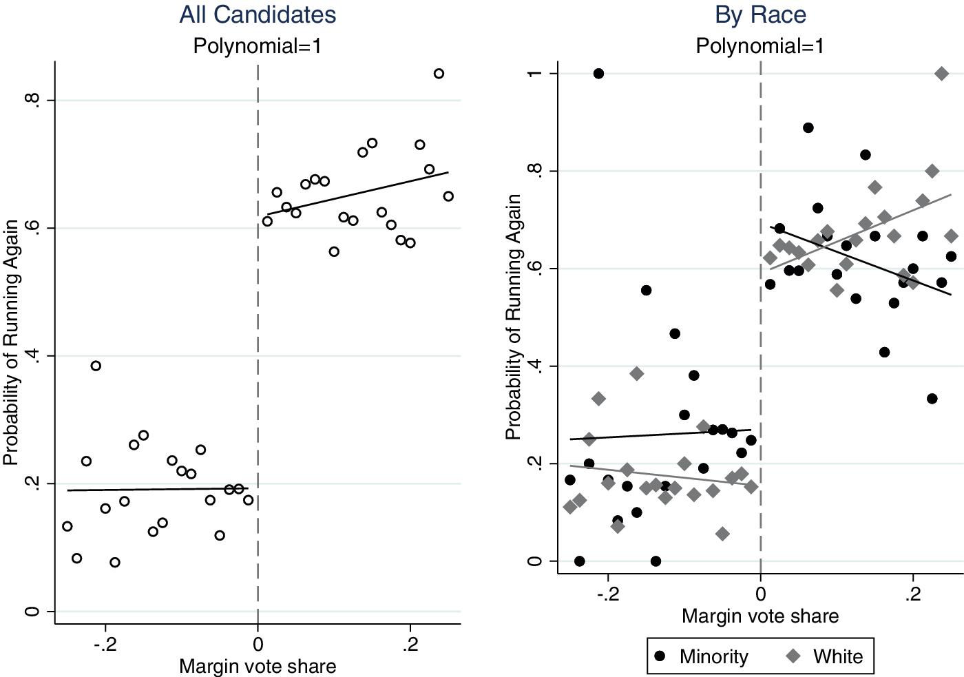
The left panel of Figure 1 presents graphical evidence of the effect of losing on subsequent political participation. The graph plots candidates’ probability of running for office in year
$ t+4 $
 against their MVS in year
$ t $
 . The dotted vertical line at zero represents the winning threshold. Candidates to the right of the threshold won their elections in
$ t $
 , while those to the left lost. A second-degree polynomial is fit on each side of the cutoff. Both sides exhibit relatively flat trends, with a clear discontinuity of approximately 40 percentage points at the threshold. This jump reflects the deterrence effect of electoral defeat, a component of incumbency advantage discussed by Lee (Reference Lee2008).
Effect of electoral outcome and race on subsequent political participation.

Figure 1. Long description
Two scatter plots with a vertical dashed line at zero on the x-axis representing the win or loss threshold.
Left Panel: Marginal Candidates.
* X-axis: Margin of Victory ranging from negative 0.2 to positive 0.2.
* Y-axis: Probability of Running Again ranging from 0 to 0.8.
* Data: Open circles show a cluster between 0.1 and 0.3 probability for losers (negative margin). There is a significant vertical jump at the zero threshold. For winners (positive margin), the probability clusters higher, between 0.6 and 0.8. Regression curves show a slight concave shape on both sides of the threshold.
Right Panel: Marginal Candidates by Race.
* X-axis: Margin of Vote Share ranging from negative 0.2 to positive 0.2.
* Y-axis: Probability of Running Again ranging from 0 to 1.
* Legend: Black dots represent Nonwhite candidates; grey diamonds represent White candidates.
* Data: For losers (negative margin), Nonwhite candidates show higher variance and a slightly higher average probability (peaking near 0.3) compared to White candidates (peaking near 0.2). For winners (positive margin), both groups jump to a probability between 0.6 and 0.8. The regression curve for White winners shows a steady upward trend, while the curve for Nonwhite winners peaks early and then declines slightly as the margin of victory increases.
The right panel of Figure 1 presents the main results of this article. It divides the sample by the candidates’ race. Nonwhite candidates are represented by black dots in bin scatter (bins of width equal to 0.0125 percentage points) and black fitted lines, while white candidates are represented by gray solid diamonds in bin scatter and gray fitted lines. For both groups, there is a discontinuity at the threshold that is consistent with the jump observed for all candidates in the left panel. At the winning threshold, where the gray vertical line intersects with the winning (right) fitted lines, there is no racial gap for future political involvement. However, at the losing threshold, visual evidence shows that nonwhite candidates are more likely to rerun for office compared to their white counterparts. As a robustness check, the linear fit shown in Figure A1 is consistent with the non-linear fit graph. Table A1 reports the corresponding regression estimates.
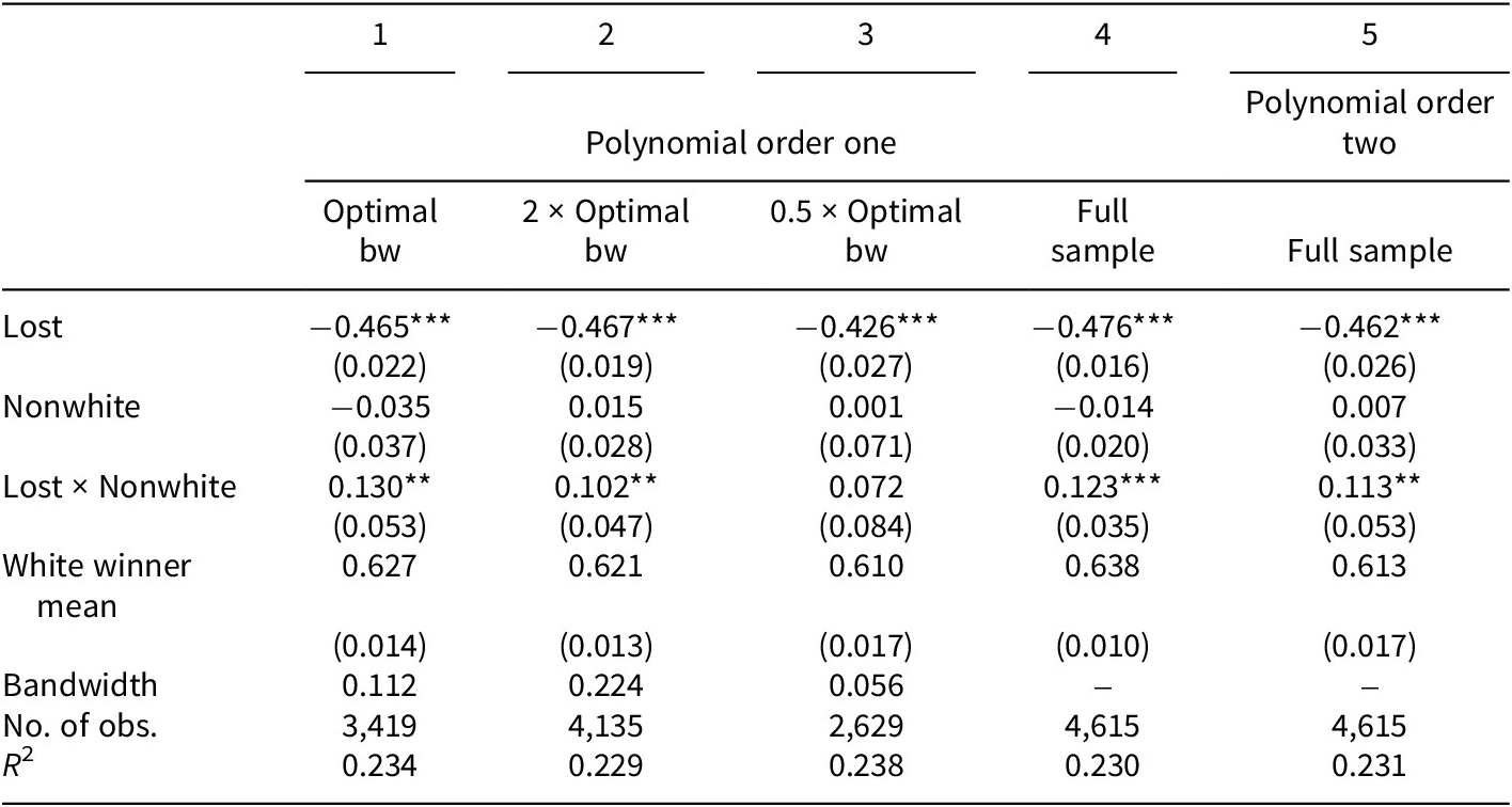
Table 2 presents estimates from Equation (2), corresponding to the right panel of Figure 1. The outcome variable is whether a candidate runs again for office in four years. Optimal bandwidths are selected separately for each panel, following Calonico, Cattaneo, and Titiunik (Reference Calonico, Cattaneo and Titiunik2014). County and year fixed effects are included in each specification, and standard errors are clustered at the county level. Columns 1–4 use a local linear regression with a first-order polynomial in the running variable. MVS and samples are restricted by various bandwidths around the cutoff for winning. Column 1 uses the optimal bandwidth; Columns 2 and 3 use twice and half that bandwidth, respectively. Column 4 uses the sample of all marginal candidates, without restriction on the range of MVS. Column 5 estimates a second-order polynomial using the full sample.
Effect of electoral outcome and race on subsequent political participation

Table 2. Long description
The table presents regression results for five models. Columns 1 through 4 use Polynomial order one, while Column 5 uses Polynomial order two. The bandwidths vary: Column 1 uses Optimal bw, Column 2 uses 2 times Optimal bw, Column 3 uses 0.5 times Optimal bw, and Columns 4 and 5 use the Full sample.
Key variables and their coefficients (standard errors in parentheses):
* Lost: Values range from minus 0.426 to minus 0.476, all significant at p < 0.01.
* Nonwhite: Values range from minus 0.035 to 0.015, none are statistically significant.
* Lost times Nonwhite: Coefficients are 0.130 (p < 0.05) in Model 1, 0.102 (p < 0.05) in Model 2, 0.072 in Model 3, 0.123 (p < 0.01) in Model 4, and 0.113 (p < 0.05) in Model 5.
* White winner mean: Values range from 0.610 to 0.638.
* Bandwidth: 0.112 (Model 1), 0.224 (Model 2), 0.056 (Model 3).
* Number of observations: 3,419 (Model 1), 4,135 (Model 2), 2,629 (Model 3), 4,615 (Models 4 and 5).
* R super 2: Values range from 0.229 to 0.238.
Note: The outcome variable is whether a candidate runs again for office in four years. Standard errors are clustered at the county level. County and year fixed effects are included.
Note: The outcome variable is whether a candidate runs again for office in four years. Standard errors are clustered at the county level. County and year fixed effects are included in each specification. Significance levels are indicating as: ***p<0.01, **p<0.05, *p<0.1.
The results are highly consistent across specifications. The coefficient on Lost (
$ {\beta}_1 $
 ) indicates that losing an election reduces the probability of rerunning by approximately 43–48 percentage points among white candidates. This deterrence effect has been well documented in prior literature, often discussed under related concepts such as incumbency advantage or the “scare-off” effect. The underlying logic is that the costs of running for office are substantially lower for incumbents, who benefit from greater resources, institutional advantages, and media exposure (Mondak Reference Mondak1995; Stone et al. Reference Stone, Fulton, Maestas and Maisel2010). As a result, losing candidates face a significant increase in the expected costs of running again, leading to a substantial drop in rerunning probability. The magnitude of the deterrence effect estimated in this article is large but consistent with prior findings. For example, Lee (Reference Lee2008) documents a deterrence effect of approximately 43 percentage points in US House elections. Similarly, Bernhard and de Benedictis-Kessner (Reference Bernhard and de Benedictis-Kessner2021) report deterrence effects ranging from 32 to 46 percentage points across different electoral contexts. These benchmarks suggest that the magnitude observed here is in line with established evidence.
The coefficient on Nonwhite (
$ {\beta}_2 $
 ) measures the racial differences in rerunning for winning candidates, and the coefficients remain low and insignificant, indicating no racial difference in subsequent political participation for winning candidates. In contrast, the coefficients on the interaction term Lost
$ \times $
 Nonwhite indicate that nonwhite candidates are 7–13 percentage points more likely to run for office again after a loss relative to white candidates. The coefficients are significant across all specifications except for Model 3. It is possible that restricting the bandwidth to half of the optimal bandwidth cut too many samples, leading to a higher robust standard error and the non-significant coefficient in Model 3.
The preferred estimates come from the local linear specification with the optimal bandwidth (column 1). Winning candidates rerun at similar rates across racial groups (62.7% for whites and 59.2% for nonwhites). Among losing candidates, however, nonwhites rerun more often than whites (25.7% vs. 16.2%). This difference is statistically significant (
$ p $
 = 0.01). Relative to white candidates, nonwhites are 59% more likely to rerun following a loss.
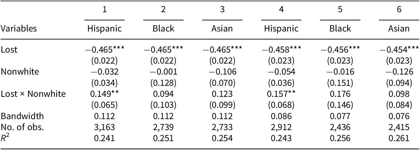
Table A2 replicates the main specification (Table 2) separately for Hispanic, Black, and Asian candidates relative to white candidates. Columns 1–3 use the same optimal bandwidth as the main analysis, while columns 4–6 use group-specific optimal bandwidths. The estimated persistence effects are positive and substantively similar across all groups, although statistical significance is observed only for Hispanic candidates, likely because of their larger sample size. The consistency in coefficient direction and magnitude suggests that the main finding is not driven by any single racial or ethnic subgroup.
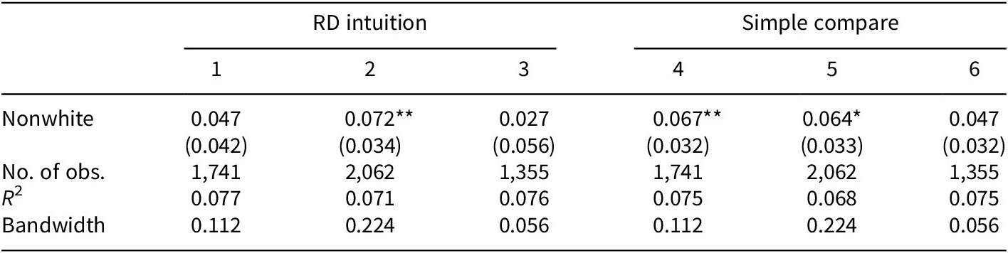
Additionally, California city council elections are typically staggered, with elections held every two years to fill a subset of seats. As a result, losing candidates may rerun before the next four-year cycle. To examine this possibility, I restrict the sample to losing candidates near the electoral threshold and analyze rerunning behavior within two years of defeat. Table A3 reports the results. Columns 1–3 estimate RD-style specifications that allow separate trends by race, while columns 4–6 report simpler models without trend controls.
Column 1 of Table A3, the preferred specification, uses the optimal bandwidth from the main analysis and allows for separate trends by race. It shows that losing nonwhite candidates are more likely to run again in two years than white candidates, although the estimate is not statistically significant. While statistical significance varies across bandwidth choices, the positive pattern is consistent across specifications. These findings reinforce the main results and suggest that the four-year estimates may understate racial differences in persistence because some nonwhite candidates rerun and win during the intermediate election cycle.
Consequences of persistence
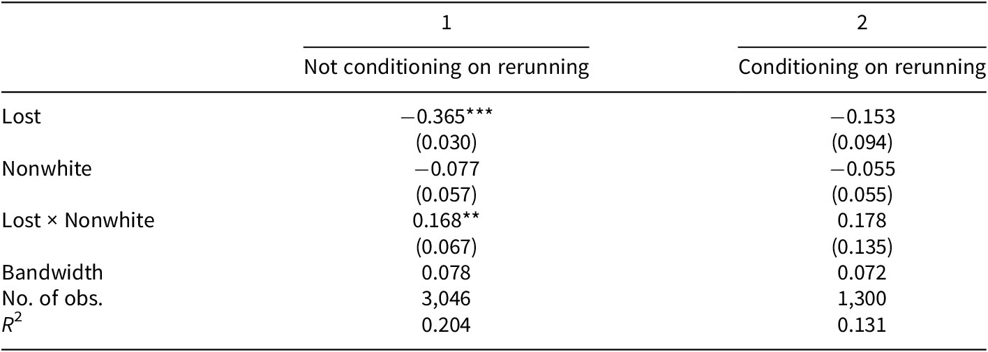
Will this resilience pay off? Table 3, which shows the winning probabilities in election year
$ t+4 $
 , provides insights. The two columns differ in how candidates who do not run again are coded. The outcome variable for the first specification is not conditional on rerunning, and the regression includes all marginal close election candidates. Candidates who do not rerun are coded as having lost the election, and their chance of winning in election year
$ t+4 $
 is set to 0. Column 2 shows the winning probability conditional on rerunning, where the candidates who do not rerun are excluded from the regression. This explains the difference in observations. The optimal bandwidths are selected separately for each analysis.
Effect of electoral outcome and race on subsequent electoral success

Table 3. Long description
The table presents regression coefficients for two models. Column 1 represents Not conditioning on rerunning, and Column 2 represents Conditioning on rerunning.
Row-by-row data:
* Lost: Model 1 is minus 0.365 with three asterisks (standard error 0.030); Model 2 is minus 0.153 (standard error 0.094).
* Nonwhite: Model 1 is minus 0.077 (standard error 0.057); Model 2 is minus 0.055 (standard error 0.055).
* Lost multiplied by Nonwhite: Model 1 is 0.168 with two asterisks (standard error 0.067); Model 2 is 0.178 (standard error 0.135).
* Bandwidth: Model 1 is 0.078; Model 2 is 0.072.
* Number of observations: Model 1 is 3,046; Model 2 is 1,300.
* R super 2: Model 1 is 0.204; Model 2 is 0.131.
Note: Significance levels are indicated as three asterisks for p < 0.01 and two asterisks for p < 0.05. Standard errors are in parentheses.
Note: The outcome variable is whether a candidate wins in the next election. Column 1 codes candidates who do not run again as a lose. Column 2 codes not rerunning candidates as missing values. Standard errors are clustered at the county level. County and year fixed effects are included in each specification. Significance levels are indicating as: ***p<0.01, **p<0.05, *p<0.1.
When not conditioning on rerunning, the coefficient of Lost × Nonwhite is significantly greater than zero, indicating that nonwhite candidates who lost in phase
$ t $
 are more likely to be elected in phase
$ t+4 $
 than their white peers. When conditioning on rerunning, the coefficient of Lost × Nonwhite is large enough to cancel out the negative effect on “lost,” albeit not significantly different from zero. This would suggest that conditional on rerunning, losing nonwhite candidates win at roughly the same rate as winning nonwhite candidates. In other words, these results indicate that electoral persistence can be rewarded.
Both results confirm that the higher rerunning probability or extra resilience of losing nonwhite candidates pays off by holding the same winning possibility in the following elections. Note that the results remain robust if we use the optimal bandwidth (11.2 percentage points) shown in Table 2. Therefore, the persistence of losing nonwhite candidates contributes to closing the racial representation gap.
Mechanisms
Theories of political trajectories posit that politicians decide whether to run or rerun for office by weighing the associated costs and benefits (Black Reference Black1972; Fox and Lawless Reference Fox and Lawless2004; Kiewiet and Zeng Reference Kiewiet and Zeng1993; Wasserman Reference Wasserman2018). In this framework, a candidate runs if the expected benefit of holding office, weighted by the probability of winning, exceeds the costs of running. Following Black (Reference Black1972), this can be expressed as
$ {P}^{\ast }B-C $
 , where P is the perceived probability of winning, B represents the benefits of office, and C captures the costs of running.
In the RDD, candidates near the cutoff are quasi-randomly assigned to win or lose, implying that their perceived probability of winning is locally similar. This allows the analysis to focus on the differences in B and C. Because these components are not directly observable, I use candidates’ occupational backgrounds as a proxy for differences in opportunity costs and perceived benefits of holding office.
Candidates from different occupational backgrounds may face different incentives for political persistence. Those from business careers are likely to incur higher opportunity costs due to foregone earnings. In contrast, candidates from community- or public-oriented roles may have stronger commitments to their communities, implying greater perceived nonmaterial benefits from holding office.
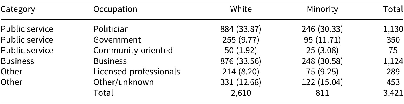
Table A4 presents a cross-tabulation of occupational categories by race. Occupations are coded from candidates’ ballot designations using keyword matching. I classify occupations into six groups: Politician, Government, Community-Oriented, Business, Licensed Professions, and Other/Unknown,Footnote 9 and further group them into three broader categories: Public Service (Politician, Government, Community-Oriented), Business, and Other. Minority candidates are more likely to come from non-elected public sector and community-oriented backgrounds, while white candidates are more concentrated in business occupations. Differences in the community-oriented category are statistically significant (
$ p=0.048 $
 ).
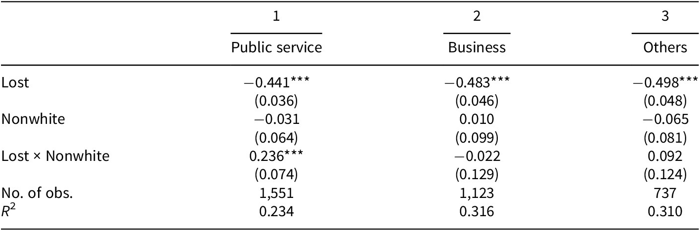
Table 4 examines whether the persistence effect varies across occupational backgrounds. The results show that the greater persistence of minority candidates is concentrated among candidates from public-service occupations. In contrast, the estimated effect for candidates from business occupations is negative, although statistically insignificant. Candidates in licensed professions and the residual Other/Unknown category also exhibit positive but statistically insignificant estimates.
Electoral persistence by occupation type

Table 4. Long description
The table consists of four columns. The first column lists variables, while columns 1, 2, and 3 represent Public service, Business, and Others respectively.
* Lost: Public service is -0.441 (standard error 0.036); Business is -0.483 (standard error 0.046); Others is -0.498 (standard error 0.048). All are significant at p < 0.01.
* Nonwhite: Public service is -0.031 (0.064); Business is 0.010 (0.099); Others is -0.065 (0.081).
* Lost multiplied by Nonwhite: Public service is 0.236 (0.074) significant at p < 0.01; Business is -0.022 (0.129); Others is 0.092 (0.124).
* Number of observations: Public service has 1,551; Business has 1,123; Others has 737.
* R super 2: Public service is 0.234; Business is 0.316; Others is 0.310.
Note: The outcome variable is whether a candidate runs again for office in four years. Standard errors are clustered at the county level.
Note. The outcome variable is whether a candidate runs again for office in four years. Standard errors are clustered at the county level. County and year fixed effects are included in each specification. Significance levels are indicating as: ***p<0.01, **p<0.05, *p<0.1.
Importantly, the greater persistence of minority candidates appears to be driven primarily by minority candidates from public-service backgrounds. As shown in Table A4, minority candidates are more likely than white candidates to come from government and community-oriented occupations. Taken together, these findings are consistent with a cost–benefit explanation of political persistence: candidates from public-service backgrounds may place greater value on the nonmaterial benefits of holding office or face lower opportunity costs of continued political participation. Consequently, the overrepresentation of minority candidates in these occupations may partially explain their greater persistence following an electoral defeat.
While occupational backgrounds may shape motivation by influencing the perceived benefits of holding office, differences in candidate capacity may also contribute to political persistence. Additional analyses examining candidate capacity are reported in Appendix B.
Conclusion
This article investigates racial differences in electoral reentry after a loss in local government elections. Empirical data from California city council elections and a close election RDD reveal that losing nonwhite candidates are more likely to rerun for office compared to losing white candidates. Conditional on rerunning, the probability of winning a subsequent election is similar across racial groups. Thus, the greater persistence of losing nonwhite candidates helps narrow the racial representation gap. The analysis also identifies a potential mechanism: minority candidates are more likely to come from public-service and community-oriented occupations, which may encourage continued political engagement after defeat.
This study contributes to the broader literature by addressing a key gap – the lack of causal research on racial differences in politicians’ electoral persistence. It provides one of the first causal examinations of racial differences in electoral persistence using detailed candidate-level electoral data. While these findings provide valuable insights, it is important to acknowledge the limitations and outline directions for future research. First, candidate-level information is limited, and many potentially relevant characteristics, such as campaign fundraising and educational background, are not consistently available. Future research could examine whether these factors help explain racial differences in electoral persistence as richer candidate-level data become available. Second, because this study focuses on California, caution should be exercised when generalizing the findings to other states with different political and demographic contexts. Finally, although no significant racial differences are observed in the electoral persistence of candidates who narrowly win office, disparities may exist in the pursuit of higher office, an outcome not examined in this study because of data limitations. Future research should examine whether similar patterns hold in elections for state legislatures, the US House of Representatives, and the US Senate.
Data availability statement
Replication materials are available on the SPPQ Dataverse at https://dataverse.harvard.edu/dataset.xhtml?persistentId=doi:10.7910/DVN/L7F1WN (Wang Reference Wang2026).
Acknowledgments
The author is grateful to Daniel B. Jones for his advice and support throughout this project.
Funding statement
The authors received no financial support for the research, authorship, and/or publication of this article.
Competing interests
The author declared no potential competing interests with respect to the research, authorship, and publication of this article.
Author biography
Xiaohong Wang is an Assistant Professor in the Department of Political Science and Criminal Justice at the University of South Alabama. Her research focuses on race and ethnicity, political representation, and criminal justice.
Appendix A: Tables and graphs
Linear regression discontinuity specification.

Figure A1. Long description
A two-panel figure with a shared x-axis labeled Margin vote share ranging from negative 0.2 to 0.2 and a y-axis labeled Probability of Running Again ranging from 0 to 1. Both panels feature a vertical dashed line at 0 representing the treatment threshold.
Left Panel: Titled All Candidates, Polynomial equals 1. To the left of 0, open circles are clustered between 0.1 and 0.4 with a flat linear regression line. To the right of 0, there is a significant upward jump, with circles clustered between 0.6 and 0.8 and a slightly positive linear slope.
Right Panel: Titled By Race, Polynomial equals 1. This panel disaggregates data into Minority (black circles) and White (gray diamonds).
* To the left of 0, both groups show low probabilities between 0 and 0.4 with relatively flat regression lines.
* To the right of 0, both groups show a sharp vertical jump. The White group (gray diamonds) shows a positive linear trend increasing from 0.6 to 0.8. The Minority group (black circles) shows a slightly negative linear trend starting near 0.7 and decreasing toward 0.6 as the margin increases.
A legend at the bottom right identifies black circles as Minority and gray diamonds as White.
Electoral outcome and subsequent participation by race

Table A1. Long description
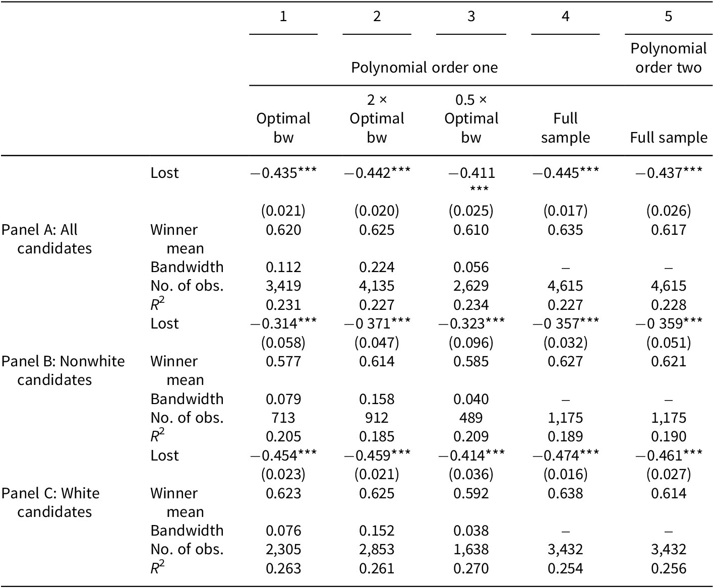
The table is organized into five columns representing different statistical specifications. Columns 1 through 4 use Polynomial order one with varying bandwidths (Optimal bw, 2 times Optimal bw, 0.5 times Optimal bw, and Full sample). Column 5 uses Polynomial order two with the Full sample. The table is divided into three vertical panels.
Panel A: All candidates
- Lost: Coefficients range from minus 0.411 to minus 0.445, all significant at p < 0.01.
- Winner mean: Ranges from 0.610 to 0.635.
- Number of observations: Ranges from 2,629 to 4,615.
- R super 2: Ranges from 0.227 to 0.234.
Panel B: Nonwhite candidates
- Lost: Coefficients range from minus 0.314 to minus 0.371, all significant at p < 0.01.
- Winner mean: Ranges from 0.577 to 0.627.
- Number of observations: Ranges from 489 to 1,175.
- R super 2: Ranges from 0.185 to 0.209.
Panel C: White candidates
- Lost: Coefficients range from minus 0.414 to minus 0.474, all significant at p < 0.01.
- Winner mean: Ranges from 0.592 to 0.638.
- Number of observations: Ranges from 1,638 to 3,432.
- R super 2: Ranges from 0.254 to 0.270.
Standard errors are provided in parentheses below each ‘Lost’ coefficient. The note indicates the outcome variable is whether a candidate runs again in four years, with standard errors clustered at the county level.
Note: The outcome variable is whether a candidate runs again for office in four years. Standard errors are clustered at the county level. County and year fixed effects are included in each specification. Significance levels are indicated as: ***p < 0.01, **p < 0.05, *p < 0.1.
Electoral outcome and subsequent participation: disaggregated by race

Table A2. Long description
The table consists of six columns. Columns 1 through 3 use a fixed bandwidth of 0.112, while columns 4 through 6 use group-specific bandwidths. The columns are paired by race: Hispanic (1 and 4), Black (2 and 5), and Asian (3 and 6).
* Lost: Values are -0.465 for columns 1, 2, and 3; -0.458 for column 4; -0.456 for column 5; and -0.454 for column 6. All are significant at p < 0.01.
* Nonwhite: Values range from -0.001 to -0.126, with standard errors in parentheses below each.
* Lost multiplied by Nonwhite: Column 1 is 0.149 (p < 0.05); Column 2 is 0.094; Column 3 is 0.123; Column 4 is 0.157 (p < 0.05); Column 5 is 0.176; Column 6 is 0.098.
* Bandwidth: 0.112 for columns 1-3; 0.086 for column 4; 0.077 for column 5; 0.076 for column 6.
* Number of observations: 3,163 (Col 1); 2,739 (Col 2); 2,733 (Col 3); 2,912 (Col 4); 2,436 (Col 5); 2,415 (Col 6).
* R super 2: Values range from 0.241 to 0.261.
Note: The outcome variable is whether a candidate runs again for office in four years. Each model compares Hispanic vs. white, Black vs. white, and Asian vs. white candidates. Columns 1–3 report results using the same optimal bandwidth as in the main analysis (0.112). Columns 4–6 report results using group-specific bandwidths. Standard errors are clustered at the county level. County and year fixed effects are included in all specifications. Significance levels are indicated as ***p<0.01, **p<0.05, *p<0.1.
Subsequent political participation within two years for losing candidates

Table A3. Long description
The table is organized into six columns. Columns 1 through 3 are grouped under R D intuition, and columns 4 through 6 are grouped under Simple compare.
Row 1: Nonwhite coefficients.
Column 1: 0.047 with a standard error of 0.042.
Column 2: 0.072 double asterisk with a standard error of 0.034.
Column 3: 0.027 with a standard error of 0.056.
Column 4: 0.067 double asterisk with a standard error of 0.032.
Column 5: 0.064 asterisk with a standard error of 0.033.
Column 6: 0.047 with a standard error of 0.032.
Row 2: Number of observations.
Columns 1 and 4: 1,741.
Columns 2 and 5: 2,062.
Columns 3 and 6: 1,355.
Row 3: R super 2 values.
Column 1: 0.077.
Column 2: 0.071.
Column 3: 0.076.
Column 4: 0.075.
Column 5: 0.068.
Column 6: 0.075.
Row 4: Bandwidth.
Columns 1 and 4: 0.112.
Columns 2 and 5: 0.224.
Columns 3 and 6: 0.056.
Note: Significance levels are indicated as double asterisk for p less than 0.05 and single asterisk for p less than 0.1.
Note: Outcome variable indicates whether a candidate runs again for office in two years. Columns 1–3 report results from specifications that allow for separate trends by including an interaction between minority status and vote margin, capturing the RD-style intuition. Columns 4–6 present simpler specifications without fitted trends. County and year fixed effects are included in all specifications. Significance levels are indicated as ***p<0.01, **p<0.05, *p<0.1.
Occupational background by race

Table A4. Long description
The table consists of five columns: Category, Occupation, White, Minority, and Total. Data for White and Minority columns include counts followed by percentages in parentheses.
* Public service category:
- Politician: White 884 (33.87), Minority 246 (30.33), Total 1,130.
- Government: White 255 (9.77), Minority 95 (11.71), Total 350.
- Community-oriented: White 50 (1.92), Minority 25 (3.08), Total 75.
* Business category:
- Business: White 876 (33.56), Minority 248 (30.58), Total 1,124.
* Other category:
- Licensed professionals: White 214 (8.20), Minority 75 (9.25), Total 289.
- Other/unknown: White 331 (12.68), Minority 122 (15.04), Total 453.
* Totals:
- The final row shows total counts: White 2,610, Minority 811, and a grand total of 3,421.
Not: Occupations are coded from candidates’ ballot designations at the time of candidacy using keyword matching. Entries report counts, with column percentages within each racial group reported in parentheses. “Category” groups occupations into broader classifications used in the analysis. “Licensed Professions” include education, legal, and medical occupations.
Appendix B: Capacity hypothesis
The capacity hypothesis is also grounded in the cost–benefit framework of political participation, but it primarily operates through the cost component. Prior research highlights the role of monetary resources in campaign capacity (Dolan and Shah Reference Dolan and Shah2020; Thomsen Reference Thomsen2025). To proxy for general and campaign capacity, I identify a group of occupations that require substantial education and professional training, such as doctors, attorneys, and professors. These occupations capture candidates’ general qualifications and potential access to resources. White candidates are somewhat more likely to be in these positions, but the differences are not statistically significant. This suggests that differences in campaign capacity are unlikely to be the primary driver of the observed persistence patterns documented in this article.
In addition to monetary costs, prior research also identifies differences in psychological costs of running for office, including harassment and threats faced by minority candidates (Collignon and Rüdig Reference Collignon and Rüdig2020; Tenove and Tworek Reference Tenove and Tworek2020). These factors are not directly observable in the current dataset. However, if such costs were the dominant factor shaping electoral persistence, minority candidates would be expected to be less likely to run again after a defeat. This prediction is inconsistent with the empirical findings, which show that minority candidates are more likely than white candidates to rerun following a narrow loss.




 Open access

