2.1. Satellite and reanalysis data

The dataset comprises 16 years (2003–2018) of cloud, aerosol, and meteorology data for the South-East Atlantic (SEA) low-level cloud region, which is impacted by smoke during the biomass burning season (30°W-15°E–25°S-0°, June–October).

The cloud observations are obtained from the Moderate Resolution Imaging Spectroradiometer (MODIS, Platnick et al., Reference Platnick, King and Hubanks2015) and the Clouds and the Earth’s Radiant Energy System (CERES, Doelling et al., Reference Doelling, Loeb, Keyes, Nordeen, Morstad, Nguyen, Wielicki, Young and Sun2013, Reference Doelling, Sun, Nguyen, Nordeen, Haney, Keyes and Mlynczak2016) instrument aboard the Aqua satellite. The meteorological variables are downloaded from the ERA5 (Hersbach et al., Reference Hersbach, Bell, Berrisford, Biavati, Horányi, Sabater, Nicolas, Peubey, Radu, Rozum, Schepers, Simmons, Soci, Dee and Thébaut2018a, Reference Hersbach, Bell, Berrisford, Biavati, Horányi, Sabater, Nicolas, Peubey, Radu, Rozum, Schepers, Simmons, Soci, Dee and Thébaut2018b) and CAMS reanalyses (Inness et al., Reference Inness, Ades, Agustí-Panareda, Barré, Benedictow, Blechschmidt, Dominguez, Engelen, Eskes, Flemming, Huijnen, Jones, Kipling, Massart, Parrington, Peuch, Razinger, Remy, Schulz and Suttie2019) from ECMWF. The products used in this study are: daytime cloud fraction (CF), cloud optical depth (COD), cloud droplet effective radius ( $ {r}_{\mathrm{eff}} $ ) and Aerosol Optical Depth (AOD) from the daily level 3 $ 1{}^{\circ}\times 1{}^{\circ} $ MODIS product; the reflected top-of-atmosphere (TOA) shortwave flux ( $ \mathrm{SW}\uparrow $ ) from the daily level 3 $ 1{}^{\circ}\times 1{}^{\circ} $ CERES product; pressure-level wind speeds and relative humidity from ERA5; pressure-level mixing ratios of BC and OC from CAMS. Using the adiabaticity assumption (Brenguier et al., Reference Brenguier, Pawlowska, Schüller, Preusker, Fischer and Fouquart2000; Quaas et al., Reference Quaas, Boucher and Lohmann2006), we derive the cloud depth $ H $ from COD and $ {r}_{\mathrm{eff}} $ . The key variables are listed in Table 1.

Table 1.

Causal graph node variables and their descriptions

Table 1. Long description

The table consists of two columns: Graph node and Description.

* B B A: Biomass burning aerosols. Total mass of B C and O C in the atmospheric column from C A M S, or M O D I S A O D to evaluate proxy confounding.

* r sub eff: Cloud droplet effective radius from M O D I S.

* H: Cloud depth, calculated from M O D I S retrievals using the adiabaticity assumption.

* C O D sub w: Cloud Optical Depth from M O D I S, weighted by the grid-box cloud fraction.

* S W up-arrow: Reflected top-of-atmosphere S W radiation flux from C E R E S.

* R H sub B L: Relative humidity from E R A 5, averaged over pressure levels below the boundary layer height.

* U sub 700: Eastward wind speed from E R A 5 at 700 hPa to capture mid-tropospheric transport by the Southern African Easterly Jet.

The data are co-located on the $ 1{}^{\circ}\times 1{}^{\circ} $ grid of the MODIS data using a conservative regridding approach (Zhuang et al., Reference Zhuang, Dussin, Huard, Bourgault, Banihirwe, Raynaud, Malevich, Schupfner, Filipe, Levang, Gauthier, Jüling, Almansi, Richard Scott, Rondeau, Rasp, Smith, Stacheleck, Plough, Pierre, Bell, Caneill and Li2023) and the reanalysis data are interpolated to the approximate local crossing time of the Aqua satellite. Among cloudy pixels, only low marine cloud pixels, identified as having a cloud top pressure larger than 680 hPa, are kept in the analysis.

2.2. Causal inference

The causal workflow includes four steps, summarized in Figure 2: (1) assumption of a groundtruth causal graph, (2) computation of partial sensitivities from observations, with control variables dictated by the graph, (3) computation of total and mediated effects from the partial sensitivities, and (4) comparison to other causal graphs and computation of resulting biases.

Figure 2.

Summary of the method, decomposed in 4 steps, from (1) assumption of the reference causal graph to (4) computation of biases in radiative effect estimates.

Figure 3 shows the “Reference graph,” describing the pathways by which BBAs affect the SW radiation budget of the SEA region (Step 1). Its structure is hypothesized from expert knowledge and is not obtained from data-driven techniques such as causal discovery (Runge et al., Reference Runge, Gerhardus, Varando, Eyring and Camps-Valls2023). Like in Figure 1, the colors of the arrow identifiers $ {a}_n $ highlight the direct (ARI), indirect (ACI, cloud-mediated), and semi-direct (adjustments to ARI, humidity-mediated) pathways through which BBAs modify SW radiation at TOA.

Figure 3.

Quantified causal links for the reference graph. Arrow colors correspond to the normalized magnitude of causal links between two variables, for contemporaneous effects (straight arrows) and lagged effects (curved arrows), while node colors correspond to the magnitude of autodependency links.

Causal effect estimation is done with the Python Tigramite package (https://github.com/jakobrunge/tigramite) following Wright’s linear path method (Wright, Reference Wright1921; Runge et al., Reference Runge, Petoukhov, Donges, Hlinka, Jajcay, Vejmelka, Hartman, Marwan, Paluš and Kurths2015). The estimation starts with the derivation of partial sensitivities, i.e., the values for each causal arrow in the graph, yielding the arrow colors in Figure 3 (Step 2). Once the causal links have been estimated, causal effects between two variables that are not directly linked by an arrow are calculated by tracing the path(s) that link the two variables and multiplying the coefficients along these paths (Step 3). This is formalized in Equation 2.1, which shows how the total shortwave radiative effect of BBAs is obtained with a linear multiplication of partial senstivities:

(2.1) $$ {\displaystyle \begin{array}{r}{\mathrm{RE}}_{\mathrm{BBA}\to \mathrm{SW}}=-\frac{\mathrm{dSW}\uparrow }{\mathrm{dBBA}}\times \Delta {\mathrm{BBA}}_{\mathrm{Forcing}},\mathrm{where}:\underset{\mathrm{Total}\ \mathrm{effect}}{\underbrace{\frac{\mathrm{dSW}\uparrow }{\mathrm{dBBA}}}}={\left.\frac{\mathrm{\partial SW}\uparrow }{\mathrm{\partial BBA}}\right|}_{\mathrm{direct}}+{\left.\frac{\mathrm{\partial SW}\uparrow }{\mathrm{\partial BBA}}\right|}_{\mathrm{indirect}}+{\left.\frac{\mathrm{\partial SW}\uparrow }{\mathrm{\partial BBA}}\right|}_{\mathrm{semi}-\mathrm{direct}}\\ {}=\frac{\mathrm{\partial SW}\uparrow }{\mathrm{\partial BBA}}+\frac{\mathrm{\partial SW}\uparrow }{\partial {\mathrm{COD}}_{\mathrm{w}}}\frac{\partial {\mathrm{COD}}_{\mathrm{W}}}{\mathrm{\partial BBA}}+\frac{\mathrm{\partial SW}\uparrow }{\partial {\mathrm{RH}}_{\mathrm{BL}}}\frac{\partial {\mathrm{RH}}_{\mathrm{BL}}}{\mathrm{\partial BBA}}={a}_1+{a}_2{a}_3{a}_4+\underset{\begin{array}{c}\mathrm{non}\hbox{-} \mathrm{cloud}\\ {}\mathrm{semi}\hbox{-} \mathrm{direct}\end{array}}{\underbrace{a_5{a}_6}}+\underset{\begin{array}{c}\mathrm{cloud}\hbox{-} \mathrm{mediated}\\ {}\mathrm{semi}\hbox{-} \mathrm{direct}\end{array}}{\underbrace{\left({a}_5{a}_7+{a}_5{a}_8\left({a}_9+{a}_{10}{a}_3\right)\right){a}_4}},\\ {}\mathrm{and}:\Delta {\mathrm{BBA}}_{\mathrm{Forcing}}=\overline{{\mathrm{BBA}}_{\begin{array}{c}25\%\mathrm{Smokiest}\\ {}\mathrm{days}\end{array}}}-\overline{{\mathrm{BBA}}_{\begin{array}{c}25\%\mathrm{Least}\\ {}\mathrm{smoky}\ \mathrm{days}\end{array}}}\hskip0.1em \left(\mathrm{see}\;\mathrm{Fig}.A.2\right)\end{array}} $$

To estimate the impact of the main sources of statistical biases (Step 4), we repeat Steps 1 to 3 for “degraded” variants of the graph, as described in Table 2 and Supplementary Figure A.1.

Table 2.

Description of the causal graph variants considered in this study

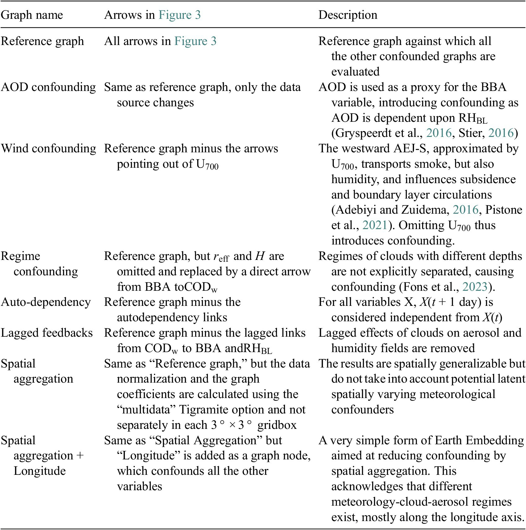
Table 2. Long description

The table consists of three columns: Graph name, Arrows in Figure 3, and Description.

* Reference graph: Includes all arrows in Figure 3. It serves as the baseline against which all other confounded graphs are evaluated.

* A O D confounding: Same arrows as the reference graph but uses A O D as a proxy for B B A, introducing confounding because A O D depends on R H sub B L.

* Wind confounding: Reference graph minus arrows pointing out of U sub 700. This omits the influence of the westward A E J - S on humidity, subsidence, and boundary layer circulations.

* Regime confounding: Reference graph but r sub eff and H are omitted and replaced by a direct arrow from B B A to C O D sub w. This fails to separate cloud depth regimes.

* Auto-dependency: Reference graph minus autodependency links. It assumes X at time t plus 1 day is independent from X at time t.

* Lagged feedbacks: Reference graph minus lagged links from C O D sub w to B B A and R H sub B L. This removes lagged effects of clouds on aerosol and humidity fields.

* Spatial aggregation: Same arrows as reference graph, but uses the multidata Tigramite option for normalization and coefficients instead of separate 3 degree by 3 degree gridboxes.

* Spatial aggregation plus Longitude: Same as Spatial Aggregation but adds Longitude as a graph node to reduce confounding by spatial aggregation across different meteorology-cloud-aerosol regimes.

2.3. Practical considerations: linearity, spatial aggregation, uncertainty intervals

It can be questioned whether smoke-cloud-radiation interactions are linear (e.g., see Doherty et al., Reference Doherty, Saide, Zuidema, Shinozuka, Ferrada, Gordon, Mallet, Meyer, Painemal, Howell, Freitag, Dobracki, Podolske, Burton, Ferrare, Howes, Nabat, Carmichael, da Silva, Pistone, Chang, Gao, Wood and Redemann2022). Lohmann and Feichter (Reference Lohmann and Feichter2001) found that linear additivity of the direct, indirect, and semi-direct radiative effects of BBAs was a valid assumption on a global scale. To test this with our regional data, we do a multiple linear regression of $ \mathrm{SW}\uparrow $ with respect to its parents’ variables in the reference graph, namely, BBA, $ {\mathrm{COD}}_{\mathrm{w}} $ , $ {\mathrm{RH}}_{\mathrm{BL}} $ _, and $ \mathrm{SW}\uparrow \left(t-1\right) $ . On average for the region, the parent variables explain 76% of the variability in the TOA SW. We thus consider the linear approximation to be reasonable.

Because aggregation over large regions can induce spurious statistical associations due to spatially covarying meteorological influences (Grandey and Stier, Reference Grandey and Stier2010), we do not carry out the causal effect estimation of the large SEA region at once, but rather in sub-domains (Loeb and Schuster, Reference Loeb and Schuster2008) of size $ 3{}^{\circ}\times 3{}^{\circ} $ , each containing 9 ( $ 1{}^{\circ}\times 1{}^{\circ} $ ) grid points. The data are normalized and de-seasonalized by removing the mean seasonal cycle and dividing by the standard deviation of the seasonal cycle in each sub-domain. This means that the structure of the causal graph is spatially generalizable over the SEA region, but the causal effects are not. With the “Spatial Aggregation” graph of Table 2, we bypass this spatial segmentation and pool all sub-domains using multidata causal inference to compute spatially uniform causal effects. “Spatial Aggregation + Longitude” is an attempt at correcting the resulting aggregation bias while retaining spatial generalization of the results.

The uncertainties for the radiative effect estimates are computed with standard error propagation of the 68.2% ( $ \pm {\sigma}_{\mathrm{dev}} $ ) bootstrap error intervals (with 100 bootstrap members) around the estimates of the causal links. Maps showing causal effects and radiative effects feature stippling where the effects are not statistically different from 0, i.e., where the confidence interval includes 0.

3.1. Causal graph validation

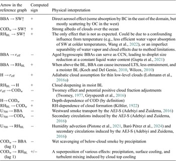
Figure 3 shows the computed values of every causal arrow featured in the reference causal graph (Step 2 in Figure 2). The causal links are resolved spatially on a $ 3{}^{\circ}\times 3{}^{\circ} $ grid (Supplementary Figure A3), but a domain-wide mean is shown here. The analysis of these values constitutes a physical validation of the method, as the signs of the effects correspond to the direction of the expected physical mechanisms (Table 3).

Table 3.

Physical interpretation of the reference graph’s causal links (Figure 3)

Table 3. Long description

The table consists of three columns: Arrow in the reference graph, Computed sign, and Physical interpretation.

* B B A points to S W up arrow: Computed sign is plus. Physical interpretation is direct aerosol effect (absorption by B C in the east, scattering by O C in the west).

* C O D sub w points to S W up arrow: Computed sign is plus. Physical interpretation is strong albedo of clouds over the ocean.

* R H sub B L points to S W up arrow: Computed sign is plus. Physical interpretation is a confounding influence from temperature or imperfect separability of water vapor and cloud effects.

* B B A points to r sub eff: Computed sign is minus. Physical interpretation is aged hygroscopic B B As serving as C C N, leading to droplet size reduction.

* B B A points to R H sub B L: Computed sign is plus. Physical interpretation is B B A causing increased L T S, less entrainment, and a moister B L.

* H points to r sub eff: Computed sign is plus. Physical interpretation is adiabatic cloud assumption for thin low-level clouds.

* R H sub B L points to H: Computed sign is plus. Physical interpretation is cloud deepening in moist B L.

* r sub eff points to C O D sub w: Computed sign is minus. Physical interpretation is Twomey effect and potential positive cloud fraction adjustments.

* H points to C O D sub w: Computed sign is minus. Physical interpretation is depth-dependence of C O D.

* R H sub B L points to C O D sub w: Computed sign is plus. Physical interpretation is R H-dependence of cloud formation.

* U sub 700 points to B B A: Computed sign is minus. Physical interpretation is westward smoke transport by the A E J-S.

* U sub 700 points to C O D sub w: Computed sign is minus. Physical interpretation is secondary circulations induced by the A E J-S.

* U sub 700 points to R H sub B L: Computed sign is minus. Physical interpretation is humidity advection and secondary circulations induced by the A E J-S.

* C O D sub w points to B B A (lag 1): Computed sign is minus. Physical interpretation is wet scavenging of below-cloud smoke by precipitation.

* C O D sub w points to R H sub B L (lag 1): Computed sign is plus or minus. Physical interpretation is a superposition of precipitation, surface cooling, and turbulent mixing.

3.2. Total shortwave effect of biomass burning aerosols

Figure 4 shows the total SW radiative effect of BBAs, as well as the fractions of that effect that are direct (non-mediated), indirect (cloud-mediated), and semi-direct ( $ {\mathrm{RH}}_{\mathrm{BL}} $ -mediated), as calculated using the path approach applied to the causal links computed just above (Step 3 in Figure 2). The smoke emitted over the SEA stratocumulus region during the biomass burning season causes a net regional cooling of $ \approx -2.5\;\mathrm{W}\;{\mathrm{m}}^{-2} $ . The direct, indirect, and semi-direct pathways contribute almost equally to this cooling.

Figure 4.

BBA radiative effect per pathway: (a) direct, (b) indirect, (c) semi-direct, and (d) resulting total (note the different color scale). The region-average BBA shortwave radiative effect is displayed in the upper left corner. Stippling indicates where the bootstrap confidence intervals include 0.

The warming/cooling dipole in total BBA radiative effect from east to west is mostly attributable to the direct radiative effect. This is due to the presence of dark-absorbing aerosols overlying a dense bright stratocumulus deck in the east, leading to a local warming of up to $ \approx 1\;\mathrm{W}\;{\mathrm{m}}^{-2} $ . In the west, cloud cover is sparser, and organic aerosols have photochemically “whitened” and become more efficient at scattering during atmospheric transport (e.g., Carter et al., Reference Carter, Heald, Cappa, Kroll, Campos, Coe, Cotterell, Davies, Farmer, Fox, Garofalo, Hu, Langridge, Ezra, Murphy, Pokhrel, Shen, Szpek, Taylor and Wu2021), leading to local cooling effects of more than $ -2\;{\mathrm{Wm}}^{-2} $ . Similar patterns have been found in reanalysis and model data, but model results are highly dependent on their choice of physical parameters and forcing methodologies (Myhre et al., Reference Myhre, Samset, Schulz, Balkanski, Bauer, Berntsen, Bian, Bellouin, Chin, Diehl, Easter, Feichter, Ghan, Hauglustaine, Iversen, Kinne, Kirkevåg, Lamarque, Lin, Liu, Lund, Luo, Ma, van Noije, Penner, Rasch, Ruiz, Seland, Skeie, Stier, Takemura, Tsigaridis, Wang, Wang, Xu, Yu, Yu, Yoon, Zhang, Zhang and Zhou2013; Zuidema et al., Reference Zuidema, Redemann, Haywood, Wood, Piketh, Hipondoka and Formenti2016; Mallet et al., Reference Mallet, Solmon, Nabat, Elguindi, Waquet, Bouniol, Sayer, Meyer, Roehrig, Michou, Zuidema, Flamant, Redemann and Formenti2020; Giuffrida et al., Reference Giuffrida, Johnson, Tatro, Zuidema and Gordon2025). Other observational studies (Kacenelenbogen et al., Reference Kacenelenbogen, Vaughan, Redemann, Young, Liu, Hu, Omar, LeBlanc, Shinozuka, Livingston, Zhang and Powell2019; Doherty et al., Reference Doherty, Saide, Zuidema, Shinozuka, Ferrada, Gordon, Mallet, Meyer, Painemal, Howell, Freitag, Dobracki, Podolske, Burton, Ferrare, Howes, Nabat, Carmichael, da Silva, Pistone, Chang, Gao, Wood and Redemann2022) have found stronger positive direct radiative effects of BBAs over the eastern SEA. However, the sampling of high-smoke events in these studies could have resulted in selection bias, whereas our estimates are representative of the whole duration of the biomass burning season in the SEA.

The indirect radiative effect is negative in the western part of the domain but slightly positive at the coast. In the west, this is due to aged and hygroscopic smoke being entrained into the boundary layer and acting as CCN (Gupta et al., Reference Gupta, McFarquhar, O’Brien, Delene, Poellot, Dobracki, Podolske, Redemann, LeBlanc, Segal-Rozenhaimer and Pistone2021), making clouds brighter and triggering cloud adjustments, like increased cloud cover and lifetime. In the east, freshly emitted BBAs are hydrophobic and cannot act as CCN (Redemann et al., Reference Redemann, Wood, Zuidema, Doherty, Luna, SE, Diamond, Shinozuka, Chang, Ueyama, Pfister, Ryoo, Dobracki, da Silva, Longo, Kacenelenbogen, Flynn, Pistone, Knox, Piketh, Haywood, Formenti, Mallet, Stier, Ackerman, Bauer, Fridlind, Carmichael, Saide, Ferrada, Howell, Freitag, Cairns, Holben, Knobelspiesse, Tanelli, Ecuyer, Dzambo, Sy, McFarquhar, Poellot, Gupta, O’Brien, Nenes, Kacarab, Wong, Small-Griswold, Thornhill, Noone, Podolske, Schmidt, Pilewskie, Chen, Cochrane, Sedlacek, Lang, Stith, Segal-Rozenhaimer, Ferrare, Burton, Hostetler, Diner, Seidel, Platnick, Myers, Meyer, Spangenberg, Maring and Gao2021). If hydrophobic smoke is entrained into the boundary layer, it competes with hydrophilic aerosols for water vapor, resulting in fewer and less bright cloud droplets (Ching et al., Reference Ching, Riemer and West2016). However, it is also possible that thick smoke layers overlying clouds bias the retrievals of cloud properties (Alfaro-Contreras et al., Reference Alfaro-Contreras, Zhang, Campbell, Holz and Reid2014). Modeling studies have also found negative indirect smoke radiative effects of the same magnitude, although some studies have a simplistic parameterization of aerosol-cloud interactions (Lohmann et al., Reference Lohmann, Feichter, Penner and Leaitch2000; Rap et al., Reference Rap, Scott, Spracklen, Bellouin, Forster, Carslaw, Schmidt and Mann2013; Giuffrida et al., Reference Giuffrida, Johnson, Tatro, Zuidema and Gordon2025).

While models have been shown to disagree on the sign and magnitude of the semi-direct effect (Sakaeda et al., Reference Sakaeda, Wood and Rasch2011; Allen et al., Reference Allen, Amiri-Farahani, Lamarque, Smith, Shindell, Hassan and Chung2019; Mallet et al., Reference Mallet, Solmon, Nabat, Elguindi, Waquet, Bouniol, Sayer, Meyer, Roehrig, Michou, Zuidema, Flamant, Redemann and Formenti2020), we detect uniform cooling, primarily driven by the cloud-mediated semi-direct effect (−0.7 W m⁻²) with a smaller contribution from the non-cloud semi-direct effect (−0.2 W m⁻²).

Our observational results highlight that the total smoke radiative effect results from almost equally cooling contributions of the direct, indirect, and semi-direct pathways. This finding can be used to constrain climate models that have previously found that the indirect effect dominates the total cooling (e.g., Lohmann and Feichter, Reference Lohmann and Feichter2001; Lu et al., Reference Lu, Liu, Zhang, Zhao, Meyer, Rajapakshe, Wu, Yang and Penner2018).

3.3. Sources of confounding

In Step 4 of the analysis, the reference graph is modified (Table 2) to single out sources of confounding bias (Figure 5).

Figure 5.

Biases in the smoke radiative effect caused by different sources of confounding.

Spatial aggregation results in the largest confounding bias with a −51% cooling bias compared to the reference graph. This is mostly due to the longitudinal gradient of meteorological regimes present in the SEA, with very bright clouds and a thick smoke layer in the east, but more dispersed clouds and less aerosols in the pristine western part of the domain, creating a spurious positive correlation among aerosols, cloud brightness, and reflected radiation. However, when simply adding longitude as a confounder node in the causal graph, the large bias almost vanishes (from −51% to +5%). This simple yet powerful change allows for spatial generalization while keeping bias at a minimum.

Diamond et al. (Reference Diamond, Dobracki, Freitag, Small-Griswold, Heikkila, Howell, Kacarab, Podolske, Saide and Wood2018) pointed out the time-dependence of smoke-cloud interactions over the SEA. Here, we detect that neglecting the auto-dependency of meteorological fields, and especially of $ {\mathrm{RH}}_{\mathrm{BL}} $ , $ {\mathrm{U}}_{700} $ and BBA (see node colors in Figure 3) leads to a 19% overestimation of the cooling influence of BBAs. It would be interesting to repeat the present analyses with a Lagrangian perspective to identify the exact processes responsible for this behavior.

Omitting $ {r}_{\mathrm{eff}} $ as a mediator of the indirect radiative effect of BBAs leads to an underestimation of the cooling influence of BBAs (by 14%). This is consistent with the findings of Fons et al. (Reference Fons, Runge, Neubauer and Lohmann2023) and is due to an overestimation of cloud optical depth decreases when aggregating data over different cloud regimes.

The AOD cooling bias (−11%) is due to the humidity-dependence of the AOD proxy, resulting in a spuriously enhanced correlation between RH and AOD (e.g., Gryspeerdt et al., Reference Gryspeerdt, Quaas and Bellouin2016; Stier, Reference Stier2016).

Neglecting confounding from large-scale winds leads to a small overestimation of the cooling influence of BBAs. This is coherent with Baró Pérez et al. (Reference Pérez, Diamond, Bender, Devasthale, Schwarz, Savre, Tonttila, Kokkola, Lee, Painemal and Ekman2024), who found a radiative bias due to moisture accompanying the smoke plume, although their cooling bias was much stronger than ours.

Importantly, while different sources of confounding might compensate each other to some degree, ignoring any of them would result in a loss of robustness as there is a lack of generalization power when confounding is present.