1 Introduction and background
In many flows, the molecular structure and state of the constituent fluid plays a significant role in the macroscopic behaviour of these flows. In such situations, some molecular modes of energy, especially those associated with longer time scales, may not be in thermal equilibrium – the flow is thus said to be in thermal non-equilibrium (TNE). This situation is encountered in low-temperature glow plasmas, flows behind shock waves and supersonic expansions and can be re-created in laboratories with lasers to excite specific molecular modes (Rich & Treanor Reference Rich and Treanor1970; Rich, Macheret & Adamovich Reference Rich, Macheret and Adamovich1996). TNE has also a significant effect on reaction rates in reacting flows and heat transfer characteristics in hypersonic vehicles. Although the asymptotic behaviour of simple steady laminar flows in TNE has been studied before (Vincenti & Kruger Reference Vincenti and Kruger1975), very few studies have focused on the interaction of turbulent fluctuations with TNE. These numerical (Liao, Peng & Luo Reference Liao, Peng and Luo2010) and experimental (Fuller et al. Reference Fuller, Hsu, Sanchez-Gonzalez, Dean, North and Bowersox2014) studies, nonetheless, show strong coupling between them. However, no general or systematic study is available to determine, for example, how the distribution of energy in different modes is affected by turbulence and how this depends on turbulence statistics as well as molecular properties. This is the thrust for the present study. Our objective here is to determine general statistical features of energy modes, in particular molecular vibration of diatomic molecules, when the flow is turbulent and in TNE. We show that, owing to the nonlinear nature of partially excited vibrational modes, turbulent fluctuations create statistically steady states that, unlike laminar flows, do not approach thermal equilibrium at long times. This has implications on the distribution of energy in different modes, namely, vibrational, translational and rotational molecular modes.
From quantum mechanics, the vibrational energy per unit mass for harmonic oscillators in thermodynamic equilibrium with translational temperature
 $T$
is given by
 $$\begin{eqnarray}\displaystyle e_{v}^{\ast }=\frac{R{\it\theta}_{v}}{\exp ({\it\theta}_{v}/T)-1}, & & \displaystyle\end{eqnarray}$$
where
 ${\it\theta}_{v}$
is the characteristic vibrational temperature,
 $R$
is the gas constant and an asterisk denotes thermal equilibrium. The translational and rotational energies, given by
 $e_{t}^{\ast }=(3/2)RT$
and
 $e_{r}^{\ast }=RT$
respectively, will be assumed to be in thermal equilibrium, which is justified given the relatively small number of collisions needed for equilibration (Hirschfelder, Curtiss & Bird Reference Hirschfelder, Curtiss and Bird1954). The combination of translational and rotational energies will be denoted by
 $e=e_{t}^{\ast }+e_{r}^{\ast }=(5/2)RT$
, where the asterisk is dropped in
 $e$
for simplicity in notation. Note that, while we are assuming diatomic molecules, the conclusions below are readily applicable to other molecular systems through the different numerical values of constants and prefactors.
In turbulent flows, hydrodynamics as well as thermodynamic variables experience fluctuations over a wide range of scales and it is useful to split a variable
 $f$
into mean and fluctuations, that is,
 $f=\overline{f}+f^{\prime }$
, where an overbar is a suitably defined average and clearly
 $\overline{f^{\prime }}=0$
. For simplicity in notation we will denote normalized fluctuations as
 $f^{\dagger }\equiv f^{\prime }/\overline{f}$
.
Two relevant parameters for compressible turbulence are the Taylor Reynolds number
 $R_{{\it\lambda}}=\sqrt{\overline{u^{\prime 2}}}{\it\lambda}\overline{{\it\rho}}/{\it\mu}$
(where
 ${\it\lambda}$
is the Taylor microscale,
 $\overline{{\it\rho}}$
the mean density and
 ${\it\mu}$
the mean viscosity) and the turbulent Mach number
 $M_{t}=\sqrt{3}\sqrt{\overline{u^{\prime 2}}}/c$
(where
 $c$
is the mean speed of sound). As detailed below, we present results at
 $R_{{\it\lambda}}\approx 38$
, 60 and 100 and turbulent Mach numbers between
 $M_{t}\approx 0.1$
and 0.8.
2 Direct numerical simulations
The analytical results presented below are compared to direct numerical simulations (DNS) of turbulence in a three-dimensional periodic domain governed by the Navier–Stokes equations. The fully compressible set of equations are solved with tenth-order compact schemes in space, and third-order low-storage Runge–Kutta in time. Molecular transport properties (viscosity and thermal diffusivity) follow power laws with temperature with an exponent of 0.5. Numerical details of the simulations including resolution studies and its implementation on massively parallel systems are included in Jagannathan & Donzis (Reference Jagannathan and Donzis2016). An important aspect of the present simulations, though, is the way in which energy is introduced in the system to generate turbulent fluctuations. A stationary state is maintained by stochastic forcing at the largest scales using solenoidal and dilatational modes (SF and DF for short) in the momentum equations (Donzis & Jagannathan Reference Donzis and Jagannathan2013). We also apply a combination of SF with stochastic forcing in the internal energy equation (EF for short), which can represent, for example, distributed exothermic reactions, and that leads to stronger fluctuations in temperature. The general forcing term is given by
 $$\begin{eqnarray}\displaystyle \boldsymbol{f}(\boldsymbol{x})=\mathop{\sum }_{|\boldsymbol{k}|<k_{F}}[s\,\hat{\boldsymbol{f}}_{\bot }(\boldsymbol{k})+(1-s)\hat{\boldsymbol{f}}_{\Vert }(\boldsymbol{k})]\text{e}^{-\text{i}\boldsymbol{k}\boldsymbol{\cdot }\boldsymbol{x}}, & & \displaystyle\end{eqnarray}$$
where
 $\hat{\boldsymbol{f}}_{\bot }(\boldsymbol{k})$
and
 $\hat{\boldsymbol{f}}_{\Vert }(\boldsymbol{k})$
are Fourier modes normal and parallel to the wavenumber vector constructed from integrated Ornstein–Uhlenbeck random processes with finite-time correlation. Forced wavenumbers are within a sphere of radius
 $k_{F}$
typically around 2. Purely solenoidal forcing (SF) is obtained with
 $s=1$
; purely dilatational forcing (DF) is obtained with
 $s=0$
. The reason for using multiple forcing schemes is to assess universal aspects of the flow as well as to reach regimes difficult to access otherwise such as those with very strong temperature fluctuations enabled by EF.
To maintain a statistically steady state, energy is removed from the system uniformly so that the mean temperature is kept constant as in Donzis & Jagannathan (Reference Donzis and Jagannathan2013). Consistent with results in the literature (e.g. Wang et al. Reference Wang, Wang, Xiao, Shi and Chen2010), our simulations show that results are insensitive of the details of the energy removal mechanism (Jagannathan & Donzis Reference Jagannathan and Donzis2016).
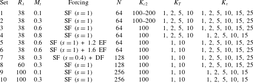
In order to assess scaling with different parameters, a very large DNS database has been generated and analysed. A summary of the parameter space and conditions covered by the simulations is shown in table 1.
Summary of parameters for all the simulations spanning wide regions of the parameter space: Reynolds number
 $R_{{\it\lambda}}$
.

Before proceeding further, we note that the analytical results below are derived in terms of temperature variance and temperature–density correlations. Depending on the type of forcing, these can be related to other parameters. For example, for SF we have (Donzis & Jagannathan Reference Donzis and Jagannathan2013)
 $$\begin{eqnarray}\displaystyle \left.\begin{array}{@{}c@{}}\overline{{T^{\dagger }}^{2}}\approx A^{2}({\it\gamma}-1)^{2}M_{t}^{4}/9,\\ \overline{{{\it\rho}^{\dagger }}^{2}}\approx A^{2}M_{t}^{4}/9,\\ \overline{{\it\rho}^{\dagger }T^{\dagger }}\approx A^{2}({\it\gamma}-1)M_{t}^{4}/9,\end{array}\right\} & & \displaystyle\end{eqnarray}$$
where
 ${\it\gamma}$
is the ratio of specific heats and
 $A$
is a flow-dependent constant. When DF is applied, however, these relations are not valid but still fluctuations are found to be accurately described as isentropic or more generally as polytropic. Then (Donzis & Jagannathan Reference Donzis and Jagannathan2013)
 $$\begin{eqnarray}\displaystyle \left.\begin{array}{@{}c@{}}\overline{{{\it\rho}^{\dagger }}^{2}}=\overline{{T^{\dagger }}^{2}}/({\it\gamma}-1)^{2},\\ \overline{{\it\rho}^{\dagger }T^{\dagger }}=\overline{{T^{\dagger }}^{2}}/({\it\gamma}-1).\end{array}\right\} & & \displaystyle\end{eqnarray}$$
(In what follows
 ${\it\gamma}$
is understood as a polytropic exponent, with the isentropic case being a particular instance.) Finally, when the energy equation is forced (i.e. EF), temperature and density fluctuations become more uncorrelated and it is not possible to identify a single parameter to represent their fluctuations.
3 Turbulence in thermal equilibrium
Consider first the case of a turbulent flow where vibrational energy is in complete thermal equilibrium, that is
 $e_{v}=e_{v}^{\ast }$
everywhere and at all times, with
 $e_{v}^{\ast }$
given by (1.1). Owing to temperature fluctuations, we clearly have
 $\overline{e_{v}^{\ast }}\neq e_{v}^{\ast }(\overline{T})$
where
 $e_{v}^{\ast }(\overline{T})$
is (1.1) evaluated at
 $T=\overline{T}$
. To see this, consider fluctuations around
 $e_{v}^{\ast }(\overline{T})$
. A Taylor expansion results in
 $e_{v}^{\ast }=e_{v}^{\ast }(\overline{T})+(\partial _{T}e_{v}^{\ast })T^{\prime }+(\partial _{T}^{2}e_{v}^{\ast })T^{\prime 2}/2+\cdots \,$
, where
 $\partial _{T}$
and
 $\partial _{T}^{2}$
represent first and second derivatives with respect to
 $T$
. These derivatives are always evaluated at
 $T=\overline{T}$
, which will not be explicitly indicated in equations for brevity. After averaging, we obtain
 $\overline{e_{v}^{\ast }}=e_{v}^{\ast }(\overline{T})+(\partial _{T}^{2}e_{v}^{\ast })\overline{T^{\prime 2}}/2+\cdots \,,$
which when combined with (1.1), can be rewritten as
 $$\begin{eqnarray}\displaystyle \frac{\overline{e_{v}^{\ast }}-e_{v}^{\ast }(\overline{T})}{e_{v}^{\ast }(\overline{T})} & = & \displaystyle g_{T}\overline{{T^{\dagger }}^{2}}\end{eqnarray}$$
 $$\begin{eqnarray}\displaystyle & {\approx} & \displaystyle A^{2}g_{M}M_{t}^{4},\end{eqnarray}$$
 $$\begin{eqnarray}\displaystyle g_{T}=K_{T}{\it\beta}((K_{T}-2){\it\beta}+K_{T}+2)({\it\beta}-1)^{-2}/2 & & \displaystyle\end{eqnarray}$$
and
 $$\begin{eqnarray}\displaystyle g_{M}=g_{T}({\it\gamma}-1)^{2}/9 & & \displaystyle\end{eqnarray}$$
depend only on the mean temperature and the molecular system through the non-dimensional parameter
 $$\begin{eqnarray}\displaystyle K_{T}\equiv {\it\theta}_{v}/\overline{T}, & & \displaystyle\end{eqnarray}$$
which compares the characteristic vibrational temperature to the mean translational temperature of the flow. From (1.1), we see that the equilibrium vibrational energy is a monotonically decreasing function of
 $K_{T}$
. For convenience we define
 ${\it\beta}\equiv e^{K_{T}}$
.
The last approximation (3.2) is obtained using (2.2), which is valid only for SF. The expression in terms of
 $\overline{{T^{\dagger }}^{2}}$
, however, is general and applicable to any flow with temperature fluctuations. This expression states that the average vibrational energy per unit mass departs from the value obtained in a non-fluctuating flow (with respect to the specific average chosen) at the same mean temperature. This is in contrast to the translational–rotational energy
 $e=(5/2)RT$
, which yields
 $\overline{e}=e(\overline{T})$
even in turbulent flows. A similar result is obtained for vibration if this mode is fully excited (
 ${\it\theta}_{v}/T\ll 1$
), in which case
 $e_{v}^{\ast }\approx RT$
. As we show below, this limiting case has significance not only in mean values but also in the symmetry of the probability density function of vibrational energy.
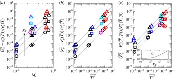
Effect of temperature fluctuations on mean vibrational energy in thermal equilibrium per unit mass (a,b) and per unit volume (c). Circles, squares and triangles correspond to
 $K_{T}=2$
, 5 and 10, respectively. Black, magenta, red and cyan are for SF, DF, SF + EF and DF + EF, respectively. Blue symbols are at
 $R_{{\it\lambda}}\approx 100$
with SF (sets 9 and 10). For the present simulations
 $A=1.2$
and
 ${\it\gamma}=1.4$
.

In figure 1(a,b) we compare (3.1) and (3.2) with DNS data, where averages are taken over space as typically done in isotropic simulations (Ishihara, Gotoh & Kaneda Reference Ishihara, Gotoh and Kaneda2009). In figure 1(a) we see very good agreement except for DF and EF cases, which is not unexpected since the relation used between temperature fluctuations and
 $M_{t}$
is only valid for SF. All cases collapse when data are cast in terms of temperature fluctuations (figure 1
b). The general expression in terms of
 $\overline{{T^{\dagger }}^{2}}$
holds independently of the physical mechanism responsible for these temperature fluctuations. We also note that, while the Mach-number dependence is strong, Reynolds-number effects are very weak. This is not unexpected since temperature fluctuations are known to be strongly affected by
 $M_{t}$
but only weakly affected by
 $R_{{\it\lambda}}$
(Donzis & Jagannathan Reference Donzis and Jagannathan2013).
A similar development can be done for the vibrational energy per unit volume
 $E_{v}^{\ast }\equiv {\it\rho}e_{v}^{\ast }$
. The relevance of this quantity can be seen readily in the context of our simulations, where the average is essentially an integration over the volume (divided by a constant), that is, the total vibrational energy in the domain. When (1.1) is multiplied by
 ${\it\rho}$
, the Taylor expansion now involves fluctuations in both temperature and density. Again, using (1.1) and averaging, we can rearrange the final expression, which, to leading order, is
 $$\begin{eqnarray}\displaystyle \frac{\overline{E_{v}^{\ast }}-E_{v}^{\ast }(\overline{T},\overline{{\it\rho}})}{E_{v}^{\ast }(\overline{T},\overline{{\it\rho}})} & = & \displaystyle g_{T}\overline{{T^{\dagger }}^{2}}+g_{{\it\rho}T}\overline{{\it\rho}^{\dagger }T^{\dagger }}\end{eqnarray}$$
 $$\begin{eqnarray}\displaystyle & {\approx} & \displaystyle G_{T}\overline{{T^{\dagger }}^{2}}\end{eqnarray}$$
 $$\begin{eqnarray}\displaystyle & {\approx} & \displaystyle A^{2}G_{M}M_{t}^{4},\end{eqnarray}$$
 $$\begin{eqnarray}\displaystyle G_{T}=g_{T}+g_{{\it\rho}T}/({\it\gamma}-1),\quad G_{M}=[g_{T}({\it\gamma}-1)+g_{{\it\rho}T}]({\it\gamma}-1)/9, & & \displaystyle\end{eqnarray}$$
with
 $$\begin{eqnarray}\displaystyle g_{{\it\rho}T}=K_{T}{\it\beta}/({\it\beta}-1). & & \displaystyle\end{eqnarray}$$
As before, (3.7) is valid for SF and DF, (3.8) is valid for SF, and (3.6) is the most general expression valid for all types of forcing.
An interesting observation emerges from a comparison between (3.6) and (1.1), which reveals that, unlike
 $e_{v}^{\ast }$
, the departures of
 $E_{v}^{\ast }$
from its non-fluctuating counterpart depend on the dynamics of turbulence. This is so because (1.1) as well as the first term in (3.6) depend only on the variance of temperature regardless of the mechanism generating those fluctuations. However, (3.6) depends also on the correlation between temperature and density, which is determined by the dynamics of thermodynamic variables in a particular flow.
The good agreement between (3.7) and the DNS with SF and DF forcings is shown in figure 1(c). It is readily verified that at low and high values of
 $K_{T}$
the dominant contribution comes from the
 $g_{{\it\rho}T}$
and
 $g_{T}$
terms, respectively. Thus, it is also seen that the EF cases, which are dominated by temperature fluctuations, also become a better approximation at high
 $K_{T}$
as the magnitude of
 $g_{{\it\rho}T}$
becomes relatively small.
An interesting consequence of (3.7) is that, since
 $G_{T}$
is always positive, then
 $\overline{E_{v}^{\ast }}>E_{v}^{\ast }(\overline{T})$
. This means that the total energy in the vibrational mode will always be larger when fluctuations of thermodynamic variables are present, even if the flow is in complete thermal equilibrium. Alternatively, this implies that, in order to maintain the same mean temperature (translational–rotational energy), a turbulent flow will store more energy in the vibrational mode than its non-fluctuating (laminar) counterpart. This result is a consequence of the specific nonlinear dependence of the equilibrium vibrational energy with temperature (1.1) when this mode is partially excited.
While these departures from a non-fluctuating flow increase with
 $K_{T}$
(inset of figure 1
c), the contribution from vibrational modes to the total energy decreases. Note, however, that the function
 $G_{T}$
asymptotes to
 $({\it\gamma}-1)^{-1}$
at high temperatures (low
 $K_{T}$
), and thus the relative difference approaches
 $({\it\gamma}-1)^{-1}\overline{{T^{\dagger }}^{2}}$
.
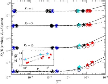
Ratio of average equilibrium vibrational and translational–rotational energy. Dashed lines (3.13) and open circles (DNS) are for
 $\overline{E_{v}^{\ast }}/\overline{E}$
. Solid lines (4.10) and closed stars (DNS with
 $K_{{\it\tau}}=10$
) are for
 $\overline{E_{v}}/\overline{E}$
. From top to bottom,
 $K_{T}=1$
, 5, 10 and 15, respectively. Different colours as in figure 1. Inset: variation of
 $\overline{E_{v}}/\overline{E_{v}^{\ast }}$
with
 $K_{{\it\tau}}$
for fixed
 $\overline{{T^{\dagger }}^{2}}\approx 10^{-2}$
and
 $K_{T}=10$
.

We now turn to the relative contribution of vibrational to translational–rotational energy. For laminar flows in thermal equilibrium, this is well known:
 $$\begin{eqnarray}\displaystyle \frac{E_{v}^{\ast }(\overline{T},\overline{{\it\rho}})}{E(\overline{T},\overline{{\it\rho}})}=\frac{2K_{T}}{5({\it\beta}-1)}. & & \displaystyle\end{eqnarray}$$
Because of the different effect of fluctuations of thermodynamic variables on different energy modes, we expect the distribution of energy to depend on these fluctuations. For example, the ratio of the average vibrational to translational–rotational energy, both in thermodynamic equilibrium, can be written, using (3.6) and
 $\overline{E}=E(\overline{T},\overline{{\it\rho}})(1+\overline{{\it\rho}^{\dagger }T^{\dagger }})$
(which results from decomposing
 $E={\it\rho}(5/2)RT$
into mean and fluctuations), as
 $$\begin{eqnarray}\displaystyle \frac{\overline{E_{v}^{\ast }}}{\overline{E}} & {\approx} & \displaystyle \frac{E_{v}^{\ast }(\overline{T},\overline{{\it\rho}})}{E(\overline{T},\overline{{\it\rho}})}\frac{1+g_{T}\overline{{T^{\dagger }}^{2}}+g_{{\it\rho}T}\overline{{\it\rho}^{\dagger }T^{\dagger }}}{1+\overline{{\it\rho}^{\dagger }T^{\dagger }}}\end{eqnarray}$$
 $$\begin{eqnarray}\displaystyle & {\approx} & \displaystyle \frac{E_{v}^{\ast }(\overline{T},\overline{{\it\rho}})}{E(\overline{T},\overline{{\it\rho}})}\frac{1+G_{T}\overline{{T^{\dagger }}^{2}}}{1+\overline{{T^{\dagger }}^{2}}/({\it\gamma}-1)},\end{eqnarray}$$
 $$\begin{eqnarray}\displaystyle r_{v}^{\ast }\equiv \frac{\overline{E_{v}^{\ast }}/\overline{E}}{E_{v}^{\ast }(\overline{T},\overline{{\it\rho}})/E(\overline{T},\overline{{\it\rho}})}, & & \displaystyle\end{eqnarray}$$
which measures the effect of turbulence on the distribution of energy across vibrational and translational–rotational modes. It is readily shown from (3.13) that
 $r_{v}^{\ast }$
tends to 1 and
 $({\it\gamma}-1)G_{T}$
for low and high levels of temperature fluctuations
 $\overline{{T^{\dagger }}^{2}}$
(or
 $M_{t}$
), respectively. However, the expansion in the numerator of (3.13) contains only the leading-order term. Higher-order terms will become important at, for example, higher
 $M_{t}$
where thermodynamic fluctuations may follow a log-normal distribution (Blaisdell, Mansour & Reynolds Reference Blaisdell, Mansour and Reynolds1993; Donzis & Jagannathan Reference Donzis and Jagannathan2013). In any case, we can see that, as
 $M_{t}$
increases, a larger fraction of the available energy will be stored in vibrational modes when the mean temperature of the flow is kept constant. Even if higher-order terms are included,
 $r_{v}^{\ast }$
may still plateau at intermediate Mach numbers since the denominator is a second-order polynomial without any approximation.
In summary, (3.13) shows that the distribution of energy among modes, even when complete thermal equilibrium is achieved instantaneously, will depend on the level of turbulent temperature fluctuations.
4 Turbulence in thermal non-equilibrium
We now turn to the situation where thermal equilibrium is not achieved instantaneously, that is, TNE. This is known to be the case, for example, in the laminar flow behind a strong shock where translational and rotational energy quickly reach equilibrium but vibration, associated with much larger time scales (Rich & Treanor Reference Rich and Treanor1970), attains equilibrium only after a relatively long period of time. This relaxation process can also be studied in molecular simulations (Liao et al. Reference Liao, Peng and Luo2010; Paul et al. Reference Paul, Kohale, Pratihar, Sun, North and Hase2014) as well as experiments (Fuller et al. Reference Fuller, Hsu, Sanchez-Gonzalez, Dean, North and Bowersox2014).
If the diatomic molecules are treated as harmonic oscillators, then the evolution of the vibrational energy of a fluid element convected by a macroscopic velocity field
 $\boldsymbol{u}$
can be written as (Hirschfelder et al.
Reference Hirschfelder, Curtiss and Bird1954)
 $$\begin{eqnarray}\displaystyle \frac{\partial {\it\rho}e_{v}}{\partial t}+\boldsymbol{{\rm\nabla}}\boldsymbol{\cdot }({\it\rho}e_{v}\boldsymbol{u})=\boldsymbol{{\rm\nabla}}\boldsymbol{\cdot }(D\boldsymbol{{\rm\nabla}}e_{v})+{\it\rho}\frac{e_{v}^{\ast }-e_{v}}{{\it\tau}_{v}}, & & \displaystyle\end{eqnarray}$$
where
 $\boldsymbol{u}$
is the advecting velocity field and
 $D$
is the diffusion coefficient, which is taken to be the same as that for translational energy, as a base case. While (4.1) assumes a Fickian process the analysis below leads to similar conclusions for any other model that can be written in conservative form as a divergence. This is so because our interest is in averaged quantities, which for statistically homogeneous flows results in vanishing transport terms. The last term in (4.1) represents the exchange mechanism between vibrational and translational modes according to the widely used Landau–Teller relaxation (Landau & Teller Reference Landau and Teller1936) with
 ${\it\tau}_{v}$
being the characteristic relaxation time, which can also be computed from theoretical considerations as
 ${\it\tau}_{v}=(c_{1}^{{\it\tau}_{v}}/p)\exp (c_{2}^{{\it\tau}_{v}}/T)^{1/3}$
where
 $c_{1}^{{\it\tau}_{v}}$
and
 $c_{2}^{{\it\tau}_{v}}$
are constants that depend on the molecular system (Hirschfelder et al.
Reference Hirschfelder, Curtiss and Bird1954). As in past studies (e.g. Olejniczak & Candler Reference Olejniczak and Candler1995; Bertolotti Reference Bertolotti1998), (4.1) is solved along with the compressible Navier–Stokes equations.
The last term in (4.1) acts as a restoring force for vibrational energy towards thermal equilibrium. In the absence of an advective velocity and diffusive effects,
 $E_{v}\equiv {\it\rho}e_{v}$
will relax exponentially towards
 $E_{v}^{\ast }$
, if the latter is constant, as in the case of a large bath. In a turbulent flow, however,
 $T$
experiences strong fluctuations in space and time, and therefore so does
 $E_{v}^{\ast }$
. The instantaneous
 $E_{v}$
will try to relax towards the fluctuating
 $E_{v}^{\ast }$
but will, in general, present some lag. Indeed, the departures from equilibrium will depend on how fast the relaxation process occurs compared to the fluctuations in
 $T$
.
Consider the following simple model. Cast (4.1) in a Lagrangian frame with
 $E_{v}^{\ast }=C(1+{\it\sigma}\sin ({\it\omega}t))$
, where
 $C$
is the mean equilibrium energy,
 ${\it\sigma}$
the amplitude of the fluctuations (in the real case it would be proportional to
 $\overline{{T^{\dagger }}^{2}}$
) and
 ${\it\omega}$
the frequency of the oscillations. If diffusion is neglected, the equation reads
 $\text{d}E_{v}/\text{d}t=(E_{v}^{\ast }-E_{v})/{\it\tau}_{v}$
. Furthermore, if for simplicity
 ${\it\tau}_{v}$
is assumed constant, it is easy to show that the steady-state solution will present a persistent departure from the equilibrium condition and in general
 $E_{v}\neq E_{v}^{\ast }$
. Indeed, the mean square of the departure is
 $$\begin{eqnarray}\displaystyle \frac{\overline{(E_{v}-E_{v}^{\ast })^{2}}}{\overline{E_{v}^{\ast }}^{2}}=\frac{({\it\tau}_{v}{\it\omega})^{2}}{1+({\it\tau}_{v}{\it\omega})^{2}}, & & \displaystyle\end{eqnarray}$$
with averages taken in time. Clearly, for slow perturbations relative to relaxation processes,
 ${\it\tau}_{v}{\it\omega}\ll 1$
, the departures vanish. For very rapid perturbations, departures increase but approach an asymptote at
 ${\it\tau}_{v}{\it\omega}\gg 1$
.
Turbulent flows possess a wide range of time scales. The most rapid fluctuations in a turbulent flow are associated with the so-called Kolmogorov time scale (Kolmogorov Reference Kolmogorov1941)
 ${\it\tau}_{{\it\eta}}\equiv ({\it\nu}/\langle {\it\epsilon}\rangle )^{1/2}$
, where
 ${\it\nu}$
is the mean kinematic viscosity and
 $\langle {\it\epsilon}\rangle$
the mean energy dissipation rate. Since the Prandtl number in the simulations is of order one, the smallest scales for the temperature field are expected to operate at a time scale comparable to
 ${\it\tau}_{{\it\eta}}$
(Monin & Yaglom Reference Monin and Yaglom1975). Thus, an important non-dimensional parameter to characterize the relaxation process in turbulent flows is the ratio
 $$\begin{eqnarray}\displaystyle K_{{\it\tau}}\equiv {\it\tau}_{v}/{\it\tau}_{{\it\eta}} & & \displaystyle\end{eqnarray}$$
(equivalent to
 ${\it\tau}_{v}{\it\omega}$
in the simple model above). To obtain a specific value
 $K_{{\it\tau}}$
in our simulations, we adjust the constant
 $c_{1}^{{\it\tau}_{v}}$
. The value of
 $c_{2}^{{\it\tau}_{v}}$
is taken to be approximately two orders of magnitudes larger than
 $\overline{T}$
(that is,
 $K_{c2}\equiv c_{2}^{{\it\tau}_{v}}/\overline{T}\sim O(10^{2})$
), which is not uncommon in real flows with TNE (e.g. air at temperatures of
 $O(10^{3})$
K). The conclusions below, though, do not depend strongly on the specific value of
 $K_{c2}$
.
If (4.1) is averaged, then, for a stationary homogeneous flow, the entire left-hand side as well as transport terms on the right-hand side vanish. The result is
 $$\begin{eqnarray}\displaystyle \overline{E_{v}/{\it\tau}_{v}}=\overline{E_{v}^{\ast }/{\it\tau}_{v}}. & & \displaystyle\end{eqnarray}$$
This expression represents a general statement on the nature of statistically stationary states for turbulence in TNE under the assumptions that make (4.1) valid. We have verified (4.4) against DNS data within statistical error.
If
 ${\it\tau}_{v}$
is constant, (4.4) simplifies to
 $\overline{E_{v}}=\overline{E_{v}^{\ast }}$
, which with (3.8) implies
 $$\begin{eqnarray}\displaystyle \overline{E_{v}}\approx E_{v}^{\ast }(\overline{T},\overline{{\it\rho}})(1+G_{T}\overline{{T^{\dagger }}^{2}}). & & \displaystyle\end{eqnarray}$$
In this case (3.13) is still valid even under non-equilibrium conditions, which implies the same change in distribution of energy among vibrational and translational–rotational modes at higher temperature fluctuations. Note, however, that, while the averages are the same (
 $\overline{E_{v}}=\overline{E_{v}^{\ast }}$
), pointwise values will be different (
 $E_{v}\neq E_{v}^{\ast }$
). In fact, as predicted by the simple model above, departures from instantaneous equilibrium are expected to be larger for fluctuations at the smallest scales which, though less energetic, are associated with shorter time scales.
In general, however,
 ${\it\tau}_{v}$
is not a constant, in which case we can expand the right-hand side of (4.4) in
 $T$
and
 ${\it\rho}$
as before. The result, to leading order, is
 $$\begin{eqnarray}\displaystyle \overline{E_{v}/{\it\tau}_{v}} & {\approx} & \displaystyle \frac{E_{v}^{\ast }(\overline{T},\overline{{\it\rho}})}{{\it\tau}_{v}(\overline{T},\overline{p})}(1+h_{T}\overline{{T^{\dagger }}^{2}}+h_{{\it\rho}T}\overline{{\it\rho}^{\dagger }T^{\dagger }}+h_{{\it\rho}}\overline{{{\it\rho}^{\dagger }}^{2}})\end{eqnarray}$$
 $$\begin{eqnarray}\displaystyle & {\approx} & \displaystyle \frac{E_{v}^{\ast }(\overline{T},\overline{{\it\rho}})}{{\it\tau}_{v}(\overline{T},\overline{p})}(1+H_{T}\overline{{T^{\dagger }}^{2}}),\end{eqnarray}$$
 $h_{T}=[({\it\beta}-1)^{2}K_{c2}^{2/3}+2({\it\beta}-1)K_{c2}^{1/3}({\it\beta}(3K_{T}+1)-1)+9{\it\beta}({\it\beta}+1)K_{T}^{2}]/(18({\it\beta}-1)^{2})$
,
 $h_{{\it\rho}}=1$
,
 $h_{{\it\rho}T}=2K_{T}/({\it\beta}-1)+2K_{T}+2K_{c2}^{1/3}/3+2$
and
 $H_{T}=h_{T}+h_{{\it\rho}}/({\it\gamma}-1)^{2}+h_{{\it\rho}T}/({\it\gamma}-1)$
for polytropic fluctuations. We tested (4.6) and (4.7) against DNS data and found good agreement similar to that found for (3.6) and thus this is not shown.
However, while (4.4) and (4.7) describe the nature of steady states from the governing equations through the correlation
 $\overline{E_{v}/{\it\tau}_{v}}$
, our interest is in the behaviour of the vibrational energy itself. Based on the parameter
 $K_{{\it\tau}}$
, we can distinguish two asymptotic regimes, namely, fast and slow relaxation.
Fast TNE relaxation: if
 $K_{{\it\tau}}\ll 1$
, then vibrational relaxation is much faster than any other hydrodynamically relevant time scale. We would then expect fluid elements to attain thermal equilibrium almost instantaneously, which implies that
 $\overline{E_{v}}\approx \overline{E_{v}^{\ast }}$
and thus (4.5).
Slow TNE relaxation: if
 $K_{{\it\tau}}\gg 1$
, then the last term in (4.1) will be small. The evolution towards equilibrium will be slow and fluctuations of translational temperature will not have an immediate effect on
 $e_{v}$
. Unlike the case of very rapid equilibration (
 $K_{{\it\tau}}\ll 1$
),
 $E_{v}$
may be only weakly correlated to
 $T^{\dagger }$
and one may expect
 $$\begin{eqnarray}\displaystyle \overline{E_{v}{{\it\tau}_{v}}^{-1}}\approx \overline{E_{v}}\,\overline{{{\it\tau}_{v}}^{-1}}. & & \displaystyle\end{eqnarray}$$
Combining with (4.7) we find
 $$\begin{eqnarray}\displaystyle \overline{E_{v}}\approx E_{v}^{\ast }(\overline{T},\overline{{\it\rho}})\frac{{\it\tau}_{v}(\overline{T},\overline{p})^{-1}}{\overline{{{\it\tau}_{v}}^{-1}}}(1+H_{T}\overline{{T^{\dagger }}^{2}}). & & \displaystyle\end{eqnarray}$$
The ratio of vibrational relaxation times can also be expanded in Taylor series, yielding
 $\overline{{{\it\tau}_{v}}^{-1}}/{\it\tau}_{v}(\overline{T},\overline{p})^{-1}\approx 1+L_{T}\overline{{T^{\dagger }}^{2}}$
with
 $L_{T}=K_{c2}^{1/3}(K_{c2}^{1/3}-4)/18$
. Combining results we obtain
 $$\begin{eqnarray}\displaystyle \frac{\overline{E_{v}}}{\overline{E}}\approx \frac{E_{v}^{\ast }(\overline{T},\overline{{\it\rho}})}{E(\overline{T},\overline{{\it\rho}})}\frac{1+H_{T}\overline{{T^{\dagger }}^{2}}}{(1+L_{T}\overline{{T^{\dagger }}^{2}})(1+\overline{{T^{\dagger }}^{2}}/({\it\gamma}-1))}. & & \displaystyle\end{eqnarray}$$
In figure 2 we compare DNS data (solid stars) with (4.10) (solid lines), where we also see very good agreement especially at high
 $K_{T}$
. At low
 $K_{T}$
, higher values of
 $K_{{\it\tau}}$
(i.e. longer relaxation times) lead to increasingly better agreement. We can also define a ratio
 $r_{v}=(\overline{E_{v}}/\overline{E})/(E_{v}^{\ast }(\overline{T},\overline{{\it\rho}})/E(\overline{T},\overline{{\it\rho}}))$
to quantify departures in energy distribution due to turbulence. Like
 $r_{v}^{\ast }$
, the ratio
 $r_{v}$
grows as temperature fluctuations become stronger (figure 2). At much higher fluctuations, however, higher-order terms are needed in (4.10).
Note that the dashed and solid lines represent the limits
 $K_{{\it\tau}}\rightarrow 0$
and
 $K_{{\it\tau}}\rightarrow \infty$
, respectively. Intermediate conditions are expected to fall between these two lines. The inset of figure 2 illustrates this, where the ratio of
 $\overline{E_{v}}/\overline{E_{v}^{\ast }}$
approaches unity at low
 $K_{{\it\tau}}$
but increases at high
 $K_{{\it\tau}}$
. The conclusion here is again that turbulent flows will store more energy in vibrational modes (even more than in complete thermal equilibrium) than its laminar counterpart at the same mean temperature.
5 Nature of fluctuations of vibrational energy
In previous sections we have shown how the mean vibrational energy is affected by turbulent fluctuations. In particular we have shown how temperature fluctuations produce an increase in
 $\overline{E_{v}}$
and change the distribution of energy across vibrational and translational–rotational modes. We now focus on a more detailed description of fluctuations of vibrational energy around that mean.
5.1 High-order statistics
In figure 3 we show the probability density function (p.d.f.) of
 $T$
,
 $E_{v}$
and
 $E_{v}^{\ast }$
(
 $f_{T}$
,
 $f_{E_{v}}$
and
 $f_{E_{v}^{\ast }}$
, respectively), for two cases in our database that represent weak and strong temperature fluctuations at
 $K_{T}=1$
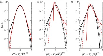
and 10. Consistent with the results in Donzis & Jagannathan (Reference Donzis and Jagannathan2013), the p.d.f. of temperature is close to Gaussian at the core and is slightly skewed towards negative fluctuations for low
 $M_{t}$
but moves to the positive side at higher
 $M_{t}$
. While
 $E_{v}^{\ast }$
is related deterministically to
 $T$
, the strongly nonlinear relation between them may give rise to very different p.d.f.s depending on the range of temperatures the flow experiences. To understand this, consider for simplicity
 $e_{v}^{\ast }$
in (1.1). Because conservation of probability implies
 $f_{T}\,\text{d}T=f_{e_{v}^{\ast }}\,\text{d}e_{v}^{\ast }$
, the p.d.f. of
 $e_{v}^{\ast }$
is given by
 $(\text{d}e_{v}^{\ast }/\text{d}T)^{-1}f_{T}(T)$
. Using again (1.1) we find
 $$\begin{eqnarray}\displaystyle f_{e_{v}^{\ast }}(e_{v}^{\ast })=\frac{4}{R}\left(\frac{T}{{\it\theta}_{v}}\right)^{2}\text{sinh}^{2}\left(\frac{1}{2}\frac{{\it\theta}_{v}}{T}\right)f_{T}\left(\frac{{\it\theta}_{v}}{\ln (1+R{\it\theta}_{v}/e_{v}^{\ast })}\right)\!, & & \displaystyle\end{eqnarray}$$
where the argument of
 $f_{T}$
is
 $T$
expressed as a function of
 $e_{v}^{\ast }$
.
For very high temperatures (low
 $K_{T}$
) at which vibrational modes are fully excited, that is,
 $e_{v}^{\ast }\approx RT$
, the derivative
 $(\text{d}e_{v}^{\ast }/\text{d}T)^{-1}$
tends to
 $1/R$
and the argument of
 $f_{T}$
in (5.1) tends to
 $e_{v}^{\ast }/R$
. This implies that
 $f_{e_{v}^{\ast }}(e_{v}^{\ast })=(1/R)f_{T}(e_{v}^{\ast }/R)$
. We thus expect small differences between
 $f_{T}$
and
 $f_{e_{v}^{\ast }}$
when variables are normalized, as they are simply related by a multiplicative constant. This is in fact observed from our DNS data not only for
 $e_{v}^{\ast }$
but also for
 $E_{v}^{\ast }$
(though slightly less so than for
 $e_{v}^{\ast }$
due to density fluctuations). This is clear from a comparison between the dashed lines (low
 $K_{T}$
case) of corresponding sets in figure 3(a,b).
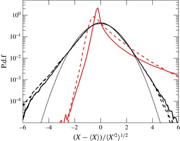
P.d.f.s of (a) temperature, (b) equilibrium vibrational energy and (c) instantaneous vibrational energy normalized by their means and standard deviations for
 $R_{{\it\lambda}}\approx 38$
. Black and red lines correspond to set 1 (SF) and set 5 (SF + EF), respectively. Line styles correspond to Gaussian (dotted),
 $K_{T}=1$
(dashed) and
 $K_{T}=10$
(solid).

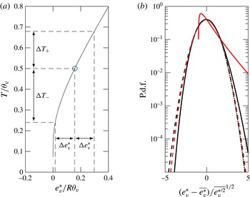
(a) Temperature as a function of equilibrium vibrational energy, i.e.
 $T/{\it\theta}_{v}=1/\log (1+R{\it\theta}_{v}/e_{v}^{\ast })$
. Similar changes in vibrational energy lead to different changes in temperature fluctuations. (b) Analytical p.d.f. of
 $e_{v}^{\ast }$
from (5.1) using the same parameters and line styles as in figure 3.

At lower temperatures (high
 $K_{T}$
), on the other hand, vibration is partially excited and
 $e_{v}^{\ast }$
is nonlinear in
 $T$
– small changes in
 $e_{v}^{\ast }$
correspond to significant changes in
 $T$
. This relation, given by (1.1), is shown in figure 4(a). Consider, as an example, a situation with
 $T/{\it\theta}_{v}=0.5$
with its corresponding value of
 $e_{v}^{\ast }$
. This condition is seen in figure 4(a) as an open circle. Now consider identical positive and negative fluctuations with magnitude
 ${\rm\Delta}e_{v}^{\ast }$
around this vibrational energy. Because of the nonlinear relation between
 $T$
and
 $e_{v}^{\ast }$
at lower temperatures, we see that a value of energy of
 $e_{v}^{\ast }(\overline{T})-{\rm\Delta}e_{v}^{\ast }$
will require stronger negative temperature fluctuations than the corresponding positive temperature fluctuation needed to observe
 $e_{v}^{\ast }(\overline{T})+{\rm\Delta}e_{v}^{\ast }$
. This effect is clear from figure 4(a), where we see
 ${\rm\Delta}T_{-}>{\rm\Delta}T_{+}$
. Furthermore, since temperature fluctuations are not far from Gaussian, the fast decay in the probability of large temperature fluctuations as
 ${\sim}\text{e}^{-T^{\prime 2}}$
suggests that even small differences between
 ${\rm\Delta}T_{-}$
and
 ${\rm\Delta}T_{+}$
(with
 ${\rm\Delta}T_{-}>{\rm\Delta}T_{+}$
) will lead to very low probabilities of strong negative vibrational energy. In other words, one would expect a strong positively skewed p.d.f. for
 $e_{v}^{\ast }$
. Note that this strong asymmetry in
 $f_{e_{v}^{\ast }}$
will be increasingly apparent for high temperature fluctuations (e.g. high
 $M_{t}$
); if temperature fluctuations are small, excursions from the mean are also small and the nonlinearities mentioned above are not seen, since locally a first-order Taylor expansion would be enough. These conclusions are indeed supported by the DNS data shown in figure 3(b). For strong temperature fluctuations (set 5 in red solid line), we observe strong non-Gaussianity and a large positive skewness. The effect is much weaker for set 1 (black solid line) which presents much smaller temperature fluctuations. Beyond predicting general trends, we further found that the analytical model (5.1) with Gaussian temperature fluctuations can indeed capture the overall behaviour of the p.d.f.s in figure 3 as seen in figure 4(b). Departures seen in the tails are associated with the slightly non-Gaussian behaviour of temperature itself for strong fluctuations (Donzis & Jagannathan Reference Donzis and Jagannathan2013).
In figure 3(c) we show
 $f_{E_{v}}$
, the p.d.f. of the instantaneous vibrational energy
 $E_{v}$
. Clearly we see the same qualitative behaviour as
 $f_{E_{v}^{\ast }}$
, though some differences are apparent. The primary reason for this is the lag between
 $E_{v}$
and
 $E_{v}^{\ast }$
noted in § 4, which precludes the former from attaining its equilibrium value. We would then expect larger differences between
 $f_{E_{v}^{\ast }}$
and
 $f_{E_{v}}$
for large
 $K_{{\it\tau}}$
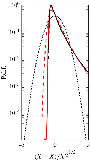
as thermal equilibrium is increasingly difficult to be attained. This is supported by figure 5, where we show the p.d.f. of
 $E_{v}$
and
 $E_{v}^{\ast }$
for different values of
 $K_{{\it\tau}}$
. As predicted, a virtual collapse between
 $f_{E_{v}^{\ast }}$
and
 $f_{E_{v}}$
is observed for small values of
 $K_{{\it\tau}}$
(black and red solid lines) since fluid elements can more quickly reach equilibrium. On the other hand, differences are clearly seen for the case with slower vibrational relaxation at
 $K_{{\it\tau}}=10$
(black and red dashed lines). The scaling of these departures with
 $K_{{\it\tau}}$
will also be analysed in more detail momentarily in spectral space.
P.d.f.s of equilibrium vibrational energy (
 $X=E_{v}^{\ast }$
) in black and instantaneous vibrational energy (
 $X=E_{v}$
) in red normalized by their mean and standard deviations for set 5 (SF + EF). Line styles correspond to Gaussian (dotted),
 $K_{{\it\tau}}=1$
(solid) and
 $K_{{\it\tau}}=10$
(dashed). The two curves for
 $E_{v}^{\ast }$
at both
 $K_{{\it\tau}}$
values overlap and are seen as one.

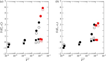
A more quantitative assessment of the scaling of these p.d.f.s can be done by investigating higher-order moments. In figure 6(a) we show the skewness factor of both
 $E_{v}^{\ast }$
and
 $e_{v}^{\ast }$
, denoted by
 $S[E_{v}^{\ast }]$
and
 $S[e_{v}^{\ast }]$
, respectively. For very small temperature fluctuations, the skewness is negative but small. This is expected since, as discussed above, small temperature fluctuations do not result in the nonlinear behaviour responsible for skewing the p.d.f. Under these conditions, then,
 $f_{e_{v}}$
is expected to exhibit similar behaviour to that of temperature fluctuations, which does present a small negative skewness (Donzis & Jagannathan Reference Donzis and Jagannathan2013). As temperature fluctuations increase, we see a different behaviour for low and high
 $K_{T}$
. Consistent with the results in figure 3, high
 $K_{T}$
leads to much stronger positive skewness. We also note that
 $S[E_{v}^{\ast }]$
is in general larger than
 $S[e_{v}^{\ast }]$
, which is again related to the general trend of thermodynamic variables, in this case density, to develop positive skewness as fluctuation levels increase (Donzis & Jagannathan Reference Donzis and Jagannathan2013). The behaviour of the skewness of the instantaneous vibrational energy (figure 6
b) is qualitatively similar, though values tend to be smaller. The reason for this behaviour is the finite-time vibrational relaxation, which prevents
 $E_{v}$
, for example, from following very strong negative or positive fluctuations in
 $E_{v}^{\ast }$
.
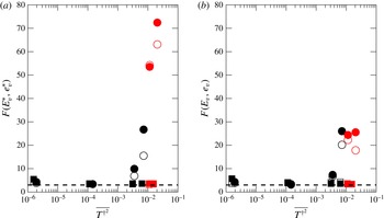
In figure 7 we show the flatness factors for the same quantities. The general trends are similar to the skewness. Flatness factors increase with
 $\overline{{T^{\dagger }}^{2}}$
as well as
 $K_{T}$
. For small temperature fluctuations, we observe flatness factors not far from the Gaussian value of 3.0, which reflect again the resemblance of vibrational energy to temperature fluctuations. We also see this behaviour for small
 $K_{T}$
when vibration is fully excited and
 $e_{v}^{\ast }$
and
 $T$
are linearly related.
Skewness of
 $E_{v}^{\ast }$
and
 $E_{v}$
(closed symbols) and of
 $e_{v}^{\ast }$
and
 $e_{v}$
(open symbols). Black and red correspond to set 1 (SF) and set 5 (SF + EF), respectively. Different symbols correspond to
 $K_{T}\sim 1$
(squares) and
 $K_{T}\sim 10$
(circles).

Flatness of
 $E_{v}$
and
 $E_{v}^{\ast }$
(closed symbols) and of
 $e_{v}$
and
 $e_{v}^{\ast }$
(open symbols). Same colours and symbols as figure 6. Horizontal dashed lines at Gaussian value of 3.0 are shown for reference.

We note that the differences in
 $E_{v}$
and
 $E_{v}^{\ast }$
will have implications in energy exchanges between translational–rotational and vibrational modes, which is represented by the last term in (4.1). In figure 8 we show the p.d.f. of this term for the same cases as in figure 3. The shape of this p.d.f. can be explained from previous results as follows. While both
 $E_{v}^{\ast }$
and
 $E_{v}$
are positively skewed, the former tends to exhibit stronger fluctuations than the latter due to the finite-time relaxation time. Therefore, we expect the difference
 $E_{v}^{\ast }-E_{v}$
to present a positive skewness for those conditions where the individual p.d.f.s are positively skewed. This is in fact what is observed in figure 8. The implication of this result is that large transfers from translational–rotational to vibrational are much more likely than the converse, especially for high
 $K_{T}$
and flows with high temperature fluctuations. As explained above, this is due to the nonlinear relation between
 $e_{v}^{\ast }$
and
 $T$
(which gives rise to asymmetric fluctuations in vibrational energy) coupled with a finite-time relaxation of vibrational non-equilibrium (which prevents
 $E_{v}$
from attaining values as high or as low as
 $E_{v}^{\ast }$
).
P.d.f. of
 $X=(E_{v}^{\ast }-E_{v})/{\it\tau}_{v}$
normalized by the mean and standard deviation for
 $R_{{\it\lambda}}\approx 38$
. Colours and line styles same as figure 3.

We finally note that, while our discussion above focused on a few selected cases in our database, we have verified that the conclusions hold equally well for all other cases in the database and are not shown for clarity. We have also found that the Reynolds number has a negligible effect on the results, at least for the conditions presented here.
5.2 Spectra
In addition to single-point statistics such as moments and p.d.f.s, DNS data can provide information about the spectral content of fluctuations in vibrational energy. This provides details about the spatial structure of the fluctuations of vibrational energy, and in particular of departures from local thermodynamic equilibrium. In § 4, we argued that, because of the finite-time relaxation of vibrational energy, temporal fluctuations in temperature will result in
 $e_{v}$
always lagging
 $e_{v}^{\ast }$
. A simple model based on a single Fourier mode in the frequency domain led to a relative departure from equilibrium given by (4.2), which shows that faster fluctuations will present greater departures from equilibrium. In order to assess the merit of such a claim with DNS data, we first note that different time scales (that is, different values of
 $1/{\it\omega}$
in the model) are associated with different length scales in a turbulent flow. Using classical phenomenology (Kolmogorov Reference Kolmogorov1941), one can estimate the velocity associated with a structure of size
 $r$
as
 $u_{r}\sim (r\langle {\it\epsilon}\rangle )^{1/3}$
. The characteristic time scale of that structure is then
 ${\it\tau}_{r}\sim r/u_{r}\sim r^{2/3}\langle {\it\epsilon}\rangle ^{-1/3}$
. Using
 $r\sim 1/k$
to relate scales in physical and wavenumber space, we can now write the ratio of time scales
 ${\it\tau}_{v}/{\it\tau}_{r}\sim {\it\tau}_{v}k^{2/3}\langle {\it\epsilon}\rangle ^{1/3}\sim K_{{\it\tau}}(k{\it\eta})^{2/3}$
. The last step was obtained using the definitions of the Kolmogorov scales and the parameter
 $K_{{\it\tau}}$
. We finally use this in (4.2) to obtain
 $$\begin{eqnarray}\displaystyle \frac{{\rm\Delta}F_{v}(k)}{F_{v}^{\ast }(k)}=\frac{c_{1}K_{{\it\tau}}^{2}(k{\it\eta})^{4/3}}{1+c_{2}K_{{\it\tau}}^{2}(k{\it\eta})^{4/3}}, & & \displaystyle\end{eqnarray}$$
where
 ${\rm\Delta}F_{v}(k)$
is the spectrum of the difference
 $E_{v}^{\ast }-E_{v}$
and
 $F_{v}^{\ast }(k)$
is the spectrum of the equilibrium vibrational energy. Equation (5.2) is the analogue of (4.2) in wavenumber space. The constants
 $c_{1}$
and
 $c_{2}$
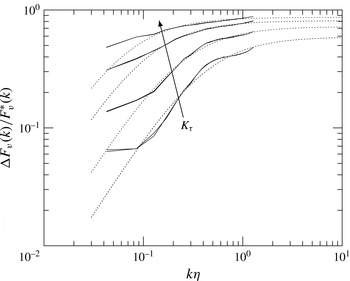
contain all order-one constants ignored in the derivation. In figure 9 we show
 ${\rm\Delta}F_{v}(k)/F_{v}^{\ast }(k)$
for different values of
 $K_{{\it\tau}}$
from our DNS database. It is clear that
 ${\rm\Delta}F_{v}(k)/F_{v}^{\ast }(k)$
increases at high wavenumbers, supporting the previous claim that there are larger departures from equilibrium at smaller (faster) scales. We can also see that (5.2) provides a good representation of the DNS data, with
 $c_{1}$
and
 $c_{2}$
being best-fit coefficients found to be of order unity for all cases. The departures observed at low wavenumbers are not unexpected since (5.2) is based on estimates valid only in the universal range, that is, for scales much smaller than integral scales. We can also see that, while for intermediate wavenumbers larger
 $K_{{\it\tau}}$
implies larger departures, at very high wavenumbers this difference shrinks. This is also consistent with the simple model in (5.2).
Relative departure from thermal equilibrium as a function of scale:
 ${\rm\Delta}F_{v}(k)/F_{v}^{\ast }(k)$
is shown for set 1 with
 $M_{t}\sim 0.1$
at
 $K_{{\it\tau}}=1$
, 2, 5 and 10.

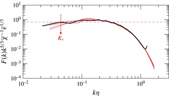
We finally note that, since (4.1) resembles the evolution equation for a passive scalar advected by the flow, one can expect well-known results for scalars such as the spectral behaviour to apply, at least in an approximate manner. Indeed, in figure 10 we show that the spectrum of
 $E_{v}$
normalized according to Obukhov–Corrsin scaling (Obukhov Reference Obukhov1949; Corrsin Reference Corrsin1951) agrees with passive scalars in incompressible flows at the same Reynolds and Prandtl numbers. We see universality at small scales as flows with different
 $K_{{\it\tau}}$
collapse into a single curve including also scalars in incompressible turbulence. In the inertial–convective range, the Obukhov–Corrsin constant
 $C_{OC}$
also compares well with values in the literature (Donzis, Sreenivasan & Yeung Reference Donzis, Sreenivasan and Yeung2010). At large scales, we see some dependence on
 ${\it\tau}_{v}$
, which is not unexpected. The Landau–Teller term acts as an effective broadband forcing for the scalar due to temperature fluctuations. As is well known, large scales are more dependent on the details of the forcing, which in our case are changed through variations in the characteristic vibrational time scale.
Red lines: the spectrum of
 $E_{v}$
,
 $F(k)$
, normalized according to Obukhov–Corrsin (
 $F(k)k^{5/3}\overline{{\it\chi}}^{-1}\overline{{\it\epsilon}}^{1/3}$
, with
 $\overline{{\it\chi}}$
and
 $\overline{{\it\epsilon}}$
being the mean dissipation rate of fluctuations in
 $E_{v}$
and kinetic energy, respectively) at
 $R_{{\it\lambda}}\approx 60$
,
 $M_{t}\approx 0.3$
and
 $K_{{\it\tau}}=0.9$
, 1.8, 4.4 and 8.8. Black line: scalar spectrum in incompressible turbulence at similar Reynolds and Prandtl numbers (Donzis et al.
Reference Donzis, Sreenivasan and Yeung2010). Horizontal dashed line:
 $C_{OK}=0.67$
for reference.

6 Summary and remarks
We presented results on general characteristics of turbulent flows when internal molecular energy modes have to be taken into account, a situation that arises in practical applications as well as in laboratory flows but that has received relatively little attention. This seems to be the first systematic study of energy distributions for these flows. We have presented theoretical arguments and direct numerical simulations to quantify the degree of the interaction and the consequences on the statistics of a canonical stationary flow, namely forced isotropic turbulence.
We have used large-scale forcing of different natures (solenoidal versus dilatational) as well as in different equations (momentum versus internal energy) to assess universality, as, in real applications, the input of energy may comprise combinations of these. We presented formulations that show robustness to different forcings, with simplifications when fluctuations of density and temperature, for example, can be related.
The strongly nonlinear nature of partially excited vibrational energy with temperature, as described by quantum mechanics, results in steady states for turbulent flows that depart from their non-fluctuating counterparts. In particular, when the mean translational temperature is the same, turbulent flows store a larger fraction of energy in vibration than flows without temperature fluctuations. This is the case in situations when there is complete thermal equilibrium as well as situations with TNE. However, the degree of departure is stronger for the latter. This phenomenon may be used, for example, to control heat transfer to surfaces in supersonic vehicles by taking advantage of the increased energy stored in vibrational, instead of translational, modes, as turbulent fluctuations increase. Quantifying the effect of turbulence on the mean vibrational energy can also be valuable in interpreting averaged experimental results of this energy mode.
To understand the nature of the fluctuations in vibrational energy, we extended our investigation to high-order moments as well as the entire probability density functions of instantaneous (
 $E_{v}$
) and equilibrium (
 $E_{v}^{\ast }$
) vibrational energy. Their p.d.f.s are found to be positively skewed and with long positive tails, an effect much more prevalent at high
 $K_{T}$
and in flows with strong temperature fluctuations. The skewness in equilibrium vibrational energy can be explained by the strongly nonlinear relation between
 $e_{v}$
and
 $T$
from quantum mechanics when vibration is partially excited. Our analytical expressions capture this effect even when temperature fluctuations are symmetric. Owing to the finite-time relaxation of vibration towards equilibrium, the p.d.f. of
 $E_{v}$
, though skewed, presents a weaker departure from symmetry. The difference between
 $E_{v}$
and
 $E_{v}^{\ast }$
has implications in energy transfers. In particular, we found that, for high
 $K_{T}$
and temperature fluctuations, strong energy transfers from translational–rotational modes to vibrational modes are much more prevalent than in the opposite direction.
Finally, we presented a simple model of the dynamics of the relaxation process which can explain a number of observations such as the persistent departures from equilibrium and the manner in which these departures manifest themselves at different scales. A main result is that departures from thermal equilibrium are stronger at smaller scales and, as expected, for relatively longer relaxation times (high
 $K_{{\it\tau}}$
). The simple model presented can indeed describe quantitatively this scale-dependent thermal non-equilibrium. We have further shown that the fluctuations of vibrational energy can be described with the classical Obukhov–Corrsin phenomenology for passive scalars for the conditions presented here. In particular, the spatial structure of fluctuations can be well described with a universal spectrum normalized according to Obukhov–Corrsin.
Some comments on the generality of the results can be made. First, we note that, while our results have been derived for isotropic turbulence, some of the conclusions apply equally to other more general flow configurations. For example, (3.6) and (3.12), which show that turbulent flows exhibit higher mean vibrational energy than laminar flows at the same mean temperature, are also valid inside a boundary layer at a fixed distance from the wall, when the average is taken in time. However, (3.8) and (3.13) rely on particular relations between temperature and density fluctuations and the turbulent Mach number, some of which were derived for isotropic flows (Donzis & Jagannathan Reference Donzis and Jagannathan2013), and may not be observed everywhere in a boundary layer, for example. Yet, though not in the details, the broad conclusion of higher mean vibrational energy in turbulent flows may still be valid in more complex situations. Clearly, further experimental or computational efforts would be needed to assess the extent of such a claim.
Second, we have utilized the widely used Landau & Teller (Reference Landau and Teller1936) model for the molecular exchange mechanism as well as the specific form suggested therein for the characteristic relaxation time. Thus one may expect conclusions to be restricted to situations where Landau–Teller is valid. However, while there are other empirical extensions for
 ${\it\tau}_{v}$
that may represent some molecular systems better (Millikan & White Reference Millikan and White1963), general results such as (4.4) are not modified. The same is true for more general extensions or modifications to the Landau–Teller model itself (e.g. Nikitin & Troe Reference Nikitin and Troe2008). Some quantitative differences may appear in, for example, (4.10) by changing the specific form of
 ${\it\tau}_{v}$
, but qualitatively the same behaviour is expected. Thus, we believe that the conclusions presented here, based on widely used models for molecular energy exchanges, are robust to refinements in the different elements of the macroscopic description of molecular exchange mechanisms. The present work could thus be seen as a base case for future research.
Acknowledgements
The authors gratefully acknowledge support from NSF (grant no. OCI-1054966) and AFOSR (grant no. FA9550-12-1-0443). We thank R. Bowersox, S. North and W. Hase for helpful discussions on the topics of this paper.