



1. Introduction
A flow in a two-dimensional square cavity driven by a moving lid is a fundamental problem in fluid mechanics. In particular, the case of a lid moving parallel to itself in the plane of the cavity is very often considered. This flow has been widely studied for various purposes, most notably investigating eddy structures and validating numerical schemes for fluid flow (see, e.g. Moffatt Reference Moffatt1964; Burggraf Reference Burggraf1966; Pan & Acrivos Reference Pan and Acrivos1967; Ghia, Ghia & Shin Reference Ghia, Ghia and Shin1982; Schumack, Schultz & Boyd Reference Schumack, Schultz and Boyd1991; Shankar Reference Shankar1993; Srinivasan Reference Srinivasan1995; Botella & Peyret Reference Botella and Peyret1998; Shankar & Deshpande Reference Shankar and Deshpande2000).
As is well known, the solution is singular at the corners due to the imposition of the no-slip boundary condition (Moffatt Reference Moffatt2009). Specifically, the flow velocity varies significantly within an arbitrarily small distance near the upper corners between the lid and side cavity walls. The limiting value of the flow velocity at the upper corners depends on the direction of approach, although it is bounded. The stress tensor and pressure diverge in approaching the upper corners inversely with the distance
 $\tilde {r}$
from them. This divergence is non-integrable, resulting in the divergence of the total forces acting on the lid and side cavity walls. The divergence of stress, pressure and total forces implies, at least locally, difficulties in describing the lid-driven cavity flow using conventional fluid mechanics.
Hereafter, we consider a monatomic gas as a fluid. The distance from the corners at which the fluid-dynamic description becomes unreliable can be estimated from the observation that the pressure deviation from a reference pressure
 $p_{\textit{ref}}$
scales as
 $\mu U/\tilde {r}$
in Taylor’s scraping flow (Taylor Reference Taylor1962; Moffatt Reference Moffatt2009), a flow relevant to the lid-driven cavity flow. Here,
 $\mu$
denotes the viscosity and
 $U$
is the lid speed. Let us use the relation between the viscosity and the mean free path
 $\ell$
of gas molecules given by kinetic theory and introduce the Mach number
 $\textit{Ma}$
in terms of
 $U$
and the sound speed at the cavity-wall temperature. Then, we recognise that the magnitude of the pressure deviation is expressed as
 $\mu U/\tilde {r} \propto \textit{Ma}p_{\textit{ref}}\ell /\tilde {r}$
. This implies that it is within a region of size comparable to the mean free path near the upper corners (
 $\tilde {r} \lesssim \ell$
) that the conventional fluid-dynamic description of the gas behaviour would break down. In general, phenomena on the mean-free-path scale are well described by kinetic theory. Thus, it may also give a more reliable description of the gas behaviour near the corners that is considered here.
There are several kinetic theory studies investigating the lid-driven flow in a rectangular cavity in the past two decades. Naris & Valougeorgis (Reference Naris and Valougeorgis2005) mainly reports on the vortex structure. In the case of John et al. (Reference John, Gu and Emerson2010, Reference John, Gu and Emerson2011) and Mohammadzadeh et al. (Reference Mohammadzadeh, Roohi, Niazmand, Stefanov and Myong2012), heat transfer is investigated and the occurrence of non-Fourier-type heat flux from low- to high-temperature regions in the rarefied regime is pointed out. Wu, Reese & Zhang (Reference Wu, Reese and Zhang2014) and Wang et al. (Reference Wang, Su, Zhu and Zhang2019) examine unsteady flow, heat transfer and damping forces induced by an oscillatory lid motion. The cavity flow is used as a benchmark problem to validate the proposed numerical methods in Frezzotti, Ghiroldi & Gibelli (Reference Frezzotti, Ghiroldi and Gibelli2011), Kloss, Shuvalov & Tcheremissine (Reference Kloss, Shuvalov and Tcheremissine2012), Guo, Xu & Wang (Reference Guo, Xu and Wang2013), Ghiroldi & Gibelli (Reference Ghiroldi and Gibelli2014), Ho et al. (Reference Ho, Li, Wu, Reese and Zhang2019) and Zhang et al. (Reference Zhang, Ma, Lou and Zhang2023). These works commonly focus on non-equilibrium effects, or non-fluid-dynamic effects, occurring in the bulk. The magnitude of these effects is characterised by the Knudsen number, the ratio of the mean free path to the cavity size.
While the characteristics of gas flows over a wide range of Knudsen numbers are analysed in the above works, investigations of the gas behaviour near the corners, or of the corner singularity, have not been reported, despite the expected advantages of kinetic theory in describing them. In this context, a cavity flow induced by a spanwise lid motion was recently investigated as a first step in Hattori (Reference Hattori2024). As indicated by the term spanwise, this work considers the lid motion in the direction perpendicular to the plane of the cavity. This setting was adopted because it is simpler than the conventional cavity flow and the corner singularity of interest arises regardless of the direction of lid motion. This simplification enabled accurate observation of the gas behaviour near the corner, and it was demonstrated that, in contrast to the conventional fluid-dynamic description, both the stress and the total forces acting on the surfaces remain finite within kinetic theory. However, in the setting, due to the spanwise lid motion, only the shear stress is non-zero among the stress components and the flow is unidirectional. Pressure variations and vortices observed in the conventional cavity flow do not manifest themselves. Thus, the flow strongly depends on the direction of lid motion. To wholly understand corner-related properties, in the present work, the analysis in the original setting is performed.
To this end, we extend the formulation and the numerical method from those in Hattori (Reference Hattori2024). In addition to examining the finiteness of the stress, pressure and total force, as well as the direction-dependent limiting values of the macroscopic quantities near the corners, corner vortices are also investigated. In conventional fluid mechanics, it is theoretically shown that they appear as an infinite series of vortices rotating in alternating directions, with decreasing size and rapidly diminishing strength, a phenomenon that has attracted attention for many years (Moffatt vortices; see, e.g. Moffatt Reference Moffatt1964; Pan & Acrivos Reference Pan and Acrivos1967; Shankar Reference Shankar1993; Biswas & Kalita Reference Biswas and Kalita2018). In the present work we examine, based on kinetic theory, effects of finite Knudsen number on this property, specifically whether corner vortices exist for a given Knudsen number, and if they do, whether their number is finite or infinite.
The paper is organised as follows. In § 2, the problem is stated and formulated as a boundary-value problem of a kinetic equation. This problem is reduced to a system of linear integral equations for macroscopic quantities, which is advantageous for accurate numerical analysis. Before proceeding to the analysis, the Stokes solution under the no-slip condition is summarised in § 3. We explicitly confirm the direction dependence of the flow velocity and the divergence of the stress and pressure at the upper corners in the Stokes solution. Section 4 presents the numerical results. As the main interest lies in the fluid-dynamic circumstances, we focus primarily on the results for small Knudsen numbers. The results imply that corner vortices arise at small Knudsen numbers and that, for a fixed Knudsen number, their number is finite. These features could not be examined in the previous work (Hattori Reference Hattori2024) due to the simplified spanwise configuration. The macroscopic quantities exhibit direction-dependent limiting values at both the upper and lower corners in the kinetic solution; their physical mechanisms and dependence on the Knudsen number are also clarified, which were beyond the scope of the previous work. The pressure, stress and, hence, the total forces acting on the lid and side walls remain finite, and the dependence of the total forces on the Knudsen number is also examined. These qualitative features are also observed in the previous work despite differences in the set of stress components considered, force directions and the presence of pressure variations, thereby indicating a certain generality of the gas behaviour near cavity corners. The paper is concluded in § 5.
2. Formulation
2.1. Problem and assumptions
Consider a gas in a cavity with a square cross-section
 $-L/2 \lt X_{1} \lt L/2$
,
 $-L/2 \lt X_{2} \lt L/2$
, where
 $X_{i}$
are the Cartesian coordinates (see figure 1). The cavity is infinitely long in the
 $X_{3}$
direction. Its upper part (
 $X_{2} = L/2$
) is closed by a planar lid moving at a constant speed
 $U_{w}$
in the
 $X_{1}$
direction. The lid and cavity walls are kept at a common uniform temperature
 $T_{0}$
. The average density of the gas over the cross-section is
 $\rho _{0}$
. No external force acts on the gas. In comparison with Hattori (Reference Hattori2024), the geometry is identical, whereas the lid motion is in a different direction. We investigate the steady behaviour of the gas under the assumptions that (i) the behaviour of the gas is described by the Bhatnagar–Gross–Krook (BGK) equation (Bhatnagar, Gross & Krook Reference Bhatnagar, Gross and Krook1954; Welander Reference Welander1954); (ii) the gas molecules are diffusely reflected on the surface of the lid and cavity walls; (iii) the lid speed
 $U_{w}$
is so small compared with the most probable speed
 $(2RT_{0})^{1/2}$
of gas molecules that the equation and boundary condition can be linearised around a uniform equilibrium state at rest with density
 $\rho _{0}$
and temperature
 $T_{0}$
, where
 $R$
denotes the specific gas constant.
Sketch of the problem.

2.2. Basic equation and boundary condition
We denote by
 $X_{i}=Lx_{i}$
(
 $i = 1, 2, 3$
) the position, by
 $(2RT_{0})^{1/2}\boldsymbol{\zeta }$
(or
 $(2RT_{0})^{1/2}\zeta _{i}$
) the molecular velocity, by
 $\rho _{0}(2RT_{0})^{-3/2}E(\zeta )[1+\phi (x_{1},x_{2},\boldsymbol{\zeta })]$
the velocity distribution function (VDF) of gas molecules and by
 $U_{w} = (2RT_{0})^{1/2}u_{w}$
the lid speed, where
 $E(\zeta ) = \pi ^{-3/2}{\rm e}^{-\zeta ^{2}}$
and
 $\zeta = |\boldsymbol{\zeta }|$
. Moreover, let us denote by
 $\rho _{0}[1+\omega (x_{1},x_{2})]$
the density of the gas, by
 $(2RT_{0})^{1/2}u_{i}(x_{1},x_{2})$
the flow velocity, by
 $T_{0}[1+\tau (x_{1},x_{2})]$
the temperature, by
 $p_{0}[1+P(x_{1},x_{2})]$
the pressure and by
 $p_{0}[\delta _{\textit{ij}}+P_{\textit{ij}}(x_{1},x_{2})]$
the stress tensor, respectively. Here,
 $p_{0} = \rho _{0}RT_{0}$
is the reference pressure and
 $\delta _{\textit{ij}}$
is the Kronecker delta.
From the assumptions (i)–(iii) in § 2.1, the behaviour of the gas is described by the boundary-value problem of the linearised BGK equation for the VDF
 $\phi (x_{1},x_{2},\boldsymbol{\zeta })$
:
 \begin{align} \zeta _{1}\frac {\partial \phi }{\partial x_{1}} + \zeta _{2}\frac {\partial \phi }{\partial x_{2}} &= \frac {1}{k}\left [\omega + 2\zeta _{j}u_{j} + \tau \left (\zeta ^{2}-\frac {3}{2}\right ) - \phi \right ] \big [(x_{1}, x_{2}) \in \varOmega ,\ \boldsymbol{\zeta } \in \mathbb{R}^{3}\big ], \\[-10pt] \nonumber \end{align}
 \begin{align} \omega &= \int \phi E \mathrm{d} \boldsymbol{\zeta }, \\[-10pt] \nonumber \end{align}
 \begin{align} u_{j} &= \int \zeta _{j}\phi E \mathrm{d} \boldsymbol{\zeta }, \\[-10pt] \nonumber\end{align}
 \begin{align} \tau &= \frac {2}{3}\int \left (\zeta ^{2}-\frac {3}{2}\right )\phi E \mathrm{d} \boldsymbol{\zeta }, \\[-10pt] \nonumber \end{align}
 \begin{align} k &= \frac {\sqrt {\pi }}{2}\textit{Kn}, \quad \textit{Kn} = \frac {\ell _{0}}{L}, \quad \ell _{0} = \frac {(8RT_{0}/\pi )^{1/2}}{A_{\textit{c}}\rho _{0}}, \\[-10pt] \nonumber \end{align}
 \begin{align} \text{b.c.} \quad \phi &= \sigma + 2\zeta _{1}u_{w}\chi _{\textit{U}} \quad [(x_{1},x_{2}) \in \partial \varOmega ,\ \zeta _{i}n_{i} \gt 0], \\[-10pt] \nonumber \end{align}
 \begin{align} \sigma &= -2\sqrt {\pi }\int _{\zeta _{j}n_{j}\lt 0} \zeta _{i}n_{i}\phi E \mathrm{d} \boldsymbol{\zeta } \quad [(x_{1},x_{2}) \in \partial \varOmega ]. \\[10pt] \nonumber \end{align}
In the above,
 $\varOmega$
and
 $\partial \varOmega$
correspond to the cross-section of the cavity and its boundary, respectively, and
 $n_{i}$
is the unit vector normal to the boundary pointed to the gas:
 \begin{align} \varOmega &= \left \{(x_{1},x_{2}) \ \left | -\frac {1}{2} \lt x_{1} \lt \frac {1}{2},\ -\frac {1}{2} \lt x_{2} \lt \frac {1}{2} \right. \right \}\!, \\[-10pt] \nonumber \end{align}
 \begin{align} \partial \varOmega &= \left \{(x_{1},x_{2}) \ \left | \left (x_{1}=\pm \frac {1}{2},\ -\frac {1}{2} \lt x_{2} \lt \frac {1}{2}\right ) \text{ or } \left (-\frac {1}{2} \lt x_{1} \lt \frac {1}{2},\ x_{2}=\pm \frac {1}{2}\right ) \right. \right \}\!, \\[-10pt] \nonumber \end{align}
 \begin{align} n_{i} &= \begin{cases} \displaystyle (\mp 1, 0, 0) & \displaystyle \quad \left (x_{1}=\pm \frac {1}{2},\ -\frac {1}{2} \lt x_{2} \lt \frac {1}{2}\right )\!, \\[9pt] \displaystyle (0, \mp 1, 0) & \displaystyle \quad \left (-\frac {1}{2} \lt x_{1} \lt \frac {1}{2},\ x_{2}=\pm \frac {1}{2}\right )\!. \end{cases} \\[10pt] \nonumber \end{align}
The quantities
 $A_{\textit{c}}\rho _{0}$
and
 $\ell _{0}$
in (2.1e
) are, respectively, the collision frequency and the mean free path of gas molecules for the BGK model in the equilibrium state at rest with density
 $\rho _{0}$
and temperature
 $T_{0}$
, where
 $A_{\textit{c}}$
is a constant. The Knudsen number is denoted by
 $\textit{Kn}$
. In the boundary condition (2.1f
),
 $\chi _{\textit{U}}$
is an indicator function defined on the boundary
 $\partial \varOmega$
, which is unity on the lid,
 $-1/2 \lt x_{1} \lt 1/2$
and
 $x_{2} = 1/2$
, and vanishes elsewhere. In (2.1b
)–(2.1d
) and (2.3) appearing soon, the integration domain is the whole space of the molecular velocity
 $\boldsymbol{\zeta }$
.
Equations (2.1b
)–(2.1d
) define the perturbations of the density, flow velocity and temperature. Similarly, the perturbations of the pressure and stress tensor are defined as the following moments of the VDF
 $\phi$
:
 \begin{align} P &= \omega + \tau = \frac {2}{3}\int \zeta ^{2}\phi E \mathrm{d} \boldsymbol{\zeta }, \end{align}
 \begin{align} P_{\textit{ij}} &= 2\int \zeta _{i}\zeta _{j}\phi E \mathrm{d} \boldsymbol{\zeta }. \end{align}
The first equality in (2.3a
) represents the linearised equation of state for an ideal gas. As evident from (2.3b
),
 $P_{\textit{ij}}$
is a symmetric tensor.
We can assume without loss of generality that the solution
 $\phi (x_{1},x_{2},\zeta _{1},\zeta _{2},\zeta _{3})$
of problem (2.1) is even in the molecular velocity component
 $\zeta _{3}$
. With this assumption, the flow velocity component
 $u_{3}$
, which appears on the right-hand side of (2.1a
), and the stress components
 $P_{13}$
and
 $P_{23}$
vanish, i.e.
 \begin{equation} u_{3}(x_{1},x_{2}) \equiv 0, \qquad P_{13}(x_{1},x_{2}) \equiv 0, \qquad P_{23}(x_{1},x_{2}) \equiv 0. \end{equation}
As expected from the geometry and direction of lid motion (see also figure 1), the solution
 $\phi$
can be considered to be symmetric with respect to
 $x_{1} = 0$
as
 \begin{equation} \phi (x_{1},x_{2},\zeta _{1},\zeta _{2},\zeta _{3}) = -\phi (-x_{1},x_{2},-\zeta _{1},\zeta _{2},\zeta _{3}). \end{equation}
Considering (2.5), it is seen that, among the macroscopic quantities, the density
 $\omega$
, flow velocity component
 $u_{2}$
, temperature
 $\tau$
, diagonal stress components
 $P_{11}$
,
 $P_{22}$
and
 $P_{33}$
and the function
 $\sigma$
in the boundary condition (2.1f
) are all odd in
 $x_{1}$
, whereas the flow velocity component
 $u_{1}$
and the shear stress component
 $P_{12}$
are even in
 $x_{1}$
:
 \begin{align} &g(x_{1},x_{2}) = -g(-x_{1},x_{2}) \quad [g = \omega , u_{2}, \tau , P_{11}, P_{22}, P_{33};\ (x_{1}, x_{2}) \in \varOmega ], \end{align}
 \begin{align} &\sigma (x_{1},x_{2}) = -\sigma (-x_{1},x_{2}) \quad [(x_{1}, x_{2}) \in \partial \varOmega ], \end{align}
 \begin{align} &g(x_{1},x_{2}) = g(-x_{1},x_{2}) \quad [g = u_{1}, P_{12};\ (x_{1}, x_{2}) \in \varOmega ]. \end{align}
Before closing this subsection, we briefly comment on the difference from the previous work (Hattori Reference Hattori2024). In that work, the spanwise flow was induced, and thus, the non-zero macroscopic quantities were limited to its speed
 $u_{3}$
and the shear stress components
 $P_{13}$
and
 $P_{23}$
, which vanish in the present problem. In contrast, in the present problem, the flow develops within the cross-section, and the in-plane velocity components
 $u_{1,2}$
, pressure
 $P$
, normal stress components
 $P_{11,22,33}$
, density
 $\omega$
and temperature
 $\tau$
become non-zero.
2.3. Integral equations
In the present problem (2.1), the boundary velocity is discontinuous at the upper corners
 $(x_{1},x_{2}) = (\pm 1/2, 1/2)$
: it is
 $(u_{w},0)$
on the lid
 $(x_{1},1/2)$
and
 $(0,0)$
on the side walls
 $(\pm 1/2,x_{2})$
. Then, the boundary condition (2.1f
) is also discontinuous, and hence, the VDF
 $\phi (x_{1},x_{2},\zeta _{1},\zeta _{2},\zeta _{3})$
is discontinuous for
 $\zeta _{1} \lessgtr 0$
,
 $\zeta _{2} \lt 0$
at the upper corners
 $(\pm 1/2, 1/2)$
. This discontinuity propagates along the characteristic lines of (2.1a
) that pass through the upper corners, which complicates the analysis. Fortunately, for the case of the linearised BGK equation with the diffuse reflection condition, which is adopted here also, this difficulty can be avoided by reducing the problem to a system of linear integral equations for macroscopic quantities (see, e.g. Hasegawa & Sone Reference Hasegawa and Sone1988; Aoki, Sone & Yano Reference Aoki, Sone and Yano1989; Sone Reference Sone2007; Taguchi & Charrier Reference Taguchi and Charrier2008). First, integrating (2.1a
) along its characteristic lines under the boundary condition (2.1f
) allows us to express
 $\phi$
in terms of the density
 $\omega$
, flow velocity components
 $u_{1}$
and
 $u_{2}$
, temperature
 $\tau$
and the function
 $\sigma$
in (2.1f
). Here, note that
 $u_{3} \equiv 0$
by (2.4). Substituting this result into (2.1b
), (2.1c
) (
 $j = 1,2$
), (2.1d
) and the definition (2.1g
) of
 $\sigma$
to eliminate the VDF
 $\phi$
, and then carrying out the integration over the molecular velocity
 $\boldsymbol{\zeta }$
, we obtain the following integral equations for the macroscopic quantities
 $\omega (\boldsymbol{x})$
,
 $u_{1}(\boldsymbol{x})$
,
 $u_{2}(\boldsymbol{x})$
,
 $\tau (\boldsymbol{x})$
and
 $\sigma (\boldsymbol{x})$
:
 \begin{align} h(\boldsymbol{x}) - A[h](\boldsymbol{x}) - A_{w}[\sigma ](\boldsymbol{x}) &= u_{w} a(\boldsymbol{x}) \quad (\boldsymbol{x} \in \varOmega ), \end{align}
 \begin{align} \sigma (\boldsymbol{x}) - B[h](\boldsymbol{x}) - B_{w}[\sigma ](\boldsymbol{x}) &= u_{w} b(\boldsymbol{x}) \quad (\boldsymbol{x} \in \partial \varOmega ). \end{align}
Here,
 $\boldsymbol{x} = (x_{1}, x_{2})$
is the position and
 $h(\boldsymbol{x}) = [\omega (\boldsymbol{x}) \ u_{1}(\boldsymbol{x}) \ u_{2}(\boldsymbol{x}) \ \tau (\boldsymbol{x})]^{\mathrm{T}}$
collectively represents the macroscopic quantities, all defined in the gas domain
 $\varOmega$
, as the column vector. The function
 $\sigma (\boldsymbol{x})$
, unlike
 $h$
, is defined only on the boundary surface
 $\partial \varOmega$
and, hence, enters the equations independently, rather than being included in
 $h$
. Below, the definitions of the linear integral operators
 $A$
,
 $A_{w}$
,
 $B$
and
 $B_{w}$
and the source terms
 $u_{w} a(\boldsymbol{x})$
and
 $u_{w} b(\boldsymbol{x})$
are given. Since this involves rather long expressions, we first explain the notation. In addition to the position
 $\boldsymbol{x} = (x_{1}, x_{2})$
, we denote by
 $\bar {\boldsymbol{x}} = (-x_{1},x_{2})$
its mirror image, by
 $\boldsymbol{x}_{*} = (x_{1*}, x_{2*})$
the integration variable and by
 $\boldsymbol{x}_{*}^{(U)} = (x_{1*}, 1/2)$
the position on the lid; they are two-dimensional vectors in the
 $x_{1}x_{2}$
plane. We denote by
 $\mathrm{d} \boldsymbol{x}_{*} = \mathrm{d} x_{1*} \mathrm{d} x_{2*}$
a surface element and by
 $\mathrm{d} l(\boldsymbol{x}_{*})$
a line element along the boundary at
 $\boldsymbol{x}_{*}$
. The right halves of the cavity cross-section
 $\varOmega$
and the cavity boundary
 $\partial \varOmega$
are denoted respectively by
 $\varOmega _{\textit{R}}$
and
 $\partial \varOmega _{\textit{R}}$
:
 $\varOmega _{\textit{R}} = \{ (x_{1},x_{2}) \ | \ (x_{1},x_{2}) \in \varOmega ,\ 0 \lt x_{1} \lt 1/2 \}$
,
 $\partial \varOmega _{\textit{R}} = \{ (x_{1},x_{2}) \ | \ (x_{1},x_{2}) \in \partial \varOmega ,\ 0 \lt x_{1} \le 1/2 \}$
. With the introduction of the column vector
 $h$
, matrix and vector notation will be used, and we also use a symbol
 $\circ$
denoting the elementwise product of two matrices (or two vectors). Now, the operators
 $A$
,
 $A_{w}$
,
 $B$
and
 $B_{w}$
and the functions
 $a(\boldsymbol{x})$
and
 $b(\boldsymbol{x})$
are given by
 \begin{align} A[h](\boldsymbol{x}) &= \frac {1}{k\pi }\int _{\varOmega } \frac {1}{|\boldsymbol{x}_{*}-\boldsymbol{x}|}K(\boldsymbol{x}_{*}-\boldsymbol{x})h(\boldsymbol{x}_{*}) \mathrm{d} \boldsymbol{x}_{*} \nonumber \\ &= \frac {1}{k\pi }\int _{\varOmega _{\textit{R}}} \bigg \{\frac {1}{|\boldsymbol{x}_{*}-\boldsymbol{x}|}K(\boldsymbol{x}_{*}-\boldsymbol{x})h(\boldsymbol{x}_{*})\nonumber \\ &\quad +\frac {1}{|\boldsymbol{x}_{*}-\bar {\boldsymbol{x}}|}\Big [S_{K} \circ K(\boldsymbol{x}_{*}-\bar {\boldsymbol{x}})\Big ]\Big [S_{h}\circ h(\boldsymbol{x}_{*})\Big ]\bigg \} \mathrm{d} \boldsymbol{x}_{*}, \end{align}
 \begin{align} \notag\\ K(\boldsymbol{z}) &= [K_{\textit{ij}}(\boldsymbol{z})] \quad (i,j = 1, 2, 3, 4), \nonumber \\ K_{11}(\boldsymbol{z}) &= J_{0}(|\boldsymbol{z}|/k), \ \ K_{12}(\boldsymbol{z}) = -2r_{1}(\boldsymbol{z})J_{1}(|\boldsymbol{z}|/k), \nonumber \\ K_{13}(\boldsymbol{z}) &= -2r_{2}(\boldsymbol{z})J_{1}(|\boldsymbol{z}|/k), \ \ K_{14}(\boldsymbol{z}) = J_{2}(|\boldsymbol{z}|/k)-J_{0}(|\boldsymbol{z}|/k), \nonumber \\ K_{21}(\boldsymbol{z}) &= -r_{1}(\boldsymbol{z})J_{1}(|\boldsymbol{z}|/k), \ \ K_{22}(\boldsymbol{z}) = 2r_{1}^{2}(\boldsymbol{z})J_{2}(|\boldsymbol{z}|/k), \nonumber \\ K_{23}(\boldsymbol{z}) &= 2r_{1}(\boldsymbol{z})r_{2}(\boldsymbol{z})J_{2}(|\boldsymbol{z}|/k), \ \ K_{24}(\boldsymbol{z}) = -r_{1}(\boldsymbol{z})[J_{3}(|\boldsymbol{z}|/k)-J_{1}(|\boldsymbol{z}|/k)], \nonumber \\ K_{31}(\boldsymbol{z}) &= -r_{2}(\boldsymbol{z})J_{1}(|\boldsymbol{z}|/k), \ \ K_{32}(\boldsymbol{z}) = 2r_{1}(\boldsymbol{z})r_{2}(\boldsymbol{z})J_{2}(|\boldsymbol{z}|/k), \nonumber \\ K_{33}(\boldsymbol{z}) &= 2r_{2}^{2}(\boldsymbol{z})J_{2}(|\boldsymbol{z}|/k), \ \ K_{34}(\boldsymbol{z}) = -r_{2}(\boldsymbol{z})[J_{3}(|\boldsymbol{z}|/k)-J_{1}(|\boldsymbol{z}|/k)], \nonumber \\ K_{41}(\boldsymbol{z}) &= (2/3)[J_{2}(|\boldsymbol{z}|/k)-\!J_{0}(|\boldsymbol{z}|/k)],\!\! \ \ K_{42}(\boldsymbol{z}) = -(4/3)r_{1}(\boldsymbol{z})[J_{3}(|\boldsymbol{z}|/k)-\!J_{1}(|\boldsymbol{z}|/k)], \nonumber \\ K_{43}(\boldsymbol{z}) &= -(4/3)r_{2}(\boldsymbol{z})[J_{3}(|\boldsymbol{z}|/k)-J_{1}(|\boldsymbol{z}|/k)], \\[-10pt] \nonumber K_{44}(\boldsymbol{z}) &= (2/3)[J_{4}(|\boldsymbol{z}|/k)-2J_{2}(|\boldsymbol{z}|/k)+(3/2)J_{0}(|\boldsymbol{z}|/k)], \\[-10pt] \nonumber \end{align}
 \begin{align} r_{i}(\boldsymbol{z}) &= \frac {z_{i}}{|\boldsymbol{z}|}, \\[-10pt] \nonumber \end{align}
 \begin{align} J_{n}(\xi ) &= \int _{0}^{\infty }t^{n}\exp \left (-t^{2}-\frac {\xi }{t}\right ) \mathrm{d} t \quad (\xi \ge 0), \\[-10pt] \nonumber \end{align}
 \begin{align} S_{K} &= \begin{bmatrix} 1 & -1 & 1 & 1 \\ -1 & 1 & -1 & -1 \\ 1 & -1 & 1 & 1 \\ 1 & -1 & 1 & 1 \end{bmatrix}, \quad S_{h} = \begin{bmatrix} -1 \\ 1 \\ -1 \\ -1 \end{bmatrix} , \\[-10pt] \nonumber \end{align}
 \begin{align} A_{w}[\sigma ](\boldsymbol{x}) &= -\frac {1}{\pi }\int _{\partial \varOmega } \frac {1}{|\boldsymbol{x}_{*}-\boldsymbol{x}|}M(\boldsymbol{x}_{*}-\boldsymbol{x})r_{i}(\boldsymbol{x}_{*}-\boldsymbol{x})n_{i}(\boldsymbol{x}_{*})\sigma (\boldsymbol{x}_{*}) \mathrm{d} l(\boldsymbol{x}_{*}) \nonumber \\ & = -\frac {1}{\pi }\int _{\partial \varOmega _{\textit{R}}}\bigg [\frac {1}{|\boldsymbol{x}_{*}-\boldsymbol{x}|}M(\boldsymbol{x}_{*}-\boldsymbol{x})r_{i}(\boldsymbol{x}_{*}-\boldsymbol{x})n_{i}(\boldsymbol{x}_{*})\sigma (\boldsymbol{x}_{*}) \nonumber \\ &\quad -\frac {1}{|\boldsymbol{x}_{*}-\bar {\boldsymbol{x}}|}[S_{M}\circ M(\boldsymbol{x}_{*}-\bar {\boldsymbol{x}})]r_{i}(\boldsymbol{x}_{*}-\bar {\boldsymbol{x}})n_{i}(\boldsymbol{x}_{*})\sigma (\boldsymbol{x}_{*})\bigg ]\mathrm{d} l(\boldsymbol{x}_{*}), \\[-10pt] \nonumber \end{align}
 \begin{align} M(\boldsymbol{z}) &= \begin{bmatrix} J_{1}(|\boldsymbol{z}|/k) \\ -r_{1}(\boldsymbol{z})J_{2}(|\boldsymbol{z}|/k) \\ -r_{2}(\boldsymbol{z})J_{2}(|\boldsymbol{z}|/k) \\ (2/3)[J_{3}(|\boldsymbol{z}|/k)-J_{1}(|\boldsymbol{z}|/k)] \end{bmatrix}, \\[-10pt] \nonumber \end{align}
 \begin{align} S_{M} &= \begin{bmatrix} 1 \\ -1 \\ 1 \\ 1 \end{bmatrix}, \\[-10pt] \nonumber \end{align}
 \begin{align} a(\boldsymbol{x}) &= \frac {1}{\pi }\int _{-1/2}^{1/2}\frac {1}{\left|\boldsymbol{x}_{*}^{(U)}-\boldsymbol{x}\right|}r_{2}\left(\boldsymbol{x}_{*}^{(U)}-\boldsymbol{x}\right) \nonumber \\ &\quad \times \begin{bmatrix} -2r_{1}\left(\boldsymbol{x}_{*}^{(U)}-\boldsymbol{x}\right)J_{2}\left(\left|\boldsymbol{x}_{*}^{(U)}-\boldsymbol{x}\right|/k\right) \\[6pt] 2r_{1}^{2}\left(\boldsymbol{x}_{*}^{(U)}-\boldsymbol{x}\right)J_{3}\left(\left|\boldsymbol{x}_{*}^{(U)}-\boldsymbol{x}\right|/k\right) \\[6pt] 2r_{1}\left(\boldsymbol{x}_{*}^{(U)}-\boldsymbol{x}\right)r_{2}\left(\boldsymbol{x}_{*}^{(U)}-\boldsymbol{x}\right)J_{3}\left(\left|\boldsymbol{x}_{*}^{(U)}-\boldsymbol{x}\right|/k\right) \\[6pt] -(4/3)r_{1}\left(\boldsymbol{x}_{*}^{(U)}-\boldsymbol{x}\right)\left[J_{4}\left(\left|\boldsymbol{x}_{*}^{(U)}-\boldsymbol{x}\right|/k\right)-J_{2}\left(\left|\boldsymbol{x}_{*}^{(U)}-\boldsymbol{x}\right|/k\right)\right] \end{bmatrix} \mathrm{d} x_{1*}, \\[-10pt] \nonumber \end{align}
 \begin{align} B[h](\boldsymbol{x}) &= \frac {2}{k\sqrt {\pi }}\int _{\varOmega } \frac {1}{|\boldsymbol{x}_{*}-\boldsymbol{x}|}r_{i}(\boldsymbol{x}_{*}-\boldsymbol{x})n_{i}(\boldsymbol{x})W(\boldsymbol{x}_{*}-\boldsymbol{x})h(\boldsymbol{x}_{*}) \mathrm{d} \boldsymbol{x}_{*} \nonumber \\ & = \frac {2}{k\sqrt {\pi }}\int _{\varOmega _{\textit{R}}}\bigg \{\frac {1}{|\boldsymbol{x}_{*}-\boldsymbol{x}|}r_{i}(\boldsymbol{x}_{*}-\boldsymbol{x})n_{i}(\boldsymbol{x})W(\boldsymbol{x}_{*}-\boldsymbol{x})h(\boldsymbol{x}_{*}) \nonumber \\ &\quad +\frac {1}{|\boldsymbol{x}_{*}-\bar {\boldsymbol{x}}|}r_{i}(\boldsymbol{x}_{*}-\bar {\boldsymbol{x}})n_{i}(\bar {\boldsymbol{x}})\big [S_{W}\circ W(\boldsymbol{x}_{*}-\bar {\boldsymbol{x}})\big ]\big [S_{h}\circ h(\boldsymbol{x}_{*})\big ]\bigg \}\mathrm{d} \boldsymbol{x}_{*}, \\[-10pt] \nonumber \end{align}
 \begin{align} W(\boldsymbol{z}) & = \begin{bmatrix} J_{1}(|\boldsymbol{z}|/k) \\ -2r_{1}(\boldsymbol{z})J_{2}(|\boldsymbol{z}|/k) \\ -2r_{2}(\boldsymbol{z})J_{2}(|\boldsymbol{z}|/k) \\ J_{3}(|\boldsymbol{z}|/k)-J_{1}(|\boldsymbol{z}|/k) \end{bmatrix}^{\mathrm{T}}, \\[-10pt] \nonumber \end{align}
 \begin{align} S_{W} &= \begin{bmatrix} 1 & -1 & 1 & 1 \end{bmatrix}, \\[-10pt] \nonumber \end{align}
 \begin{align} B_{w}[\sigma ](\boldsymbol{x}) &= -\frac {2}{\sqrt {\pi }}\int _{\partial \varOmega } \frac {1}{|\boldsymbol{x}_{*}-\boldsymbol{x}|}r_{i}(\boldsymbol{x}_{*}-\boldsymbol{x})n_{i}(\boldsymbol{x}) \nonumber \\ &\quad \times r_{j}(\boldsymbol{x}_{*}-\boldsymbol{x})n_{j}(\boldsymbol{x}_{*})J_{2}\left (\frac {|\boldsymbol{x}_{*}-\boldsymbol{x}|}{k}\right )\sigma (\boldsymbol{x}_{*}) \mathrm{d} l(\boldsymbol{x}_{*}) \nonumber \\ & = -\frac {2}{\sqrt {\pi }}\int _{\partial \varOmega _{\textit{R}}}\bigg [\frac {1}{|\boldsymbol{x}_{*}-\boldsymbol{x}|}r_{i}(\boldsymbol{x}_{*}-\boldsymbol{x})n_{i}(\boldsymbol{x}) \nonumber \\ &\quad \times r_{j}(\boldsymbol{x}_{*}-\boldsymbol{x})n_{j}(\boldsymbol{x}_{*})J_{2}\left (\frac {|\boldsymbol{x}_{*}-\boldsymbol{x}|}{k}\right )\sigma (\boldsymbol{x}_{*}) \nonumber \\ &\quad -\frac {1}{|\boldsymbol{x}_{*}-\bar {\boldsymbol{x}}|}r_{i}(\boldsymbol{x}_{*}-\bar {\boldsymbol{x}})n_{i}(\bar {\boldsymbol{x}}) r_{j}(\boldsymbol{x}_{*}-\bar {\boldsymbol{x}})n_{j}(\boldsymbol{x}_{*})J_{2}\left (\frac {|\boldsymbol{x}_{*}-\bar {\boldsymbol{x}}|}{k}\right )\sigma (\boldsymbol{x}_{*})\bigg ] \mathrm{d} l(\boldsymbol{x}_{*}), \\[-10pt] \nonumber \end{align}
 \begin{align} b(\boldsymbol{x}) &= -\frac {4}{\sqrt {\pi }}\int _{-1/2}^{1/2}\frac {1}{|\boldsymbol{x}_{*}^{(U)}-\boldsymbol{x}|}r_{i}\left(\boldsymbol{x}_{*}^{(U)}-\boldsymbol{x}\right)n_{i}(\boldsymbol{x}) \nonumber \\ &\quad \times r_{1}\left(\boldsymbol{x}_{*}^{(U)}-\boldsymbol{x}\right)r_{2}\left(\boldsymbol{x}_{*}^{(U)}-\boldsymbol{x}\right)J_{3}\Big (\frac {|\boldsymbol{x}_{*}^{(U)}-\boldsymbol{x}|}{k}\Big ) \mathrm{d} x_{1*}. \end{align}
Some additional notes regarding the above equations may be in order. The most right-hand side of (2.8a
) is obtained by splitting the integral over the cavity into its right half,
 $\varOmega _{\textit{R}}$
, and left half,
 $\varOmega _{\textit{L}} = \{ (x_{1},x_{2}) \ | \ (x_{1},x_{2}) \in \varOmega , -1/2 \lt x_{1} \lt 0 \}$
, and then rewriting the integral over the latter by changing the integration variable from
 $\boldsymbol{x}_{*} = (x_{1*}, x_{2*}) \in \varOmega _{\textit{L}}$
to
 $\bar {\boldsymbol{x}}_{*} = (-x_{1*}, x_{2*}) \in \varOmega _{\textit{R}}$
and then transcribing
 $\bar {\boldsymbol{x}}_{*}$
as
 $\boldsymbol{x}_{*}$
. In this process, we use the parity (2.6a
) and (2.6c
) for
 $h(\boldsymbol{x}_{*}) = [\omega (\boldsymbol{x}_{*}) \ u_{1}(\boldsymbol{x}_{*}) \ u_{2}(\boldsymbol{x}_{*}) \ \tau (\boldsymbol{x}_{*})]^{\mathrm{T}}$
in
 $x_{1*}$
, which implies that
 $h(\boldsymbol{x}_{*}) = S_{h} \circ h(\bar {\boldsymbol{x}}_{*})$
for
 $\boldsymbol{x}_{*} \in \varOmega _{\textit{L}}$
, as well as the corresponding property of the kernel function
 $K$
,
 $K(\boldsymbol{x}_{*}-\boldsymbol{x}) = S_{K} \circ K(\bar {\boldsymbol{x}}_{*}-\bar {\boldsymbol{x}})$
for
 $\boldsymbol{x}_{*} \in \varOmega _{\textit{L}}$
. The expressions on the most right-hand sides of (2.8f
), (2.8j
) and (2.8m
) are obtained in the same way. The functions
 $J_{n}$
, appearing in various places, are the Abramowitz functions, defined by (2.8d
). The source terms
 $u_{w} a(\boldsymbol{x})$
and
 $u_{w} b(\boldsymbol{x})$
are given as the integrals over the lid surface
 $-1/2 \lt x_{1*} \lt 1/2$
,
 $x_{2*} = 1/2$
(see (2.8i
) and (2.8n
)). Since the integration domains in
 $A$
,
 $B$
,
 $A_{w}$
and
 $B_{w}$
are restricted to the right half of the cavity,
 $\varOmega _{\textit{R}}$
and
 $\partial \varOmega _{\textit{R}}$
, the integral equations (2.7) can be solved within
 $\varOmega _{\textit{R}}$
and
 $\partial \varOmega _{\textit{R}}$
. In (2.7), the VDF and the molecular velocity
 $\boldsymbol{\zeta }$
are eliminated, so that the discontinuity of the VDF mentioned at the beginning of this subsection does not manifest itself. Hence, (2.7) is advantageous for accurate numerical analysis. In comparison with Hattori (Reference Hattori2024), where a single equation for the spanwise velocity component
 $u_{3}$
is obtained, the present formulation leads to coupled equations for
 $h(\boldsymbol{x})$
and
 $\sigma (\boldsymbol{x})$
, with additional quantities such as
 $r_{i}$
and
 $n_{i}$
defined in (2.8c
) and (2.2c
).
We remark that the functions
 $a(\boldsymbol{x})$
and
 $b(\boldsymbol{x})$
in (2.7) are direction dependent at the upper right corner
 $(x_{1},x_{2}) = (1/2, 1/2)$
. That is, the limiting values of
 $a$
and
 $b$
depend on the direction from which the corner is approached, which can be verified from their expressions. Then, as expected from the structure of (2.7), the solution
 $h(\boldsymbol{x}) = [\omega (\boldsymbol{x}) \ u_{1}(\boldsymbol{x}) \ u_{2}(\boldsymbol{x}) \ \tau (\boldsymbol{x})]^{\mathrm{T}}$
and
 $\sigma (\boldsymbol{x})$
can also exhibit direction-dependent limiting values at the corner. To address this property related to the corner appropriately, we introduce the following plane polar coordinates,
 $(r_{+},\varphi _{+})$
and
 $(r_{-},\varphi _{-})$
, centred at the corners (see figure 2):
 \begin{equation} x_{1} = \frac {1}{2} - r_{\pm }\cos \varphi _{\pm }, \quad x_{2} = \pm \frac {1}{2} \mp r_{\pm }\sin \varphi _{\pm } \quad \big(0 \le \varphi _{\pm } \le \pi /2\big). \end{equation}
Here,
 $r_{\pm }$
is the distance from the upper or lower right corner
 $(1/2,\pm 1/2) \equiv \boldsymbol{x}_{\textit{c}}^{\pm }$
to the point
 $\boldsymbol{x}$
, and
 $\varphi _{\pm }$
is the angle of the vector
 $\boldsymbol{x}-\boldsymbol{x}_{\textit{c}}^{\pm }$
measured from
 $x_{2} = \pm 1/2$
towards
 $x_{1} = 1/2$
. Using these coordinates, for example, the limiting values of
 $u_{i}(\boldsymbol{x})$
when the upper right corner is approached can be written as
 $\lim _{r_{+}\to 0}u_{i}(\boldsymbol{x}(r_{+},\varphi _{+}))$
with
 $\varphi _{+}$
being fixed. In this way, any potential direction dependence of macroscopic quantities is properly handled as their dependence on the azimuthal angle
 $\varphi _{\pm }$
.
Plane polar coordinates with its origin at a corner: (a) (
 $r_{+}$
,
 $\varphi _{+}$
), and (b) (
 $r_{-}$
,
 $\varphi _{-}$
).

By substituting the expression of the VDF
 $\phi$
in terms of the density
 $\omega$
, flow velocity components
 $u_{1}$
and
 $u_{2}$
, temperature
 $\tau$
and the function
 $\sigma$
, mentioned before (2.7), into (2.3b
), we obtain the following expression for the stress components
 $P_{11}$
,
 $P_{22}$
and
 $P_{12}$
:
 \begin{align} &P_{\textit{ij}}(\boldsymbol{x}) \nonumber \\ &= \frac {2}{k\pi }\int _{\varOmega }\frac {1}{|\boldsymbol{x}_{*}-\boldsymbol{x}|} \big \{ r_{i}(\boldsymbol{x}_{*}-\boldsymbol{x})r_{j}(\boldsymbol{x}_{*}-\boldsymbol{x})J_{2}(|\boldsymbol{x}_{*}-\boldsymbol{x}|/k)\omega (\boldsymbol{x}_{*}) \nonumber \\ &\quad -2r_{i}(\boldsymbol{x}_{*}-\boldsymbol{x})r_{j}(\boldsymbol{x}_{*}-\boldsymbol{x})r_{\ell }(\boldsymbol{x}_{*}-\boldsymbol{x})J_{3}(|\boldsymbol{x}_{*}-\boldsymbol{x}|/k)u_{\ell }(\boldsymbol{x}_{*}) \nonumber \\ &\quad + r_{i}(\boldsymbol{x}_{*}-\boldsymbol{x})r_{j}(\boldsymbol{x}_{*}-\boldsymbol{x})\big [J_{4}(|\boldsymbol{x}_{*}-\boldsymbol{x}|/k)-J_{2}(|\boldsymbol{x}_{*}-\boldsymbol{x}|/k)\big ]\tau (\boldsymbol{x}_{*}) \big \}\mathrm{d} \boldsymbol{x}_{*} \nonumber \\ &\quad -\frac {2}{\pi }\int _{\partial \varOmega } \frac {1}{|\boldsymbol{x}_{*}-\boldsymbol{x}|} r_{i}(\boldsymbol{x}_{*}-\boldsymbol{x})r_{j}(\boldsymbol{x}_{*}-\boldsymbol{x})J_{3}(|\boldsymbol{x}_{*}-\boldsymbol{x}|/k) r_{\ell }(\boldsymbol{x}_{*}-\boldsymbol{x})n_{\ell }(\boldsymbol{x}_{*})\sigma (\boldsymbol{x}_{*}) \mathrm{d} l(\boldsymbol{x}_{*}) \nonumber \\ &\quad -\frac {4u_{w}}{\pi }\int _{-1/2}^{1/2} r_{i}\left(\boldsymbol{x}_{*}^{(U)}-\boldsymbol{x}\right)r_{j}\left(\boldsymbol{x}_{*}^{(U)}-\boldsymbol{x}\right)r_{1}\left(\boldsymbol{x}_{*}^{(U)}-\boldsymbol{x}\right)r_{2}\left(\boldsymbol{x}_{*}^{(U)}-\boldsymbol{x}\right) \nonumber \\ &\quad \times J_{4}\left(\left|\boldsymbol{x}_{*}^{(U)}-\boldsymbol{x}\right|/k\right) \mathrm{d} x_{1*}. \end{align}
Here,
 $(i,j) = (1,1)$
,
 $(2,2)$
and
 $(1,2)$
. Once
 $h(\boldsymbol{x}) = [\omega (\boldsymbol{x}) \ u_{1}(\boldsymbol{x}) \ u_{2}(\boldsymbol{x}) \ \tau (\boldsymbol{x})]^{\mathrm{T}}$
and
 $\sigma (\boldsymbol{x})$
are determined by solving (2.7),
 $P_{11}$
,
 $P_{22}$
and
 $P_{12}$
follow from (2.10). Note that the present formulation also allows the stress component
 $P_{33}$
and the heat-flow vector to be obtained. However, for brevity, their expressions and results are omitted in the present paper.
The integral equations (2.7) for the macroscopic quantities
 $h(\boldsymbol{x})$
and
 $\sigma (\boldsymbol{x})$
are solved by successive approximation (Hasegawa & Sone Reference Hasegawa and Sone1988; Aoki et al. Reference Aoki, Sone and Yano1989; Sone Reference Sone2007; Taguchi & Charrier Reference Taguchi and Charrier2008). Specifically, starting from some initial guesses
 $h^{0}(\boldsymbol{x})$
and
 $\sigma ^{0}(\boldsymbol{x})$
, sequences
 $\{h^{n}\}$
and
 $\{\sigma ^{n}\}$
are constructed by the recurrence relations
 \begin{align} h^{n}(\boldsymbol{x}) &= A[h^{n-1}](\boldsymbol{x}) + A_{w}[\sigma ^{n-1}](\boldsymbol{x}) + u_{w} a(\boldsymbol{x}) \quad (\boldsymbol{x} \in \varOmega _{\textit{R}};\ n = 1, 2, \ldots ), \end{align}
 \begin{align} \sigma ^{n}(\boldsymbol{x}) &= B[h^{n-1}](\boldsymbol{x}) + B_{w}[\sigma ^{n-1}](\boldsymbol{x}) + u_{w} b(\boldsymbol{x}) \quad (\boldsymbol{x} \in \partial \varOmega _{\textit{R}};\ n = 1, 2, \ldots ), \end{align}
which correspond to (2.7). The solution
 $h(\boldsymbol{x})$
and
 $\sigma (\boldsymbol{x})$
is obtained as the limit of the sequences. In actual numerical computations based on (2.11), the integrals
 $A[h^{n-1}]$
,
 $B[h^{n-1}]$
,
 $A_{w}[\sigma ^{n-1}]$
and
 $B_{w}[\sigma ^{n-1}]$
need to be evaluated numerically using the known data
 $h^{n-1}$
and
 $\sigma ^{n-1}$
at the grid points. This is done by extending the procedure described in Hattori (Reference Hattori2024). Information on the numerical method, grid system and computational accuracy is summarised in Appendix A.1.
3. Stokes solution
Before proceeding to numerical analysis of the integral equations (2.7), we briefly present the Stokes solution under the no-slip condition. This solution has been obtained in the literature (see, e.g. Burggraf Reference Burggraf1966; Pan & Acrivos Reference Pan and Acrivos1967; Shankar Reference Shankar1993; Srinivasan Reference Srinivasan1995). Thus, it is not new in itself. However, since we extensively use it in § 4 to discuss the gas behaviour near the corner, accurate and quantitative information is required. For completeness, we outline its construction here. It is effective to extract the singular part of the solution near the upper corner and obtain the remainder numerically. After explaining this procedure, we also explicitly confirm the direction dependence of the flow velocity and the divergence of the stress and pressure at the corner in the Stokes solution, mentioned in the second paragraph of § 1.
First, in the present problem, the continuity equation, the Stokes equation and the no-slip condition are given for the flow velocity components
 $u_{1}$
and
 $u_{2}$
and the pressure
 $P$
as
 \begin{align} \partial _{x_{1}}u_{1} + \partial _{x_{2}}u_{2} &= 0 \quad [(x_{1}, x_{2}) \in \varOmega ], \end{align}
 \begin{align} \partial _{x_{i}}P &= k\Delta u_{i} \quad [i = 1, 2;\ (x_{1}, x_{2}) \in \varOmega ], \end{align}
 \begin{align} \text{b.c.} \quad u_{i} &= u_{w}\delta _{i1}\chi _{\textit{U}} \quad [i = 1, 2;\ (x_{1}, x_{2}) \in \partial \varOmega ]. \end{align}
Here, the shorthand notation
 $\partial /\partial x_{i} = \partial _{x_{i}}$
is used in this section to save space; the parameter
 $k$
is defined in (2.1e
);
 $\chi _{\textit{U}}$
denotes the indicator function (see also the sentences after (2.2c
)); and
 $\varDelta = \partial _{x_{1}}^{2}+\partial _{x_{2}}^{2}$
is the Laplacian. The stress components
 $P_{\textit{ij}}$
are given in terms of
 $P$
and
 $u_{1,2}$
based on Newton’s law and the expression of the viscosity for the BGK model:
 \begin{equation} P_{\textit{ij}} = P\delta _{\textit{ij}} - k (\partial _{x_{j}}u_{i} + \partial _{x_{i}}u_{j}) \quad [(i,j) = (1,1), (2,2), (1,2)]. \end{equation}
Since the present problem is spatially two dimensional, here we introduce the streamfunction
 $\psi (x_{1},x_{2})$
and the vorticity
 $\omega (x_{1},x_{2})$
as
 \begin{equation} u_{1} = \partial _{x_{2}}\psi , \quad u_{2} = -\partial _{x_{1}}\psi , \quad \omega = \partial _{x_{1}}u_{2} - \partial _{x_{2}}u_{1}. \end{equation}
Then, the Stokes flow problem (3.1) reduces to the following problem for
 $\psi$
and
 $\omega$
:
 \begin{align} \Delta \omega &= 0, \quad \Delta \psi = - \omega \quad [(x_{1}, x_{2}) \in \varOmega ], \end{align}
 \begin{align} \text{b.c.} \quad \psi &= 0, \quad -n_{i}\partial _{x_{i}}\psi = u_{w}\chi _{\textit{U}} \quad [(x_{1}, x_{2}) \in \partial \varOmega ]. \end{align}
Below, we also use the polar coordinates centred at the upper right corner (see figure 2
a). Let us introduce the following functions of radius
 $r_{+}$
and azimuthal angle
 $\varphi _{+}$
, which correspond to the solution of Taylor’s scraping flow (Taylor Reference Taylor1962; Moffatt Reference Moffatt2009):
 \begin{align} \tilde {\psi }(r_{+}(\boldsymbol{x}), \varphi _{+}(\boldsymbol{x})) &= u_{w}r_{+}(\boldsymbol{x})f(\varphi _{+}(\boldsymbol{x})), \end{align}
 \begin{align} \tilde {\omega }(r_{+}(\boldsymbol{x}), \varphi _{+}(\boldsymbol{x})) &= -\frac {u_{w}}{r_{+}(\boldsymbol{x})}\big[f(\varphi _{+}(\boldsymbol{x})) + f^{\prime \prime }(\varphi _{+}(\boldsymbol{x}))\big], \end{align}
 \begin{align} \tilde {P}(r_{+}(\boldsymbol{x}), \varphi _{+}(\boldsymbol{x})) &= -\frac {u_{w} k}{r_{+}(\boldsymbol{x})}\big[f^{\prime \prime \prime }(\varphi _{+}(\boldsymbol{x})) + f^{\prime }(\varphi _{+}(\boldsymbol{x}))\big], \end{align}
 \begin{align} \text{with} \quad f(\varphi ) &= \frac {\varphi \cos \varphi -(\pi /2)[(\pi /2)-\varphi ]\sin \varphi }{(\pi ^{2}/4)-1}. \end{align}
Then, the streamfunction
 $\tilde {\psi }$
and the vorticity
 $\tilde {\omega }$
satisfy (3.4a
) and boundary conditions (3.4b
) on the lid and right wall within the domain
 $\varOmega _{\textit{R}}$
. The condition (3.4b
) on the bottom wall is not satisfied. The pressure
 $\tilde {P}$
corresponds to the pressure determined from the Stokes equation for the flow velocity field
 $(\partial _{x_{2}}\tilde {\psi }, -\partial _{x_{1}}\tilde {\psi })$
given by
 $\tilde {\psi }$
. Taking these into account, we expect that the functions
 $\tilde {\psi }$
and
 $\tilde {\omega }$
well represent the gas behaviour near the upper right corner, and we therefore decompose the streamfunction
 $\psi$
and the vorticity
 $\omega$
in problem (3.4) into the following known and unknown parts:
 \begin{equation} \psi (\boldsymbol{x}) = \psi ^{\dagger }(\boldsymbol{x}) + \psi ^{\#}(\boldsymbol{x}), \quad \omega (\boldsymbol{x}) = \omega ^{\dagger }(\boldsymbol{x}) + \omega ^{\#}(\boldsymbol{x}). \end{equation}
Here, the known parts of the streamfunction
 $\psi ^{\dagger }$
and the vorticity
 $\omega ^{\dagger }$
are given in terms of
 $\tilde {\psi }$
and
 $\tilde {\omega }$
in (3.5a
) and (3.5b
) as
 \begin{align} \psi ^{\dagger }(\boldsymbol{x}) &= \tilde {\psi }(r_{+}(\boldsymbol{x}), \varphi _{+}(\boldsymbol{x})) S(r_{+}(\boldsymbol{x})), \nonumber\\ \omega ^{\dagger }(\boldsymbol{x}) &= \tilde {\omega }(r_{+}(\boldsymbol{x}), \varphi _{+}(\boldsymbol{x})) S(r_{+}(\boldsymbol{x})) \quad (x_{1} \ge 0), \end{align}
 \begin{align} S(z) &= \begin{cases} \displaystyle \frac {e^{-1/(1-2z)}}{e^{-(1/2z)}+e^{-1/(1-2z)}} & \displaystyle \quad \left(z \lt \frac {1}{2}\right)\!, \\[9pt] 0 & \displaystyle \quad \left(z \ge \frac {1}{2}\right)\!, \end{cases} \end{align}
 \begin{align} \psi ^{\dagger }(x_{1},x_{2}) &= \psi ^{\dagger }(-x_{1},x_{2}), \quad \omega ^{\dagger }(x_{1},x_{2}) = \omega ^{\dagger }(-x_{1},x_{2}) \quad (x_{1} \lt 0). \end{align}
The function
 $S(r_{+})$
is a smooth function decreasing from unity to zero on
 $0 \le r_{+} \le 1/2$
. Note that this construction of known parts using
 $S$
is adopted in Hattori (Reference Hattori2024) for a cavity flow driven by a spanwise lid motion; a plot of
 $S$
is shown in figure 3 of the reference.
The remainder parts of the streamfunction and vorticity,
 $\psi ^{\#}$
and
 $\omega ^{\#}$
, are determined by the system obtained by substituting the decomposition (3.6) into the original system (3.4), namely the equations
 $\Delta \omega ^{\#} = -\Delta \omega ^{\dagger }$
and
 $\Delta \psi ^{\#} = -\omega ^{\#} - (\omega ^{\dagger } + \Delta \psi ^{\dagger })$
with the boundary conditions
 $\psi ^{\#} = -\psi ^{\dagger }$
and
 $-n_{i}\partial _{x_{i}}\psi ^{\#} = u_{w}\chi _{\textit{U}} + n_{i}\partial _{x_{i}}\psi ^{\dagger }$
. The source terms in this system behave nicely near the corner because the known parts,
 $\psi ^{\dagger }$
and
 $\omega ^{\dagger }$
given by (3.7) and (3.5), satisfy (3.4a
) and boundary conditions (3.4b
) well there. Hence, this system can be treated safely without any singular factors. Indeed, using a standard second-order central finite-difference scheme with a grid consisting of
 $1601 \times 1601$
points,
 $\psi ^{\#}$
and
 $\omega ^{\#}$
are obtained straightforwardly; see also Appendix A.2 for information on the computation.
As described above, the streamfunction
 $\psi = \psi ^{\dagger } + \psi ^{\#}$
and the vorticity
 $\omega = \omega ^{\dagger } + \omega ^{\#}$
representing the Stokes solution are obtained. The corresponding flow velocity
 $u_{i} = u_{i}^{\dagger } + u_{i}^{\#}$
, pressure
 $P = P_{}^{\dagger } + P_{}^{\#}$
and stress
 $P_{\textit{ij}} = P_{\textit{ij}}^{\dagger } + P_{\textit{ij}}^{\#}$
can then be obtained from the streamfunction. Here,
 $h^{\dagger }$
and
 $h^{\#}$
(
 $h = u_{i}, P, P_{\textit{ij}}$
) denote the known part associated with
 $\psi ^{\dagger }$
and the remainder part associated with
 $\psi ^{\#}$
, respectively. For completeness, their explicit expressions are given in Appendix B.
From the numerical results, it can be confirmed that the remainder part of the flow velocity
 $u_{i}^{\#}$
approaches zero as the upper right corner is approached (
 $r_{+} \to 0$
). On the other hand, its known part,
 $u_{i}^{\dagger }|_{r_{+}\to 0} = f^{\prime }(\varphi _{+})e_{i}^{(r_{+})}-f(\varphi _{+})e_{i}^{(\varphi _{+})}$
, depends on the azimuthal angle
 $\varphi _{+}$
. Here,
 $(e_{1}^{(r_{+})},e_{2}^{(r_{+})}) = (-\cos \varphi _{+},-\sin \varphi _{+})$
and
 $(e_{1}^{(\varphi _{+})},e_{2}^{(\varphi _{+})}) = (\sin \varphi _{+},-\cos \varphi _{+})$
are the unit vectors in the
 $r_{+}$
and
 $\varphi _{+}$
directions, respectively. Hence, the flow velocity
 $u_{i}(= u_{i}^{\dagger } + u_{i}^{\#})$
exhibits direction-dependent limiting values at the corner. Similarly, the divergence of the stress when the corner is approached can be explicitly confirmed from the expressions of the known part
 $P_{\textit{ij}}^{\dagger }$
. For brevity, here let us fix the approach direction and consider the shear stress
 $P_{12}^{\dagger }|_{\varphi _{+} = 0}$
along the lid and the stress components
 $P_{11}^{\dagger }|_{\varphi _{+} = \pi /2}$
and
 $P_{12}^{\dagger }|_{\varphi _{+} = \pi /2}$
along the right wall. These are given by
 $P_{12}^{\dagger }|_{\varphi _{+} = 0} = -ku_{w} f^{\prime \prime }(0)r_{+}^{-1}S(r_{+})$
,
 $P_{11}^{\dagger }|_{\varphi _{+} = \pi /2} = -ku_{w} [f^{\prime \prime \prime }(\pi /2)+f^{\prime }(\pi /2)]r_{+}^{-1}S(r_{+})$
and
 $P_{12}^{\dagger }|_{\varphi _{+} = \pi /2} = ku_{w} f^{\prime \prime }(\pi /2)r_{+}^{-1}S(r_{+})$
(see also (B1) and (B2b
)). Considering
 $S(0) = 1$
, all of these diverge inversely with the distance
 $r_{+}$
as
 $r_{+} \to 0$
. The total forces obtained by integrating these stresses along the surfaces also diverge. As for the stress
 $P_{22}^{\dagger }|_{\varphi _{+} = 0}$
along the lid, it also diverges as
 $r_{+} \to 0$
, but note that the corresponding total force in the
 $x_{2}$
direction remains finite because
 $P_{22}$
is odd in
 $x_{1}$
and the contributions cancel out upon integration; see (2.6a
) and (4.1b
) appearing later. From (3.5c
) and
 $P_{}^{\dagger } = \tilde {P}S$
, the pressure also diverges at the same rate
 $r_{+}^{-1}$
.
4. Numerical results and discussion
First, to grasp the overall behaviour of the gas, the flow velocity, stress and pressure fields for representative Knudsen numbers are examined in § 4.1. Then, in § 4.2 we examine the corner vortices near the lower corner, focusing on whether corner vortices exist for a given Knudsen number, and if they do, whether their number is finite or infinite. These issues could not be addressed in the previous work with a spanwise configuration (Hattori Reference Hattori2024). The direction dependence of macroscopic quantities at both the upper and lower corners is investigated in § 4.3. In the present work, the physical mechanisms underlying the differing direction-dependent behaviour of the macroscopic quantities at the upper and lower corners are also clarified, with a detailed explanation provided in Appendix C. The behaviour of macroscopic quantities near the upper corner for small Knudsen numbers and the forces acting on the lid and cavity walls are analysed in §§ 4.4 and 4.5, respectively. Compared with the previous work, different sets of macroscopic quantities are examined in the present configuration. Nevertheless, the results reveal a series of qualitative features that are consistent with those observed previously: the formation of a near-corner region in which the macroscopic quantities vary on the scale of the mean free path; the fluid-dynamic increase of stress and pressure up to distances of a few tens of mean free paths from the corner followed by a transition to a bounded profile closer to the corner; and the resulting finiteness and
 $k\ln k$
-type scaling of the total forces. These features indicate a certain generality of the gas behaviour near cavity corners. Finally, in § 4.6 we briefly discuss the implications of the present results for the validity of macroscopic fluid-dynamic descriptions.
4.1. Flow velocity, stress and pressure fields over whole cavity
Plots of the flow velocity fields and the streamlines in the cavity: (a)
 $k = 0.01$
, (b)
 $k = 1$
and (c)
 $k = 10$
. The arrows indicate the flow velocity components
 $(u_{1}/u_{w},u_{2}/u_{w})$
at their starting points with their scale being shown on the left shoulder of each panel. At the four corners
 $(\pm 1/2, \pm 1/2)$
, two values, that approached from the upper or lower boundary and that approached from the side walls are shown although they are not visible for the lower corners. Its close-up around the upper right corner is shown on the top of each panel, where the two values are indicated by arrows with filled and hollow arrowheads, respectively, the corner by a bullet, and the lid and right wall by solid lines. The solid lines represent the streamlines originating from the points
 $(0,0.15)$
,
 $(0,0)$
,
 $(0.1,-0.1)$
,
 $(0.2,-0.2)$
,
 $(0.3,-0.3)$
,
 $(0.4,-0.4)$
,
 $(0.45,-0.45)$
,
 $(0.49,-0.49)$
and
 $(-0.49,-0.49)$
.

Figure 3 shows the vector fields of the flow velocity
 $(u_{1}/u_{w},u_{2}/u_{w})$
and the streamlines for
 $k=0.01$
,
 $1$
and
 $10$
over the whole cavity cross-section. The quantities in the left half of the cavity are recovered from the numerical results in the right half by using the parity relations (2.6a
) and (2.6c
). As defined in (2.1e
),
 $k = (\sqrt {\pi }/2)\textit{Kn}$
, and hereafter the parameter
 $k$
is used instead of the Knudsen number
 $\textit{Kn}$
. As the figure indicates, a flow is induced by the lid motion and a clockwise vortex appears. For smaller
 $k$
(figure 3
a), the flow speed is faster. As
 $k$
increases, the velocity slip on the lid (
 $x_{2} = 1/2$
), i.e. the difference between the lid speed and the gas flow velocity, becomes larger, and the overall flow speed decreases. The position of the vortex centre shifts slightly downward with increasing
 $k$
. For
 $k=1$
and
 $10$
, judging from the drawn streamlines, only a single vortex is present in the cavity (figures 3
b and 3
c). On the other hand, for
 $k = 0.01$
, in addition to the primary vortex, a second small counter-rotating vortex is observed near the lower corners
 $(\pm 1/2, -1/2)$
(figure 3
a). This vortex corresponds to the Moffatt’s corner vortex in fluid mechanics. Considering the possible direction-dependent limiting values, at each corner, two representative flow velocity vectors are shown in figure 3: one with the corner being approached along the upper or lower boundary and one with the corner being approached along the side walls. At the lower corners the arrows are not visible. At the upper right corner, as shown in the close-ups, the vector points to the right along the lid when approached from the lid side, whereas it points downward along the right wall when approached from the right wall. This indicates that the flow velocity at the upper corners is actually direction dependent for various Knudsen numbers. The corner vortices near the lower corners and the direction dependence of the macroscopic quantities are further examined later in §§ 4.2 and 4.3.
Contour plots of the stress components
 $P_{12}/u_{w}$
,
 $P_{11}/u_{w}$
and
 $P_{22}/u_{w}$
and the pressure
 $P/u_{w}$
on the
 $x_{1}x_{2}$
plane for (a–d)
 $k = 0.01$
, (e–h)
 $k = 1$
, and (i–l)
 $k = 10$
. The isolines are drawn with intervals of
 $0.15$
in (b), (f) and (j), while they are drawn with intervals of
 $0.1$
in the other panels.

Figure 4 shows contour plots of the stress components
 $P_{12}/u_{w}$
,
 $P_{11}/u_{w}$
and
 $P_{22}/u_{w}$
and the pressure
 $P/u_{w}$
for
 $k=0.01$
,
 $1$
and
 $10$
. In all cases, their magnitudes are particularly large on the lid and side walls. For non-small Knudsen numbers (
 $k=1$
and
 $10$
), the variations of the macroscopic quantities are relatively mild and are observed over the whole cavity (figure 4
e–l). In contrast, when the Knudsen number is small (
 $k=0.01$
), they vary steeply near the upper corners (figure 4
a–d). The behaviour of the stress, pressure and flow velocity near the corners for small Knudsen numbers is further examined later in § 4.4. For
 $k=0.01$
, the magnitudes of the stress and pressure in the bulk away from the boundaries are smaller than those for
 $k=1$
and
 $10$
. This is consistent with the fact that their magnitudes, determined from the Stokes equation (3.1b
), Newton’s law (3.2) and a smooth
 $O(1)$
velocity distribution
 $u_{i}/u_{w}$
in the bulk, are
 $O(k)$
and are thus small.
Before closing this subsection, let us mention thermal characteristics of the gas briefly. In transition and highly rarefied regimes, the temperature
 $\tau /u_{w}$
is higher near the upper right corner and lower near the upper left corner. The heat flows from the low-temperature region to the high-temperature one, which is the so-called anti-Fourier heat transfer (see, e.g. John et al. Reference John, Gu and Emerson2010, Reference John, Gu and Emerson2011; Mohammadzadeh et al. Reference Mohammadzadeh, Roohi, Niazmand, Stefanov and Myong2012), and the present results confirm its existence even within the linearised regime. As the Knudsen number decreases, the temperature variations become increasingly confined near the upper corners. The heat-flow streamlines exhibit a more complex pattern, including the formation of a small vortex near the bottom wall. The behaviour of heat flow near the boundary is consistent with a shear-induced heat flow within the Knudsen layer. For details, including the visualised fields, the reader is referred to supplementary material S1 available at https://doi.org/10.1017/jfm.2026.11787.
4.2. Corner vortices
In conventional fluid mechanics, it is theoretically shown that corner vortices appear as an infinite series of vortices that rotate in alternating directions, with their size decreasing and their strength decaying rapidly (Moffatt vortices; see Moffatt Reference Moffatt1964). For the Stokes flow in a square cavity corresponding to the present setting, within the achievable computational accuracy, multiple corner vortices near the lower corners are actually confirmed numerically (see, e.g. Pan & Acrivos Reference Pan and Acrivos1967; Shankar Reference Shankar1993; Biswas & Kalita Reference Biswas and Kalita2018), which supports the theoretical statement. Here, we examine the effect of a finite Knudsen number on this property, specifically whether corner vortices exist for a given Knudsen number and, if they do, whether their number is finite or infinite. If figure 3 is interpreted naively, one would conclude that a single corner vortex exists for
 $k = 0.01$
, whereas no corner vortices are present for
 $k = 1$
and
 $10$
. However, since this argument may depend on the scale of the figure and the choice of the starting points of streamlines, we take an alternative viewpoint below.
Sketch of streamlines near the lower right corner
 $(1/2, -1/2)$
with the presence of a single corner vortex being assumed. The points A, B, C and D chosen in the figure are specified by the same azimuthal angle
 $\varphi _{-}$
and by their respective distances
 $r_{-}$
from the corner (see also figure 2
b). The azimuthal velocity component
 $u_{\varphi _{-}}$
will be negative at points A and B in the primary vortex and at point C on the cavity-centre side of the corner vortex, while it will be positive at point D closer to the corner.

Figure 5 is a schematic illustration of streamlines near the lower right corner
 $(1/2, -1/2)$
under an assumption that a single corner vortex is present. As indicated in the figure, if there exist vortices rotating in the opposite direction, the sign of the azimuthal velocity component
 $u_{\varphi _{-}}$
is expected to reverse, near the corner-facing side of the vortex closer to the corner, e.g. at point D in the figure, relative to its sign at other locations. Here,
 $u_{\varphi _{-}} = u_{i}e_{i}^{(\varphi _{-})}$
with
 $(e_{1}^{(\varphi _{-})},e_{2}^{(\varphi _{-})}) = (\sin \varphi _{-},\cos \varphi _{-})$
being the unit vector in the
 $\varphi _{-}$
direction.
Profiles of the azimuthal velocity component near the lower right corner
 $(1/2, -1/2)$
for
 $\varphi _{-} = \pi /4$
. The quantity
 $u_{\varphi _{-}}/u_{w}$
is plotted as a function of the distance
 $r_{-}$
from the lower right corner. Panels (a–d) show the profiles in intervals
 $0 \lt r_{-} \le 0.25$
,
 $0 \lt r_{-} \le 0.08$
,
 $0 \lt r_{-} \le 0.004$
and
 $0 \lt r_{-} \le 0.004$
, respectively. Results for different sets of
 $k$
are shown in each panel. Note that the vertical scale differs from panel to panel.

With this in mind, figure 6 shows plots of
 $u_{\varphi _{-}}$
for various
 $k$
as a function of the distance
 $r_{-}$
, with the azimuthal angle being fixed at
 $\varphi _{-} = \pi /4$
. First, for
 $k = 10$
and
 $1$
,
 $u_{\varphi _{-}}$
is clearly negative for all
 $r_{-}$
, including the corner
 $r_{-}\to 0$
(figure 6
a). This implies that, under the present setting of a square cavity closed by a moving lid, corner vortices are not observed in highly rarefied to intermediate regimes, in contrast to the fluid-dynamic regime. The feature, however, depends on geometry and setting; indeed, corner vortices in highly rarefied and free-molecular regimes are reported for gas flows in an open triangular cavity (Ben-Adva & Manela Reference Ben-Adva and Manela2026) and over a backward-facing step (Manela & Gibelli Reference Manela and Gibelli2020).
On the scale of figure 6(a), for
 $k \le 0.1$
,
 $u_{\varphi _{-}}$
approaches zero as
 $r_{-}$
decreases. Thus, we show a close-up in figure 6(b). While
 $u_{\varphi _{-}}$
remains negative over the entire range for
 $k = 0.1$
and
 $0.03$
, for
 $k = 0.02$
, there exists an interval over which
 $u_{\varphi _{-}}$
is positive. This implies, as depicted in figure 5, the emergence of a corner vortex at this Knudsen number. As
 $k$
decreases further, the profiles approach the Stokes solution. Finally, figures 6(c) and 6(d) show further close-ups. Figure 6(c) indicates that, for
 $k$
smaller than
 $k = 0.02$
and
 $0.015$
, corresponding to the transitional stage of corner-vortex growth,
 $u_{\varphi _{-}}$
at each position
 $r_{-}$
decreases monotonically as
 $k$
decreases. For
 $k = 0.003$
and
 $0.002$
,
 $u_{\varphi _{-}}$
is still positive over the entire plotted range
 $0 \lt r_{-} \le 0.004$
(figure 6
d). On the other hand, for
 $k \le 0.0015$
, there appears an interval of
 $r_{-}$
over which
 $u_{\varphi _{-}}$
becomes negative again. This implies the emergence of a second corner vortex at these Knudsen numbers.
Streamlines near the lower right corner
 $(1/2, -1/2)$
for various
 $k$
. Panels (a–d) and panels (i–l) show the region
 $0.4 \le x_{1} \le 0.5$
and
 $-0.5 \le x_{2} \le -0.4$
, while panels (e–h) and panels (m–p) provide close-ups of the region
 $0.494 \le x_{1} \le 0.5$
and
 $-0.5 \le x_{2} \le -0.494$
. The values of
 $k$
are
 $0.03$
in (a,e),
 $0.02$
in (b,f),
 $0.01$
in (c,g),
 $0.002$
in (d,h),
 $0.0015$
in (i,m),
 $0.001$
in (j,n),
 $0.0006$
in (k,o) and
 $0.0003$
in (l,p). Panels (a–d) and panels (i–l) show streamlines originating from ten points
 $(m,-m)$
, where
 $m = 0.42$
,
 $0.4325$
,
 $0.445$
,
 $0.448$
,
 $0.468$
,
 $0.475$
,
 $0.485$
,
 $0.495$
,
 $0.4975$
and
 $0.4977$
. Panels (e–h) and panels (m–p) show streamlines originating from seven points
 $(m,-m)$
, where
 $m = 0.495$
,
 $0.4957$
,
 $0.4964$
,
 $0.4972$
,
 $0.4986$
,
 $0.4994$
and
 $0.4999$
.

The behaviour of the azimuthal velocity
 $u_{\varphi _{-}}$
as a function of the distance
 $r_{-}$
from the lower right corner has been examined in figure 6. We now show in figure 7 the streamlines near the corner for various small values of
 $k$
. As seen below, the observed features are consistent with those inferred from figure 6. For
 $k = 0.03$
, the streamlines are not closed within the displayed region, and no corner vortex is observed (figures 7
a and 7
e). On the other hand, for
 $k = 0.02$
, a first corner vortex is observed, as shown in figure 7(b). Figures 7(b) and 7(f) indicate that another small vortex can also be seen very close to the corner. However, this is regarded as a remnant of the primary clockwise vortex, which originally occupied the entire region, during the growth process of the first corner vortex, rather than as a fully developed second corner vortex. For
 $k = 0.01$
and
 $0.002$
, the first corner vortex further develops and increases in size (figures 7
c and 7
d); in the latter case, it reaches approximately the same size as that for smaller
 $k$
(compare figure 7
d with figure 7
i–l). In these cases, no second corner vortex is observed. For
 $k = 0.0015$
, a structure corresponding to a second corner vortex is just beginning to emerge (figure 7
m). For
 $k = 0.001$
,
 $0.0006$
and
 $0.0003$
, a second corner vortex is clearly observed and grows in size (figure 7
n–p).
Before closing this subsection, we summarise the results. To examine the presence and structure of corner vortices, we have focused on the distribution of the azimuthal velocity (figure 6) and the streamlines (figure 7). Figure 6(a–d) indicates that, for each fixed Knudsen number, the azimuthal flow velocity component retains a constant sign over a certain range close to the corner and does not exhibit sign changes with respect to the distance
 $r_{-}$
. Thus, unless one considers the limit
 $k \to 0$
, the number of corner vortices is finite within kinetic theory. This is in contrast to the Stokes solution, for which their number is theoretically known to be infinite. According to figures 6 and 7, zero, one or two corner vortices are observed over the range of Knudsen numbers examined (
 $k \ge 0.0003$
). The presence or absence of each corner vortex at a given Knudsen number can be understood in terms of the size relationship between the mean free path and the size of each corner vortex. When the former is not small compared with the latter, rarefaction effects, such as velocity slip, allow the gas to flow tangentially along the walls, and the flow tends not to separate from the walls, suppressing the formation of corner vortices. On the other hand, when the mean free path is sufficiently small compared with the corner-vortex size, such rarefaction effects are suppressed at that scale, and the corner vortex, which is a fluid-dynamic behaviour associated with viscosity, no-slip on the walls and the geometry with a sharp corner, can develop. Our numerical results support this interpretation. Actually, no corner vortices are observed for large Knudsen numbers down to
 $k = 0.03$
. For
 $k \le 0.02$
, a first corner vortex, which is of the size slightly less than
 $0.1$
(see, e.g. figure 7
l), appears. Moreover, for
 $k \le 0.001$
, a second corner vortex, which is of the size slightly less than
 $0.006$
(see, e.g. figure 7
p), is clearly observed. Note that, when the azimuthal angle is chosen as
 $\varphi _{-} = \pi /8$
and
 $3\pi /8$
, the same properties observed for
 $\varphi _{-} = \pi /4$
in figure 6(a–d) can be confirmed. Note that, unlike the other figures, figures 6(d) and 7(l–p) contain numerical errors associated with the scale of the plots, as they focus on quantities of extremely small magnitude and streamlines corresponding to very small velocities near the corner. To allow readers to assess the magnitude of these errors, corresponding figures obtained using a coarser grid are provided in supplementary material S2; compare figures 6 and 7 and figures S.3 and S.4 in the supplementary material. Although differences are visible, they are of a magnitude that does not affect the statements made in this subsection.
4.3. Direction dependence of limiting values of macroscopic quantities at the corners
Profiles of flow velocity components and shear stress for the BGK and Stokes solutions with
 $k = 0.01$
: (a)
 $u_{1}/u_{w}$
, (b)
 $u_{2}/u_{w}$
, and (c)
 $P_{12}/u_{w}$
. The quantities are plotted as functions of the azimuthal angle
 $\varphi _{+}$
with
 $r_{+}$
, the distance from the upper right corner
 $(1/2,1/2)$
, being fixed. The solid, dashed, dash-dotted, dash-double-dotted, long-dashed and dotted lines indicate the results for
 $r_{+} = 0.2025$
,
 $0.02260$
,
 $2.771 \times 10^{-3}$
,
 $2.770 \times 10^{-4}$
,
 $2.778 \times 10^{-5}$
and the limiting values as
 $r_{+} \to 0$
, respectively.

To directly examine whether the macroscopic quantities at the upper corner exhibit direction-dependent limiting values, we use the polar coordinates shown in figure 2(a) and plot the quantities as functions of the azimuthal angle
 $\varphi _{+}$
with the radial distance
 $r_{+}$
being fixed. If a quantity is not constant with respect to
 $\varphi _{+}$
as
 $r_{+} \to 0$
, it is direction dependent. Figures 8(a) and 8(b) show such plots of the flow velocity components
 $u_{1}$
and
 $u_{2}$
, respectively, for both the BGK and Stokes solutions with
 $k = 0.01$
. In these figures, the positions on the lid and right wall correspond to the angles
 $\varphi _{+}/\pi = 0$
and
 $\varphi _{+}/\pi = 0.5$
, respectively. The fact that
 $u_{1}$
on the right wall and
 $u_{2}$
on the lid are identically zero for both solutions indicates that the flow velocity components normal to the boundaries vanish, which is consistent with the boundary conditions (3.1c
) and (2.1f
). For the Stokes solution,
 $u_{1}$
on the lid and
 $u_{2}$
on the right wall coincide with the boundary velocities
 $1$
and
 $0$
, respectively, owing to the no-slip condition (3.1c
). In contrast, for the BGK solution,
 $u_{1}$
on the lid and
 $u_{2}$
on the right wall deviate from the boundary velocities, namely, velocity slip appears. The magnitude of slip increases as the distance
 $r_{+}$
from the upper right corner decreases. Owing to the velocity slip, the BGK profiles are flatter than the Stokes ones. Nevertheless, they approach a non-uniform profile as the corner is approached (
 $r_{+} \to 0$
). This implies that the flow velocity exhibits direction-dependent limiting values not only in the Stokes solution but also in the kinetic solution. We additionally show here the shear stress
 $P_{12}$
in figure 8(c), which implies that the direction dependence in the BGK model is observed also for other macroscopic quantities. Note that the influence of the Knudsen number on the direction dependence at the upper right corner is relatively small. Indeed, for
 $k = 10$
and
 $k = 1$
, the profiles at the corner
 $r_{+} \to 0$
differ quantitatively only slightly from those in figure 8 for
 $k = 0.01$
, and they are qualitatively similar. For
 $k \le 0.1$
, the profiles also agree quantitatively on the scale of figure 8. (For brevity, the corresponding figures are omitted.) The direction dependence can be more clearly understood in terms of the VDF
 $\phi$
. The VDF at a given point is determined along straight characteristic lines of the governing equation, taking into account the boundary data. For molecular velocities directed from the upper right corner into the interior,
 $\zeta _{1} \lt 0$
and
 $\zeta _{2} \lt 0$
, the VDF tends to the boundary data at the corner as
 $r_{+} \to 0$
. The selected side of the corner, either
 $(1/2-0, 1/2)$
(approached along the lid) or
 $(1/2, 1/2-0)$
(approached along the right wall), depends on the azimuthal angle
 $\varphi _{+}$
measured from the corner, even when the corner is approached (
 $r_{+} \to 0$
). Since the boundary data on the lid and the right wall differ, in particular due to the source term
 $2\zeta _{1}u_{w}$
associated with the lid motion, the limiting values selected from the two sides are inherently different at the corner. As a result, the macroscopic quantities, which are moments of the VDF, exhibit direction-dependent limiting values. Furthermore, since the VDF for
 $\zeta _{1} \lt 0$
and
 $\zeta _{2} \lt 0$
is determined without explicit contribution from intermolecular collisions, this mechanism is essentially independent of the Knudsen number. See Appendix C for details.
A natural question that arises next is whether the macroscopic quantities are also direction dependent at the lower corner. To examine this, figure 9 shows their limiting values as
 $r_{-} \to 0$
, plotted as functions of the azimuthal angle
 $\varphi _{-}$
for various
 $k$
. In all panels, the profiles become flatter as
 $k$
decreases, and for
 $k = 0.01$
they are almost horizontal on the scale of the figure. Thus, for small Knudsen numbers, even if the BGK solution is direction dependent, its degree is very slight. In contrast, for larger
 $k$
, all quantities clearly vary with
 $\varphi _{-}$
, exhibiting significant direction dependence. Hence, the BGK solution exhibits direction-dependent limiting values also at the lower corner, and its degree becomes more significant as the Knudsen number increases. To understand this behaviour, we consider the underlying mechanism. At the lower corner, since both walls are at rest, unlike at the upper corner, there is no direct mechanism that introduces a discontinuity in the boundary data (2.1f
). Nevertheless, the function
 $\sigma (x_{1}, x_{2})$
, which is determined together with the VDF
 $\phi$
, can become discontinuous at the corner. It corresponds to the mass flux of molecules with
 $\zeta _{j}n_{j} \lt 0$
impinging on the boundary. Owing to the discontinuous change in the direction of the normal vector
 $n_{i}$
at the corner, molecules with the same velocity
 $\zeta _{i}$
contribute differently to the mass fluxes on the two sides of the lower right corner. As a result,
 $\sigma (1/2,-1/2+0)$
and
 $\sigma (1/2-0,-1/2)$
can differ. Then, molecules with velocities directed from the lower right corner into the interior,
 $\zeta _{1} \lt 0$
and
 $\zeta _{2} \gt 0$
, give rise to direction-dependent limiting values through the same mechanism as at the upper corner. This behaviour is observed for large
 $k$
. For small
 $k$
, the gas state near the lower right corner approaches an equilibrium state at rest with the cavity-wall temperature, corresponding to an isotropic distribution in
 $\zeta _{i}$
. Since the difference between
 $\sigma (1/2,-1/2+0)$
and
 $\sigma (1/2-0,-1/2)$
vanishes in this equilibrium state, it becomes small for small
 $k$
, and the resulting direction dependence is correspondingly weak. Further details are provided in Appendix C.
Profiles of flow velocity components and shear stress for the BGK solution as the lower right corner is approached (
 $r_{-} \to 0$
): (a)
 $u_{1}/u_{w}$
, (b)
 $u_{2}/u_{w}$
, and (c)
 $P_{12}/u_{w}$
. The quantities are plotted as functions of the azimuthal angle
 $\varphi _{-}$
.

As shown in the previous two paragraphs, at both the upper and lower corners, the direction-dependent limiting values of macroscopic quantities originate from the discontinuity of the boundary data (2.1f
) for the VDF
 $\phi$
at the corners. In fact, in Hattori (Reference Hattori2024) the boundary condition at the lower corner is continuous, with
 $\phi =0$
on both walls, and the macroscopic quantities exhibit no direction dependence there.
4.4. Flow velocity, stress and pressure fields near the upper corner for small Knudsen numbers
Flow speed and streamlines near the upper right corner
 $(1/2,1/2)$
. Here
 $k = 0.01$
. (a) Stokes and (b) BGK solutions. The solid lines represent the streamlines originating from the points
 $(0.46,0.46)$
,
 $(0.47,0.47)$
,
 $(0.48,0.48)$
,
 $(0.49,0.49)$
and
 $(0.496,0.496)$
. The contour plots with the dashed isolines drawn with intervals of
 $0.1$
represent the flow speed
 $|\boldsymbol{u}|/u_{w}$
.

Figure 10 shows contour plots of the flow speed and streamlines near the upper right corner
 $(1/2, 1/2)$
for
 $k = 0.01$
. For the Stokes solution, the isolines of the flow speed extend radially from the corner (figure 10
a). Since the speed is constant along the boundaries owing to the no-slip condition, no isolines intersect either the lid (
 $x_{2} = 1/2$
) or the right wall (
 $x_{1} = 1/2$
). In contrast, for the BGK solution, several isolines intersect the boundaries (figure 10
b). The streamlines originating from the same points also differ between the two solutions. In this way, although the chosen Knudsen number is fairly small (
 $k = 0.01$
), the kinetic (BGK) solution yields results that are clearly distinct from those of the Stokes solution near the corner.
Contour plots of the stress components
 $P_{12}/u_{w}$
,
 $P_{11}/u_{w}$
and
 $P_{22}/u_{w}$
and the pressure
 $P/u_{w}$
near the upper right corner
 $(1/2,1/2)$
. Here
 $k = 0.01$
. (a–d) Stokes and (e–h) BGK solutions. The isolines are drawn with intervals of
 $0.1$
in (a) and (e), while they are drawn with intervals of
 $0.2$
in the other panels.

Figure 11(a–d) shows the profiles of the stress components
 $P_{12}/u_{w}$
,
 $P_{11}/u_{w}$
and
 $P_{22}/u_{w}$
and the pressure
 $P/u_{w}$
near the upper right corner for the Stokes solution. In figure 11(b–d) the isolines closest to the corner correspond to those with the maximum value among the drawn lines. In the regions bounded by these isolines and the boundaries,
 $P_{11}$
,
 $P_{22}$
and
 $P$
do not saturate but diverge as the corner is approached, as explained in the last paragraph of § 3. In figure 11(a) the isolines with the maximum value
 $0$
and minimum value
 $-0.8$
penetrate into the corner, and the region associated with intermediate values becomes narrower as the corner is approached, which is consistent with the divergence of
 $P_{12}$
.
In contrast, for the BGK solution shown in figure 11(e–h), the stress components and pressure remain finite. The magnitudes of
 $P_{12}/u_{w}$
,
 $P_{11}/u_{w}$
,
 $P_{22}/u_{w}$
and
 $P/u_{w}$
do not exceed
 $0.782$
,
 $2.280$
,
 $1.817$
and
 $2.013$
, respectively, over the whole domain including the corner. This implies that the problem of divergence of stress and pressure at the corner for the Stokes solution (the corner singularity) in the lid-driven cavity flow is resolved within kinetic theory. Since here the result for only one specific case
 $k = 0.01$
is discussed, we next examine the gas behaviour for smaller Knudsen numbers in more detail.
Profiles of the tangential flow velocity component and shear stress on the lid and right wall. Here
 $k = 0.1$
,
 $0.01$
and
 $0.001$
. Results are shown for (a)
 $u_{1}/u_{w}$
on the lid (
 $\varphi _{+} = 0$
), (b)
 $u_{2}/u_{w}$
on the right wall (
 $\varphi _{+} = \pi /2$
), (c)
 $P_{12}/u_{w}$
on the lid (
 $\varphi _{+} = 0$
), and (d)
 $P_{12}/u_{w}$
on the right wall (
 $\varphi _{+} = \pi /2$
). The solid and dashed lines indicate the BGK and Stokes solutions, respectively. The quantities are plotted as functions of
 $r_{+}$
, the distance from the upper right corner
 $(1/2, 1/2)$
.

Figure 12 shows the profiles of the tangential flow velocity components and shear stress on the lid and right wall for
 $k = 0.1$
,
 $0.01$
and
 $0.001$
as functions of the distance
 $r_{+}$
, where these surfaces correspond to the directions
 $\varphi _{+} = 0$
and
 $\pi /2$
, respectively (see figure 2
a). From figure 12(a) (or figure 12
b), it is seen that
 $u_{1}/u_{w}$
on the lid (or
 $u_{2}/u_{w}$
on the right wall) approaches the Stokes solution values
 $1$
(or
 $0$
) prescribed by the no-slip condition in the overall region as
 $k$
decreases. However, as the corner is approached (
 $r_{+} \to 0$
), the velocity approaches a different common value
 $0.35\ldots$
(or
 $-0.26\ldots$
) for the cases with any
 $k$
in the figure. According to figures 12(c) and 12(d), the shear stress
 $P_{12}/u_{w}$
agrees well with the Stokes solution of
 $O(k)$
for large
 $r_{+}$
when
 $k = 0.01$
and
 $0.001$
, whereas the BGK solution approaches the values
 $-0.78\ldots$
for
 $\varphi _{+} = 0$
and
 $-0.38\ldots$
for
 $\varphi _{+} = \pi /2$
as
 $r_{+} \to 0$
for all cases shown in the figure. The results imply that both the velocity slip and the stress remain
 $O(1)$
no matter how small
 $k$
is. Since they are
 $O(k)$
away from the corner (see, e.g. the plots for
 $r_{+} \ge 0.3$
in each panel of figure 12), which is consistent with the usual magnitude of shear slip and with Newton’s law, the large velocity slip and large stress are features of the gas behaviour near the corner.
Plots of the
 $x_{1}$
component of the flow velocity and the shear stress for
 $k = 0.03$
,
 $0.01$
,
 $0.003$
,
 $0.001$
and
 $0.0003$
. In (a) and (b),
 $u_{1}/u_{w}$
and
 $P_{12}/u_{w}$
on the lid (
 $\varphi _{+} = 0$
) are plotted, respectively, as functions of
 $r_{+}/k$
, the rescaled distance from the upper right corner
 $(1/2, 1/2)$
. In (c) and (d), contour plots of
 $u_{1}/u_{w}$
and
 $P_{12}/u_{w}$
vs
 $((1/2-x_{1})/k, (1/2-x_{2})/k)$
, the position relative to the corner rescaled by
 $k$
, are shown with the isolines being drawn with intervals
 $0.1$
and
 $0.05$
, respectively. The types of lines used are common in (a–d); see the line legend in (a). The Stokes solution is shown only in (a) and (b).

In figure 12 the cavity size is used as the length scale, and the variation of macroscopic quantities becomes steeper for smaller
 $k$
as the corner is approached (
 $r_{+} \to 0$
). This behaviour can be understood more clearly by introducing rescaled coordinates based on the mean free path. Accordingly, we plot the tangential flow velocity component
 $u_{1}/u_{w}$
and the shear stress
 $P_{12}/u_{w}$
on the lid (
 $\varphi _{+}=0$
) as functions of the rescaled distance
 $r_{+}/k$
in figures 13(a) and 13(b). Contour plots of the same quantities in a region near the corner as functions of the rescaled position
 $((1/2-x_{1})/k, (1/2-x_{2})/k)$
are further shown in figures 13(c) and 13(d). The results for different values of
 $k$
collapse onto a common profile in all panels. This provides evidence for the presence of a region near the corner in which the macroscopic quantities vary on the scale of the mean free path, indicating an asymptotic structure of the solution as
 $k \to 0$
and
 $r_{+} \to 0$
. Note that analogous scaling properties are also observed for the temperature and heat flow. For details, the reader is referred to the last paragraph and figure S.2 of supplementary material S1.
4.5. Total forces on lid and cavity walls and local stress profiles
Let
 $p_{0} L F_{i\textit{U}}$
,
 $p_{0} L F_{i\textit{B}}$
,
 $p_{0} L F_{i\textit{R}}$
and
 $p_{0} L F_{i\textit{L}}$
(
 $i = 1, 2$
) denote the
 $X_{i}$
components of the total forces per unit length in the
 $X_{3}$
direction exerted by the gas on the lid, bottom wall, right and left side walls, respectively. Then,
 $F_{i\textit{U}}$
,
 $F_{i\textit{B}}$
,
 $F_{i\textit{R}}$
and
 $F_{i\textit{L}}$
are given by
 \begin{align} F_{1\textit{U}} &= \int _{-1/2}^{1/2} P_{12}\left (x_{1},\frac {1}{2}\right ) \mathrm{d} x_{1} = 2\int _{0}^{1/2} P_{12}\left (x_{1},\frac {1}{2}\right ) \mathrm{d} x_{1}, \end{align}
 \begin{align} F_{2\textit{U}} &= \int _{-1/2}^{1/2} \left [1+P_{22}\left (x_{1},\frac {1}{2}\right )\right ] \mathrm{d} x_{1} = 1, \end{align}
 \begin{align} F_{1\textit{B}} &= -\int _{-1/2}^{1/2} P_{12}\left (x_{1},-\frac {1}{2}\right ) \mathrm{d} x_{1} = -2\int _{0}^{1/2} P_{12}\left (x_{1},-\frac {1}{2}\right ) \mathrm{d} x_{1}, \end{align}
 \begin{align} F_{2\textit{B}} &= -\int _{-1/2}^{1/2} \left [1+P_{22}\left (x_{1},-\frac {1}{2}\right )\right ] \mathrm{d} x_{1} = -1, \end{align}
 \begin{align} F_{1\textit{R}} &= \int _{-1/2}^{1/2} \left [1+P_{11}\left (\frac {1}{2},x_{2}\right )\right ] \mathrm{d} x_{2} = 1 + \int _{-1/2}^{1/2} P_{11}\left (\frac {1}{2},x_{2}\right ) \mathrm{d} x_{2}, \end{align}
 \begin{align} F_{2\textit{R}} &= \int _{-1/2}^{1/2} P_{12}\left (\frac {1}{2},x_{2}\right ) \mathrm{d} x_{2}, \end{align}
 \begin{align} F_{1\textit{L}} &= -\int _{-1/2}^{1/2} \left [1+P_{11}\left (-\frac {1}{2},x_{2}\right )\right ] \mathrm{d} x_{2} = -1 + \int _{-1/2}^{1/2} P_{11}\left (\frac {1}{2},x_{2}\right ) \mathrm{d} x_{2} = F_{1\textit{R}}-2, \end{align}
 \begin{align} F_{2\textit{L}} &= -\int _{-1/2}^{1/2} P_{12}\left (-\frac {1}{2},x_{2}\right ) \mathrm{d} x_{2} = -\int _{-1/2}^{1/2} P_{12}\left (\frac {1}{2},x_{2}\right ) \mathrm{d} x_{2} = -F_{2\textit{R}}. \end{align}
Here, in (4.1a
), (4.1c
) and (4.1h
) we have used the fact that the stress component
 $P_{12}$
is even in
 $x_{1}$
; in (4.1b
) and (4.1d
), that
 $P_{22}$
is odd in
 $x_{1}$
; and in (4.1g
), that
 $P_{11}$
is odd in
 $x_{1}$
(see (2.6c
) and (2.6a
)). It follows from (4.1) that it suffices to obtain
 $F_{1\textit{U}}$
,
 $F_{1\textit{B}}$
,
 $F_{1\textit{R}}-1$
and
 $F_{2\textit{R}}$
to determine the total force acting on each surface.
The forces acting on the lid and cavity walls. Plots related to
 $F_{1\textit{U}}$
,
 $F_{1\textit{B}}$
,
 $F_{1\textit{R}}-1$
and
 $F_{2\textit{R}}$
as functions of
 $k$
. Results are shown for (a) (
 $-F_{1\textit{U}}/u_{w}$
,
 $-F_{1\textit{B}}/u_{w}$
,
 $(F_{1\textit{R}}-1)/u_{w}$
,
 $-F_{2\textit{R}}/u_{w}$
) in the semilog plot, (b) (
 $-F_{1\textit{U}}/u_{w}$
,
 $-F_{1\textit{B}}/u_{w}$
,
 $(F_{1\textit{R}}-1)/u_{w}$
,
 $-F_{2\textit{R}}/u_{w}$
) in the log–log plot, and (c) (
 $-F_{1\textit{U}}/u_{w} k$
,
 $-F_{1\textit{B}}/u_{w} k$
,
 $(F_{1\textit{R}}-1)/u_{w} k$
,
 $-F_{2\textit{R}}/u_{w} k$
) in the semilog plot. Horizontal lines in (a) and (b) indicate the free-molecular solution,
 $(-F_{1\textit{U}}/u_{w}, -F_{1\textit{B}}/u_{w}, (F_{1\textit{R}}-1)/u_{w}, -F_{2\textit{R}}/u_{w})|_{k \to \infty } = (0.68533, 0.005235, 0.34528, 0.18723)$
.

Figure 14(a) shows
 $F_{1\textit{U}}/u_{w}$
,
 $F_{1\textit{B}}/u_{w}$
,
 $(F_{1\textit{R}}-1)/u_{w}$
and
 $F_{2\textit{R}}/u_{w}$
as functions of
 $k$
. The numerically obtained results for the free-molecular (
 $k \to \infty$
) solution are also shown. The free-molecular solution corresponds to the solution of an equation obtained from (2.7) by dropping
 $A[h]$
and
 $B[h]$
, which contain the factor
 $1/k$
, and by replacing the Abramowitz functions
 $J_{n}$
with
 $J_{n}(0)$
in
 $A_{w}[\sigma ]$
,
 $B_{w}[\sigma ]$
,
 $a$
and
 $b$
. While
 $-F_{1\textit{U}}$
,
 $(F_{1\textit{R}}-1)$
and
 $-F_{2\textit{R}}$
increase monotonically with
 $k$
(or the Knudsen number
 $\textit{Kn}$
),
 $-F_{1\textit{B}}$
takes a maximum value around
 $k = 0.4$
.
To better illustrate the behaviour of the forces for small
 $k$
, the same quantities as in figure 14(a) are shown in figure 14(b) again but as a log–log plot. The total force
 $F_{1\textit{B}}$
agrees well with the Stokes solution,
 $F_{1\textit{B}}/u_{w} = -0.32k$
, which is superposed in the figure and is proportional to
 $k$
. The good agreement between the Stokes and BGK solutions for the force can also be confirmed at the level of the shear stress profile
 $P_{12}(x_{1}, -1/2)$
on the bottom wall (the corresponding figure is omitted for brevity). This implies that, for small
 $k$
, the influence of the corner on the gas behaviour is relatively weak on the bottom wall.
On the other hand, a closer look at figure 14(b) reveals that, unlike
 $F_{1\textit{B}}$
, the other forces
 $F_{1\textit{U}}$
,
 $(F_{1\textit{R}}-1)$
and
 $F_{2\textit{R}}$
are not simply proportional to
 $k$
. In fact, they behave as
 $k \ln k$
. To confirm this, we show a semi-logarithmic plot of
 $F_{1\textit{U}}/u_{w}$
,
 $F_{1\textit{B}}/u_{w}$
,
 $(F_{1\textit{R}}-1)/u_{w}$
and
 $F_{2\textit{R}}/u_{w}$
, each divided by
 $k$
, in figure 14(c). Such plots have been used in the literature to examine spatial singularities of macroscopic quantities (Takata & Taguchi Reference Takata and Taguchi2017). The quantities
 $-F_{1\textit{U}}/u_{w} k$
,
 $(F_{1\textit{R}}-1)/u_{w} k$
and
 $-F_{2\textit{R}}/u_{w} k$
increase as
 $k$
decreases, and the markers align along the straight lines in the plot. This demonstrates that
 $F_{1\textit{U}}$
,
 $(F_{1\textit{R}}-1)$
and
 $F_{2\textit{R}}$
actually behave as
 $k \ln k$
. The straight lines in the plot correspond to
 \begin{align} \frac {F_{1\textit{U}}}{u_{w}} &\approx 4.226 k\ln k + 7.091k, \end{align}
 \begin{align} \frac {F_{1\textit{R}}-1}{u_{w}} &\approx -2.113 k\ln k - 3.389k, \end{align}
 \begin{align} \frac {F_{2\textit{R}}}{u_{w}} &\approx 1.338 k\ln k + 2.813k, \\[10pt] \nonumber \end{align}
which are determined by a least-squares fit to the numerical results for
 $k \le 0.01$
.
As discussed in Hattori (Reference Hattori2024), the
 $k \ln k$
factor in the total forces can be understood through the stress profiles along each boundary surface. Specifically, this factor arises because the stress continues to grow, in accordance with the fluid-dynamic description, inversely with the distance from the upper corner up to a few tens of mean free paths, after which it shifts to another bounded profile closer to the corner. Figures 15(a) and 15(b) show the shear stress profiles on the lid to confirm this explanation. In figure 15(a) the results for
 $k = 0.1$
,
 $0.01$
,
 $0.001$
and
 $0.0003$
are plotted as functions of the distance
 $r_{+}$
on a log–log scale. As
 $k$
decreases, the magnitude of the stress increases approximately inversely with
 $r_{+}$
over a wider interval from about
 $r_{+} = 0.2$
towards the corner. This corresponds to the fluid-dynamic behaviour of the stress explained in the last paragraph of § 3.
Profiles of the shear stress and pressure on the lid. In (a),
 $P_{12}/u_{w}$
is shown as a function of
 $r_{+}$
, the distance from the upper right corner
 $(1/2, 1/2)$
. In (b) and (c),
 $P_{12}/u_{w}$
and
 $P/u_{w}$
are shown as functions of
 $r_{+}/k$
, the rescaled distance, respectively.

To clarify how close to the corner this growth persists, figure 15(b) shows the same data with the distance
 $r_{+}$
rescaled by
 $k$
. In this plot, the BGK profiles for different values of
 $k$
overlap well over a wider range of
 $r_{+}/k$
as
 $k$
decreases. Moreover, the Stokes solution agrees well with the BGK solutions up to
 $r_{+}/k = 30$
or
 $40$
.
Taken together, figures 15(a) and 15(b) imply that the BGK solution increases inversely with the distance from the upper corner from the far field down to a few tens of mean free paths (e.g.
 $r_{+} = c k$
with
 $c = 30$
or
 $40$
). Considering the integral of
 $k/r_{+}$
over the interval deduced from above,
 $c k \lt r_{+} \lt x_{0}$
with
 $x_{0}$
a constant about
 $0.2$
, we have
 $\int _{ck}^{x_{0}}(k/r_{+})dr_{+} = - k \ln (ck) + k \ln (x_{0})$
, leading to the
 $k \ln k$
dependence.
Figure 15(b) provides a compact representation of the corner singularity in the Stokes solution and its modification within kinetic theory for a stress component. When referring to the singularity, attention is often paid to pressure rather than stress (Taylor Reference Taylor1962; Moffatt Reference Moffatt1964), presumably because pressure appears explicitly as a primary variable in the Stokes equations, although it is not directly linked to the force acting on a surface. With this in mind, to examine the case of pressure, the corresponding plot is shown in figure 15(c). Although the convergence of the curves with respect to
 $k$
is somewhat slower than in the case of shear stress, a similar inverse dependence on the distance from the corner followed by a suppression of pressure growth near the corner is confirmed. While the discussion here focuses on the stress and pressure on the lid, analogous behaviour can be confirmed also along the side walls (the corresponding figure is omitted for brevity).
4.6. Consideration on the validity of macroscopic fluid-dynamic descriptions
It is useful to reflect on the validity of macroscopic hydrodynamic descriptions in comparison with the present kinetic theory results. First, let us consider the case of the Stokes equations under the no-slip condition, also considered in the present paper, for sufficiently small
 $k$
. The Stokes solution agrees well with the kinetic solution, except for the macroscopic quantities within a distance of the order of the mean free path from the upper corners and the total forces over the surfaces including the upper corners (see, e.g. figures 6(a) and 6(b), 12 and 15). Furthermore, the corner vortices near the lower corners, predicted by the Stokes equations (Moffatt Reference Moffatt1964), are also observed in the kinetic solution as
 $k$
decreases. Thus, the present kinetic theory results demonstrate that, while the singularity at the upper corners in the Stokes solution is locally strong, it does not significantly propagate into the bulk region. This also supports the conventional belief in numerical simulations of the Stokes or Navier–Stokes equations that reliable results in the bulk can be obtained up to the grid resolution used, provided that the numerical scheme is designed not to excessively pick up the corner singularities. Such treatments have been achieved, for example, by using piecewise approximations or, in the case of spectral methods using global basis functions, by analytically subtracting the singular part of the solution near the corners to prevent pollution of the numerical results (see, e.g. Ghia et al. Reference Ghia, Ghia and Shin1982; Botella & Peyret Reference Botella and Peyret1998).
Next, let us consider the case of the Stokes equations under shear-slip boundary conditions and, more generally, continuum descriptions incorporating slip effects, in the slip-flow regime (e.g.
 $k=0.1$
), which are usually employed to describe gas behaviour in this regime. At least two points would require careful consideration here, putting aside numerical computations using them. The first concerns the singular nature of the slip condition. For the present lid-driven cavity flow problem, with the present notation, the condition is given for the streamfunction
 $\psi$
as
 $\psi = 0,\ -n_{i}\partial _{x_{i}}\psi = u_{w}\chi _{\textit{U}} -k b_{\textit{s}}(n_{i}\partial _{x_{i}})(n_{j}\partial _{x_{j}}\psi ) \ [(x_{1}, x_{2}) \in \partial \varOmega ]$
. Here,
 $b_{\textit{s}}$
is a shear-slip coefficient, whose value depends on the kinetic equation and the boundary condition one adopts, and
 $(n_{i}\partial _{x_{i}})(n_{j}\partial _{x_{j}}\psi )$
corresponds to the normal gradient of the tangential flow velocity on the boundaries. Since
 $n_{i}\partial _{x_{i}} = r_{+}^{-1}\partial _{\varphi _{+}}$
on the lid and
 $n_{i}\partial _{x_{i}} = -r_{+}^{-1}\partial _{\varphi _{+}}$
on the right side wall, the shear-slip term is expressed as
 $-k b_{\textit{s}} r_{+}^{-2}\partial _{\varphi _{+}}^{2}\psi$
and, thus, includes a factor
 $r_{+}^{-2}$
, which would alter the gas behaviour significantly compared with the no-slip case, at least near the upper corners (
 $0 \lt r_{+} \ll 1$
). Whether such a slip term improves the solution relative to the no-slip case or conversely leads to inaccurate results due to the apparent singular factor
 $r_{+}^{-2}$
remains unclear.
We proceed under the assumption that the slip term improves the solution relative to the no-slip case, which exhibits a corner singularity. The second point concerns the
 $O(k)$
corrections in the bulk against the no-slip case, which are typically the primary interest in slip-flow analyses. Recall that, in flows over smooth surfaces, variations within the Knudsen layer influence the entire bulk at the same order through the slip boundary conditions in general, whose magnitudes are usually both
 $O(k)$
. In the present cavity flow, there is a region near the upper corners where the macroscopic quantities exhibit
 $O(1)$
variations in the scale of the mean free path. The fact that these
 $O(1)$
variations near the corners do not alter the behaviour in the bulk at the same magnitude
 $O(1)$
, as evidenced by the good agreement with the Stokes solution in the bulk that does not take into account such kinetic behaviour near the corners, is likely due to the geometric localisation of the corner, making its overall effect on the bulk region relatively small. In a two-dimensional plane, boundaries are lines, whereas corners are points. Nevertheless, at higher orders of
 $k$
, including
 $O(k)$
, which is important in the slip-flow regime, how the effects of the corner regions appear in the bulk remains unclear. In particular, neither the Stokes equation nor the commonly used shear-slip boundary condition written above explicitly account for the presence of corners, and therefore, their validity in capturing such effects is not evident a priori. Clarifying this point would require highly accurate numerical solutions of the corresponding macroscopic equations to directly assess the
 $O(k)$
contributions. Furthermore, it remains unclear whether the singular part of the solution for such equations can be analytically obtained or not, which is practically necessary for accurate numerical computation, as their asymptotic behaviour in approaching the corners may fundamentally differ from that of the Stokes equations under the no-slip condition. Thus, such an extensive comparative study lies beyond the scope of the present work.
5. Conclusion
Motivated by the problem of corner singularity in fluid mechanics, we considered a gas flow in a two-dimensional square cavity driven by a lid moving parallel to itself in the plane of the cavity. For this flow, it is known from analyses based on the Stokes equations with the no-slip condition that, as corner-related properties, Moffatt vortices appear near the lower corners, the flow velocity exhibits direction-dependent limiting values at the upper corners, and the stress and pressure diverge there. In the present work, we examined how these properties are modified or retained within kinetic theory. The problem was formulated using the linearised BGK equation with the diffuse reflection boundary condition and reduced to a system of linear integral equations for macroscopic quantities, enabling accurate numerical analysis. The behaviour of the flow velocity, stress, pressure and total forces acting on the lid and cavity walls was clarified for a wide range of Knudsen numbers, including small values corresponding to the fluid-dynamic regime.
Before summarising the results, we briefly clarify the relation to the previous work (Hattori Reference Hattori2024). In the previous work, a spanwise lid motion was adopted to simplify the analysis, and consequently, no vortices or pressure variations arose. In the present configuration, the flow develops within the cross-section. This enables us to examine phenomena that were not accessible previously, including the corner vortices, the direction-dependent limiting values at both the upper and lower corners, together with their underlying mechanisms, and the behaviour of pressure and normal stresses. At the same time, several important qualitative features are found to be common between the two settings, such as the formation of a near-corner region in which the macroscopic quantities vary on the scale of the mean free path, the fluid-dynamic increase of stress and pressure up to distances of a few tens of mean free paths from the corner followed by a transition to a bounded profile closer to the corner, and the resulting finiteness and
 $k\ln k$
-type scaling of the total forces, indicating a certain generality of the gas behaviour near cavity corners.
We now summarise the main results obtained in the present work as follows.
-
(i) No corner vortices are observed for
 $k \ge 0.03$
, where
$k = (\sqrt {\pi }/2)\textit{Kn}$
with
$\textit{Kn}$
being the Knudsen number defined in terms of the cavity size. A first corner vortex is observed at
$k = 0.02$
and for smaller values of
$k$
examined. A second one is observed at
$k = 0.001$
and for smaller values of
$k$
examined. The numerical results support that, for each fixed Knudsen number, their number remains finite, in contrast to the Stokes solution, for which their number is theoretically known to be infinite.
-
(ii) Owing to the discontinuity of the kinetic boundary condition for the VDF at the corners, macroscopic quantities, including the flow velocity, exhibit direction-dependent limiting values at the corners within kinetic theory as well. At the upper corner, the significant velocity slip reduces the range of flow velocity values, but the slip does not eliminate its direction-dependent nature. At the lower corner, the direction dependence effectively vanishes as
$\textit{Kn}$
decreases, whereas for moderate to large values of
$\textit{Kn}$
, significant direction dependence of the macroscopic quantities is observed. -
(iii) The stress, pressure and total forces acting on the lid and cavity walls remain finite. This indicates that the difficulties due to the corner singularity in the Stokes description are resolved within kinetic theory. The profiles of stress and pressure on the lid and side walls agree well between the Stokes and BGK solutions for small Knudsen numbers up to a few tens of mean free paths away from the corner. In this region, the magnitudes of the stress and pressure increase inversely with the distance from the corner. At positions closer to the corner, the increase is suppressed, and they remain bounded for the BGK solution. Due to these stress behaviours, the dimensionless total forces acting on the lid and side walls behave as
$k \ln k \ (k \ll 1)$
or
$\textit{Kn} \ln \textit{Kn} \ (\textit{Kn} \ll 1)$
.


Finally, although these aspects are beyond the scope of the present work, let us briefly comment on how the results for the gas behaviour near the cavity corners may be affected by changes in geometry, collision model and lid speed. First, consider lid-driven flows in closed triangular cavities with vertex angles other than a right angle. For Stokes flow in such geometries, as in the square cavity, the stress and pressure diverge at the corner between the lid and the cavity wall, and an infinite sequence of vortices near the vertex corner is theoretically predicted (Taylor Reference Taylor1962; Moffatt Reference Moffatt1964). In the kinetic framework, qualitatively similar features with the present results for the square cavity would be expected. In particular, the suppression of the divergence of stress and pressure, the formation of a mean-free-path scale region near the corner, the direction dependence of macroscopic quantities and the emergence of a finite number of corner vortices depending on the Knudsen number are expected to persist. For smaller corner angles, the vortices tend to be more pronounced and increase their size in the Stokes solution (Moffatt Reference Moffatt1964; Erturk & Gokcol Reference Erturk and Gokcol2007). Therefore, for a given small Knudsen number, a larger number of corner vortices may be observed compared with the square cavity, and the Knudsen numbers over which the first vortex develops may become larger. Next, we comment on the effect of increasing the lid velocity beyond the linear regime. As for overall behaviour with moderate to large Knudsen numbers, the reader is referred to, e.g. John, Gu & Emerson (Reference John, Gu and Emerson2010) and Wang et al. (Reference Wang, Su, Zhu and Zhang2019). According to numerical studies based on the Navier–Stokes equations, inertial effects lead to an asymmetric macroscopic field with respect to the cavity centreline and promote flow separation, resulting in an increase in the size of corner vortices as the Reynolds number increases (Biswas & Kalita Reference Biswas and Kalita2018). Thus, it is expected that, if accurate numerical solutions of nonlinear kinetic equations (e.g. the BGK equation) with diffuse reflection boundary conditions were obtained, a similar tendency would be observed. In particular, a larger number of corner vortices may be observed compared with the linear case, and the Knudsen numbers over which the first vortex develops may become larger. Considering numerical solutions of the Navier–Stokes equations for finite Reynolds numbers have been obtained accurately by removing the singularity of the Stokes solution (Botella & Peyret Reference Botella and Peyret1998), it is reasonable to expect that a comparable level of singular behaviour to the linear case persists and it is regularised within a mean-free-path scale region in the kinetic description. Finally, we comment on the effect of the collision model. The present work is based on the BGK equation, which is a simplified model of the full Boltzmann equation. Although quantitative differences are expected when more accurate kinetic models, such as the Boltzmann or ellipsoidal statistical BGK equations, are employed, the qualitative features identified in the present work, namely, the suppression of divergence of stress and pressure, the formation of a mean-free-path scale region near the corner, the direction dependence of macroscopic quantities and the finite number of corner vortices depending on the Knudsen number, are expected to remain unchanged. This is because these features originate from the finite mean free path of gas molecules and are not expected to depend sensitively on the details of the intermolecular collision model. It should be noted that, for the Boltzmann equation, an exact reduction to a closed system of macroscopic equations, as done in the present work for the linearised BGK equation, is unlikely to be possible. Accurate deterministic numerical schemes that are capable of resolving the VDF near the corner will thus be required.
Supplementary materials
Supplementary materials are available at https://doi.org/10.1017/jfm.2026.11787.
Funding
The present work was supported in part by JSPS KAKENHI, grant no. 24K07302; Iketani Science and Technology Foundation; and The Kyoto Technoscience Center.
Declaration of interests
The author reports no conflict of interest.
Appendix A. Information on numerical computations
A.1. Computation for the BGK-model-based integral equations (2.7)
We aim to accurately capture the solution, including near the corners, and to properly account for its potential direction-dependent limiting values at the corners, mentioned in the paragraph containing (2.9). The composite grid system used in Hattori (Reference Hattori2024), consisting of a Cartesian grid and a polar grid near the corners based on (2.9), is well suited for this purpose. In addition, the integral equation in the reference and the present one (2.7) are both defined over the same domain, the right half of the cavity cross-section
 $\varOmega _{\textit{R}}$
. This allows the use of the grid system of the former. Similarly, the numerical method can be extended from that in the reference. For details of the grid system and the method such as the interpolation and quadrature used, the reader is referred to Hattori (Reference Hattori2024, Section IV). Here we outline the main points.
The domain
 $\varOmega _{\textit{R}}$
(
 $0 \le x_{1} \le 1/2,\ -1/2 \le x_{2} \le 1/2$
) is partitioned by
 $2N_{1}+1$
straight lines
 $x_{1} = \chi _{1}^{(i)}$
(
 $i = 0, 1, \ldots , 2N_{1}$
) and
 $4N_{2}+1$
straight lines
 $x_{2} = \chi _{2}^{(j)}$
(
 $j = -2N_{2}, -2N_{2}+1, \ldots , 2N_{2}$
). In addition, circular sector regions of radius
 $r_{\textit{max}}$
centred at the upper and lower corners
 $(1/2, \pm 1/2)$
, defined as
 $0 \le r_{\pm } \le r_{\textit{max}}$
and
 $0 \le \varphi _{\pm } \le \pi /2$
, are partitioned by
 $2N_{r}$
circular arcs
 $r_{\pm } = r^{(k)}$
(
 $k = 1, \ldots , 2N_{r}$
) and
 $4N_{\varphi }+1$
radial lines
 $\varphi _{\pm } = \varphi ^{(\ell )}$
(
 $\ell = -2N_{\varphi }, -2N_{\varphi }+1, \ldots , 2N_{\varphi }$
). Note that the radial coordinate is denoted by
 $\sigma _{\pm }$
in Hattori (Reference Hattori2024), whereas here the symbol
 $r_{\pm }$
is used instead to distinguish it from the function
 $\sigma (\boldsymbol{x})$
appearing in (2.1f
) and (2.7). Here,
 $\{\chi _{1}^{(i)}\}$
,
 $\{\chi _{2}^{(j)}\}$
,
 $\{r^{(k)}\}$
and
 $\{\varphi ^{(\ell )}\}$
are prescribed monotonically increasing sequences that specify the arrangement of grid points. The value
 $r^{(0)} = 0$
corresponding to the corners is included in the sequence
 $\{r^{(k)}\}$
. We construct a composite grid system by employing a polar grid within the sectorial regions and a Cartesian grid outside them. A typical grid configuration is shown in Hattori (Reference Hattori2024, Figure 6). By distinguishing and storing the values of the macroscopic quantities at
 $r_{\pm } = r^{(0)} = 0$
and
 $\varphi _{\pm } = \varphi ^{(\ell )}$
(
 $\ell = -2N_{\varphi }, -2N_{\varphi }+1, \ldots , 2N_{\varphi }$
), the computation properly accounts for their direction-dependent limiting values at the corners. For convenience, the grid points used in the computation are denoted by
 $\boldsymbol{x}^{(I)}$
with
 $I = 1, 2, \ldots , N$
, where
 $N$
is their total number. Among these, those located on the boundary are collected and sequentially indexed as
 $\boldsymbol{x}_{w}^{(I_{w})}$
with
 $I_{w} = 1, 2, \ldots , N_{w}$
, where
 $N_{w}$
is the total number of boundary grid points.
To carry out iteration corresponding to (2.11), we need to do numerical integration to obtain
 $A[h^{n-1}]$
,
 $B[h^{n-1}]$
,
 $A_{w}[\sigma ^{n-1}]$
and
 $B_{w}[\sigma ^{n-1}]$
using the known data
 $h^{n-1}$
and
 $\sigma ^{n-1}$
at the grid points. For the reasons given below, this can be carried out using the procedure developed in Hattori (Reference Hattori2024). The structure of the integrals
 $A[h^{n-1}]$
and
 $B[h^{n-1}]$
over the domain
 $\varOmega _{\textit{R}}$
is similar to that of
 $A[u_{3}^{n-1}]$
in the reference; see (2.8a
), (2.8j
) and equation (10) of the reference. Likewise, the structure of the line integrals
 $A_{w}[\sigma ^{n-1}]$
and
 $B_{w}[\sigma ^{n-1}]$
along the boundary
 $\partial \varOmega _{\textit{R}}$
corresponds to that of
 $b(\boldsymbol{x})$
in the reference, which is also a line integral along the lid; see (2.8f
), (2.8m
) and equation (12) of the reference. Commonly in both cases, the integrands include the
 $|\boldsymbol{x}_{*}-\boldsymbol{x}|^{-1}$
singularity and the Abramowitz functions
 $J_{n}(|\boldsymbol{x}_{*}-\boldsymbol{x}|/k)$
appear as their principal features. The main differences are that the reference considers a single equation for the flow velocity component
 $u_{3}$
, whereas the present work deals with coupled equations for
 $h(\boldsymbol{x})$
and
 $\sigma (\boldsymbol{x})$
, and that additional quantities such as
 $r_{i}$
and
 $n_{i}$
, defined in (2.8c
) and (2.2c
), appear. These differences can be incorporated straightforwardly by extending the implementation developed in the reference.
Once
 $h^{n-1}(\boldsymbol{x}_{*})$
and
 $\sigma ^{n-1}(\boldsymbol{x}_{*})$
are approximated with piecewise quadratic functions based on their values at the grid points, the functional forms of the integrands in
 $A[h^{n-1}]$
,
 $B[h^{n-1}]$
,
 $A_{w}[\sigma ^{n-1}]$
and
 $B_{w}[\sigma ^{n-1}]$
are explicitly determined. The required integrals are then evaluated using the Gauss–Legendre quadrature. The results are stored as coefficient matrices (denoted by
 $\mathcal{A}_{I,J}$
,
 $\mathcal{B}_{I_{w},J}$
,
 $\mathcal{A}_{\textit{w},I,J_{w}}$
and
 $\mathcal{B}_{\textit{w},I_{w},J_{w}}$
) beforehand. Then, the integrals
 $A[h^{n-1}](\boldsymbol{x}^{(I)})$
,
 $B[h^{n-1}](\boldsymbol{x}_{w}^{(I_{w})})$
,
 $A_{w}[\sigma ^{n-1}](\boldsymbol{x}^{(I)})$
and
 $B_{w}[\sigma ^{n-1}](\boldsymbol{x}_{w}^{(I_{w})})$
are obtained simply by computing weighted sums:
 $A[h^{n-1}](\boldsymbol{x}^{(I)}) \simeq \sum _{J=1}^{N}\mathcal{A}_{I,J}h^{n-1}(\boldsymbol{x}^{(J)})$
,
 $B[h^{n-1}](\boldsymbol{x}_{w}^{(I_{w})}) \simeq \sum _{J=1}^{N}\mathcal{B}_{I_{w},J}h^{n-1}(\boldsymbol{x}^{(J)})$
,
 $A_{w}[\sigma ^{n-1}](\boldsymbol{x}^{(I)}) \simeq \sum _{J_{w}=1}^{N_{w}}\mathcal{A}_{\textit{w},I,J_{w}}\sigma ^{n-1}(\boldsymbol{x}_{w}^{(J_{w})})$
and
 $B_{w}[\sigma ^{n-1}](\boldsymbol{x}_{w}^{(I_{w})}) \simeq \sum _{J_{w}=1}^{N_{w}}\mathcal{B}_{\textit{w},I_{w},J_{w}}\sigma ^{n-1}(\boldsymbol{x}_{w}^{(J_{w})})$
.
The actual computations are carried out as follows. First, the solutions are normalised by
 $u_{w}$
and their initial values
 $\{h^{0}(\boldsymbol{x}^{(I)})/u_{w}\}$
and
 $\{\sigma ^{0}(\boldsymbol{x}_{w}^{(I_{w})})/u_{w}\}$
are set. Then, compute
 $h^{n}(\boldsymbol{x}^{(I)})/u_{w}$
(
 $I = 1, 2, \ldots , N$
) and
 $\sigma ^{n}(\boldsymbol{x}_{w}^{(I_{w})})/u_{w}$
(
 $I_{w} = 1, 2, \ldots , N_{w}$
) successively by
 \begin{align} \frac {h^{n}\left(\boldsymbol{x}^{(I)}\right)}{u_{w}} &= \sum _{J=1}^{N}\mathcal{A}_{I,J}\frac {h^{n-1}\left(\boldsymbol{x}^{(J)}\right)}{u_{w}} + \sum _{J_{w}=1}^{N_{w}}\mathcal{A}_{\textit{w},I,J_{w}}\frac {\sigma ^{n-1}\left(\boldsymbol{x}_{w}^{(J_{w})}\right)}{u_{w}} \nonumber \\ &\quad + a\left(\boldsymbol{x}^{(I)}\right) \quad (n = 1, 2, \ldots ), \end{align}
 \begin{align} \frac {\sigma ^{n}\left(\boldsymbol{x}_{w}^{(I_{w})}\right)}{u_{w}} &= \sum _{J=1}^{N}\mathcal{B}_{I_{w},J}\frac {h^{n-1}\left(\boldsymbol{x}^{(J)}\right)}{u_{w}} + \sum _{J_{w}=1}^{N_{w}}\mathcal{B}_{\textit{w},I_{w},J_{w}}\frac {\sigma ^{n-1}\left(\boldsymbol{x}_{w}^{(J_{w})}\right)}{u_{w}}\nonumber \\ &\quad + b\left(\boldsymbol{x}_{w}^{(I_{w})}\right) \quad (n = 1, 2, \ldots ). \end{align}
The stress components
 $P_{\textit{ij}}$
are obtained, after the numerical solutions for
 $h(\boldsymbol{x})$
and
 $\sigma (\boldsymbol{x})$
have been computed by the iteration (A1), by carrying out the numerical integration corresponding to (2.10) in the same manner as described in the previous paragraph.
Information on the grid parameters and the accuracy of the computation is summarised below. The results shown in § 4 are obtained with the parameters
 $N_{1} = N_{2} = N_{r} = N_{\varphi } = 62$
and
 $r_{\textit{max}} = 0.27$
. This corresponds to the finest grid system used in Hattori (Reference Hattori2024). For
 $x_{1}$
(or
 $x_{2}$
), the minimum grid spacing is
 $2.2122 \times 10^{-6}$
around
 $x_{1} = 1/2$
(or
 $x_{2} = \pm 1/2$
), whereas the maximum spacing is
 $7.8125 \times 10^{-3}$
around
 $x_{1} = 0$
(or
 $x_{2} = 0$
). For
 $r_{\pm }$
, the minimum spacing is
 $1.1946 \times 10^{-6}$
around
 $r_{\pm } = 0$
, while the maximum spacing is
 $4.2188 \times 10^{-3}$
around
 $r_{\pm } = r_{\textit{max}} = 0.27$
. For
 $\varphi _{\pm }$
, the minimum spacing is
 $1.1061\pi \times 10^{-6}$
around
 $\varphi _{\pm } = 0$
and
 $\pi /2$
, whereas the maximum spacing is
 $3.9062\pi \times 10^{-3}$
around
 $\varphi _{\pm } = \pi /4$
. For the results shown in figures 3, 4, 8, 9, 10, 11, 12, 13(a), 13(b), 14(a), 15(a) and 15(b), numerical convergence has been judged within the error invisible in the figures through the comparison with the results obtained with coarser discretisations. For the results shown in figures 6(a–c), 13(c), 13(d), 14(b), 14(c) and 15(c), slight deviations are observed in cases requiring higher resolution: the plotted curves (e.g. the case
 $u_{1}/u_{w}=0$
at
 $k=0.0003$
in figure 13
c) may deviate by up to one to two line widths, and the symbols (e.g.
 $(F_{1\textit{R}}-1)/u_{w}$
for
 $k \le 0.001$
in figure 14
b) by at most about half to one symbol size. These deviations, however, do not affect the statements made in § 4. Furthermore, note that these differences are ones between the finest grid system and a coarser grid system with half the number of grid points in each direction (
 $x_{1}$
,
 $x_{2}$
,
 $\sigma _{\pm }$
and
 $\varphi _{\pm }$
). On the scale of the figures, the plotted curves and markers in § 4, which are obtained with the finest grid system, are thus considered to be reliable. The balance of the total forces acting on the lid and cavity walls provides another measure of accuracy. That is,
 $F_{1\textit{U}}+F_{1\textit{B}}+F_{1\textit{R}}+F_{1\textit{L}} = 0$
should hold theoretically by momentum conservation in the
 $x_{1}$
direction, and numerically the following is confirmed for representative values of
 $k$
:
 \begin{equation} (|F_{1\textit{U}}+F_{1\textit{B}}+F_{1\textit{R}}+F_{1\textit{L}}|/u_{w},\ |F_{1\textit{U}}|/u_{w}) = \begin{cases} (5.7 \times 10^{-9},\ 0.6794) & (k = 10), \\ (1.6 \times 10^{-8},\ 0.6348) & (k = 1), \\ (1.7 \times 10^{-7},\ 0.4188) & (k = 0.1), \\ (7.0 \times 10^{-7},\ 0.1242) & (k = 0.01), \\ (3.9 \times 10^{-6},\ 0.0221) & (k = 0.001), \\ (5.2 \times 10^{-6},\ 0.0082) & (k = 0.0003). \end{cases} \end{equation}
Incidentally, for
 $k = 10$
,
 $1$
,
 $0.2$
and
 $0.1$
, the values of the
 $x_{1}$
component of the total force acting on the lid,
 $-F_{1\textit{U}}$
, agree with the two-digit values listed in table II of Naris & Valougeorgis (Reference Naris and Valougeorgis2005), which addresses the same problem. This also supports the validity of the numerical implementation in the present work.
A.2. Computation for the Stokes system
We numerically solve, in the vorticity–streamfunction formulation, the problem of the smooth remainder part obtained by extracting the singular known part near the corner; see the paragraph following that containing (3.7). The results shown in § 4 are obtained using a non-uniform grid consisting of
 $1601 \times 1601$
points, which differs from that for solving (2.7). For
 $x_{1}$
and
 $x_{2}$
, the minimum grid spacing is
 $1.9330 \times 10^{-4}$
around
 $x_{1,2} = \pm 1/2$
, whereas the maximum spacing is
 $1.4539 \times 10^{-3}$
around
 $x_{1,2} = 0$
. For all plots using the Stokes solution (figures 6, 8, 10
a, 11
a–d, 12, 13
a, 13
b, 14
b, 15
b and 15
c), numerical convergence has been judged within the error invisible in the figures through the comparison with the results obtained with coarser grids.
Incidentally, the values of the streamfunction
 $\psi$
agree with those in table 9 of Srinivasan (Reference Srinivasan1995), except for the last digit in the last row. The present results recover the maximum and minimum values of the streamfunction corresponding to primary and secondary vortices and the value of vorticity in table 1 of Botella & Peyret (Reference Botella and Peyret1998), except for the last 1–2 digits. These also support the validity of the numerical implementation in the present work.
Appendix B. Flow velocity, pressure and stress for the Stokes solution
In this appendix we summarise how the flow velocity, pressure and stress for the Stokes solution are expressed based on the known part
 $\psi ^{\dagger }$
and the remainder part
 $\psi ^{\#}$
of the streamfunction given in the main text. Since the quantities for
 $x_{1} \lt 0$
are recovered from those for
 $x_{1} \ge 0$
by using the parity relations (2.6a
) and (2.6c
), we present only the latter below.
For the known part, since the streamfunction
 $\psi ^{\dagger }$
is given with the polar coordinates
 $r_{+}$
and
 $\varphi _{+}$
in (3.7a
), as for the flow velocity and stress defined by replacing
 $\psi$
with
 $\psi ^{\dagger }$
in (3.3) and (3.2), at first their components in the
 $r_{+}$
and
 $\varphi _{+}$
directions are readily obtained:
 \begin{align} u_{r_{+}}^{\dagger } &= \frac {1}{r_{+}}\partial _{\varphi _{+}}\psi ^{\dagger }, \quad u_{\varphi _{+}}^{\dagger } = -\partial _{r_{+}}\psi ^{\dagger }, \end{align}
 \begin{align} P_{r_{+}r_{+}}^{\dagger } &= P_{}^{\dagger } -2k\partial _{r_{+}}u_{r_{+}}^{\dagger }, \end{align}
 \begin{align} P_{\varphi _{+}\varphi _{+}}^{\dagger } &= P_{}^{\dagger } -2k\left (\frac {u_{r_{+}}^{\dagger }}{r_{+}}+\frac {1}{r_{+}}\partial _{\varphi _{+}}u_{\varphi _{+}}^{\dagger }\right )\!, \end{align}
 \begin{align} P_{r_{+}\varphi _{+}}^{\dagger } &= -k\left (\frac {1}{r_{+}}\partial _{\varphi _{+}}u_{r_{+}}^{\dagger }-\frac {u_{\varphi _{+}}^{\dagger }}{r_{+}}+\partial _{r_{+}}u_{\varphi _{+}}^{\dagger }\right )\!, \end{align}
 \begin{align} P_{}^{\dagger } &= \tilde {P}S. \end{align}
Here,
 $P_{}^{\dagger }$
is the known part of the pressure, and
 $\tilde {P}$
and
 $S$
appearing on the right-hand side of (B1e
) are defined by (3.5c
) and (3.7b
), respectively. By construction, the above known parts vanish away from the upper right corner, namely when
 $r_{+} \gt 1/2$
, since they are defined in terms of
 $\psi ^{\dagger }$
and it vanishes for
 $r_{+} \gt 1/2$
because of the radial function
 $S(r_{+})$
(see (3.7a
) and (3.7b
)). The Cartesian components of the known part of the flow velocity and stress can then be recovered from their polar components (B1) as
 \begin{align} u_{i}^{\dagger } &= u_{r_{+}}^{\dagger }e_{i}^{(r_{+})} + u_{\varphi _{+}}^{\dagger }e_{i}^{(\varphi _{+})}, \end{align}
 \begin{align} P_{\textit{ij}}^{\dagger } &= P_{r_{+}r_{+}}^{\dagger }e_{i}^{(r_{+})}e_{j}^{(r_{+})} + P_{r_{+}\varphi _{+}}^{\dagger }\left(e_{i}^{(r_{+})}e_{j}^{(\varphi _{+})}+e_{i}^{(\varphi _{+})}e_{j}^{(r_{+})}\right) + P_{\varphi _{+}\varphi _{+}}^{\dagger }e_{i}^{(\varphi _{+})}e_{j}^{(\varphi _{+})} \nonumber \\ [(i,j) &= (1,1), (2,2), (1,2)], \end{align}
where
 $(e_{1}^{(r_{+})},e_{2}^{(r_{+})}) = (-\cos \varphi _{+},-\sin \varphi _{+})$
and
 $(e_{1}^{(\varphi _{+})},e_{2}^{(\varphi _{+})}) = (\sin \varphi _{+},-\cos \varphi _{+})$
are the unit vectors in the
 $r_{+}$
and
 $\varphi _{+}$
directions, respectively.
For the remainder part, since the streamfunction
 $\psi ^{\#}$
is obtained numerically as a function of the Cartesian coordinates
 $x_{1}$
and
 $x_{2}$
, as for the flow velocity and stress defined by replacing
 $\psi$
with
 $\psi ^{\#}$
in (3.3) and (3.2), at first their Cartesian components are obtained numerically according to the following equations:
 \begin{align} u_{1}^{\#} &= \partial _{x_{2}}\psi ^{\#}, \quad u_{2}^{\#} = -\partial _{x_{1}}\psi ^{\#}, \end{align}
 \begin{align} P_{\textit{ij}}^{\#} &= P_{}^{\#}\delta _{\textit{ij}} - k \left(\partial _{x_{j}}u_{i}^{\#} + \partial _{x_{i}}u_{j}^{\#}\right) \quad [(i,j) = (1,1), (2,2), (1,2)]. \end{align}
Here,
 $P_{}^{\#}$
is the remainder part of the pressure (
 $P = P_{}^{\dagger } + P_{}^{\#}$
), and it is obtained by numerically integrating the equation
 $\partial _{x_{i}}P_{}^{\#} = k\Delta u_{i}^{\#} + (k\Delta u_{i}^{\dagger } - \partial _{x_{i}}P_{}^{\dagger })$
, which is derived by substituting the decompositions of
 $u_{i}$
and
 $P$
into the Stokes equation (3.1b
).
Like the streamfunction in (3.6), the velocity
 $u_{i}$
, pressure
 $P$
and stress
 $P_{\textit{ij}}$
are given by the sum of the known and remainder parts with the symbols
 $\dagger$
and
 $\#$
(
 $h = h^{\dagger } + h^{\#};\ h = u_{i}, P, P_{\textit{ij}}$
). As in the main text, when the Cartesian components are required, we use (B2) and (B3).
Appendix C. Mechanism of direction-dependent limiting values at cavity corners
In this appendix we explain why macroscopic quantities exhibit direction-dependent limiting values at the upper and lower corners, and why their dependence on the Knudsen number differs between the two corners.
In the kinetic framework, macroscopic quantities are given as moments of the VDF with respect to the molecular velocity
 $\boldsymbol{\zeta } = (\zeta _{1},\zeta _{2},\zeta _{3})$
, as in (2.1b
)–(2.1d
). The VDF is determined along characteristic lines passing through the point of interest
 $\boldsymbol{x} = (x_{1},x_{2})$
. Its explicit integral representation is given by
 \begin{align} \phi (\boldsymbol{x},\boldsymbol{\zeta }) &= \phi _{w}(\boldsymbol{x}-d(\boldsymbol{x},-\boldsymbol{\ell })\boldsymbol{\ell },\boldsymbol{\zeta })\exp \left (-\frac {d(\boldsymbol{x},-\boldsymbol{\ell })}{k\zeta _{\rho }}\right ) \nonumber \\ &\quad +\frac {1}{k\zeta _{\rho }}\int _{0}^{d(\boldsymbol{x},-\boldsymbol{\ell })}\phi _{\textit{e}}(\boldsymbol{x}-s\boldsymbol{\ell },\boldsymbol{\zeta })\exp \left (-\frac {s}{k\zeta _{\rho }}\right ) \mathrm{d} s, \end{align}
where
 $\phi _{w}$
is the boundary data,
 $\phi _{w}(\boldsymbol{x},\boldsymbol{\zeta }) = \sigma (\boldsymbol{x}) + 2\zeta _{1}u_{w}\chi _{\textit{U}}$
as in (2.1f
),
 $\phi _{\textit{e}}$
is the local Maxwellian in (2.1a
),
 $\phi _{\textit{e}}(\boldsymbol{x},\boldsymbol{\zeta }) = \omega (\boldsymbol{x}) + 2\zeta _{j}u_{j}(\boldsymbol{x}) + \tau (\boldsymbol{x})(\zeta ^{2}-3/2)$
,
 $\zeta _{\rho } = \sqrt {\zeta _{1}^{2}+\zeta _{2}^{2}}$
,
 $\boldsymbol{\ell } = (\zeta _{1}/\zeta _{\rho },\zeta _{2}/\zeta _{\rho })$
is the unit vector in the direction of
 $(\zeta _{1},\zeta _{2})$
and
 $d$
is the distance from
 $\boldsymbol{x}$
to the nearest point on the boundary in the
 $-\boldsymbol{\ell }$
direction and a function of
 $\boldsymbol{x}$
and
 $-\boldsymbol{\ell }$
. The first term represents the contribution of molecules coming from the boundary, and the exponential factor describes its decay due to intermolecular collisions. The second term represents the accumulated contribution of intermolecular collisions along the characteristic line.
Sketch of the characteristic lines and molecular velocities near the cavity corners. In (a), a point
 $\boldsymbol{x}$
near the upper right corner with azimuthal angle
 $\varphi _{+}$
is shown, together with two representative directions
 $\boldsymbol{\ell }$
of the in-plane molecular velocity
 $(\zeta _{1},\zeta _{2})$
, specified by angles
 $\theta$
, and the corresponding starting points of the characteristic lines,
 $\boldsymbol{x}-d\boldsymbol{\ell }$
. In (b), representative velocities of molecules impinging on two points near the lower right corner, one on the bottom wall and the other on the right wall, are shown, together with the normal vectors
 $\boldsymbol{n}$
. The velocities are grouped according to the signs of
 $\zeta _{1}$
and
 $\zeta _{2}$
. In (c), characteristic lines associated with
 $\zeta _{1}\gt 0$
,
 $\zeta _{2}\lt 0$
that reach the two sides of the lower right corner,
 $(1/2-0,-1/2)$
and
 $(1/2,-1/2+0)$
, are shown, together with their starting points. Since these lines and points become arbitrarily close, they are represented by a single line and point.

We first consider the upper right corner. As shown in figure 16(a), we consider a point
 $\boldsymbol{x}$
located close to the upper right corner (
 $0 \lt r_{+} \ll 1$
) with azimuthal angle
 $\varphi _{+}$
. Writing
 $\boldsymbol{\ell } = (\cos (\pi +\theta ),\sin (\pi +\theta ))$
and considering molecular velocities directed from the corner into the interior,
 $\zeta _{1} \lt 0$
and
 $\zeta _{2} \lt 0$
(
 $0 \lt \theta \lt \pi /2$
), the characteristic lines originate from the right wall for
 $0 \lt \theta \lt \varphi _{+}$
and from the lid for
 $\varphi _{+} \lt \theta \lt \pi /2$
. In the limit as the corner is approached (
 $r_{+} \to 0$
), we have
 $d \to 0$
, and the starting point of the characteristic line
 $\boldsymbol{x}-d(\boldsymbol{x},-\boldsymbol{\ell })\boldsymbol{\ell }$
approaches the corner. The contribution of collisions vanishes irrespective of the Knudsen number (or the parameter
 $k$
), and the VDF tends to the boundary value:
 $\phi \to \phi _{w}$
(see (C1)). However, even in this limit, which side of the corner is selected, either
 $(1/2,1/2-0)$
(approached along the right wall) or
 $(1/2-0,1/2)$
(approached along the lid), depends not only on the molecular velocity direction
 $\theta$
but also on the azimuthal angle
 $\varphi _{+}$
measured from the corner. Since the lid is moving while the right wall is stationary, the boundary data
 $\phi _{w}$
inherently differ between the two sides, i.e. it is discontinuous at the corner. For small
 $\varphi _{+}$
, the contribution from the lid is dominant, whereas for large
 $\varphi _{+}$
, that from the right wall is dominant. In this way, the VDF depends on
 $\varphi _{+}$
, and thus, its moments exhibit direction-dependent limiting values. The direction dependence at the upper corner is determined by the contributions of molecules reflected at the two sides of the corner, with these contributions evaluated at points arbitrarily close to the corner. This mechanism arises without contribution from intermolecular collisions and, therefore, does not depend explicitly on the Knudsen number. We also remark that this direction dependence actually originates from molecular velocities with
 $\zeta _{1} \lt 0$
,
 $\zeta _{2} \lt 0$
considered above. Indeed, for
 $\zeta _{1} \gt 0$
,
 $\zeta _{2} \gt 0$
, the characteristic line for each velocity connects the corner to a location away from it independently of
 $\varphi _{+}$
, and therefore, the VDF tends to a value independent of
 $\varphi _{+}$
. For
 $\zeta _{1} \gt 0$
,
 $\zeta _{2} \lt 0$
(or
 $\zeta _{1} \lt 0$
,
 $\zeta _{2} \gt 0$
), taking the limit
 $r_{+} \to 0$
with
 $(\zeta _{1},\zeta _{2})$
fixed yields
 $d \to 0$
, and hence, the VDF tends to the boundary value at
 $(1/2-0,1/2)$
(or
 $(1/2,1/2-0)$
) according to (C1), again independently of
 $\varphi _{+}$
.
We next consider the lower right corner. For molecular velocities directed into the interior,
 $\zeta _{1} \lt 0$
,
 $\zeta _{2} \gt 0$
, the referenced boundary depends on the azimuthal angle
 $\varphi _{-}$
, similarly to the upper corner. In contrast to the upper corner, however, both walls are at rest, and there is no direct mechanism that introduces a discontinuity in the boundary data (2.1f
). Nevertheless, the function
 $\sigma (x_{1}, x_{2})$
, which is determined together with the VDF
 $\phi$
, can become discontinuous at the corner. If this is the case, the macroscopic quantities will exhibit direction-dependent limiting values as
 $r_{-} \to 0$
, by the same mechanism as the upper corner. In fact, according to the numerical results, the limiting values of
 $\sigma$
are
 $(\sigma (1/2,-1/2+0),\sigma (1/2-0,-1/2)) = (0.2182, 0.3396)$
,
 $(0.1429, 0.2267)$
,
 $(0.0291, 0.0380)$
and
 $(0.00336, 0.00334)$
for
 $k = 10$
,
 $1$
,
 $0.1$
and
 $0.01$
, respectively. For large
 $k$
,
 $\sigma$
exhibits a significant discontinuity, whereas for small
 $k$
, the discontinuity effectively vanishes. This explains why direction dependence is pronounced at large Knudsen numbers but weak at small numbers, as seen in figure 9. Finally, let us consider why the discontinuity in
 $\sigma$
increases with
 $k$
from a physical viewpoint. As defined in (2.1g
),
 $\sigma$
is obtained by integrating the microscopic mass flux
 $-2\sqrt {\pi }\zeta _{i}n_{i}\phi$
over molecular velocities with impinging direction
 $\zeta _{j}n_{j} \lt 0$
. In figure 16(b), points near the lower right corner on the bottom wall and on the right wall and the velocities of impinging molecules are depicted. Dividing the velocity space according to the signs of
 $\zeta _{1}$
and
 $\zeta _{2}$
as in the figure, we consider the following three things. (i) The normal vector is
 $\boldsymbol{n}=(0,1)$
on the bottom wall and
 $\boldsymbol{n}=(-1,0)$
on the right wall. (ii) When the corner is approached along the bottom wall (
 $r_{-} \to 0$
), for
 $\zeta _{1} \lt 0$
,
 $\zeta _{2} \lt 0$
, the distance
 $d$
tends to zero and the starting point of the characteristic line converges to
 $(1/2,-1/2+0)$
on the right wall, and hence,
 $\phi \to \sigma (1/2,-1/2+0)$
. (iii) Similarly, when the corner is approached along the right wall, for
 $\zeta _{1} \gt 0$
,
 $\zeta _{2} \gt 0$
, the starting point converges to
 $(1/2-0,-1/2)$
on the bottom wall, and hence,
 $\phi \to \sigma (1/2-0,-1/2)$
. Then, from (2.1g
), we obtain the following:
 \begin{align} \sigma \left (\frac {1}{2}-0,-\frac {1}{2}\right ) &= -2\sqrt {\pi }\int _{\zeta _{1}\gt 0,\zeta _{2}\lt 0} \zeta _{2}\phi \left (\frac {1}{2}-0,-\frac {1}{2},\boldsymbol{\zeta }\right ) E \mathrm{d} \boldsymbol{\zeta } + \frac {1}{2}\sigma \left (\frac {1}{2},-\frac {1}{2}+0\right )\!, \end{align}
 \begin{align} \sigma \left (\frac {1}{2},-\frac {1}{2}+0\right ) &= 2\sqrt {\pi }\int _{\zeta _{1}\gt 0,\zeta _{2}\lt 0} \zeta _{1}\phi \left (\frac {1}{2},-\frac {1}{2}+0,\boldsymbol{\zeta }\right ) E \mathrm{d} \boldsymbol{\zeta } + \frac {1}{2}\sigma \left (\frac {1}{2}-0,-\frac {1}{2}\right )\!. \end{align}
Here, the second term on the right-hand side of (C2a
) (or (C2b
)) is obtained by performing the integration over the range
 $\zeta _{1}\lt 0$
,
 $\zeta _{2}\lt 0$
(or
 $\zeta _{1}\gt 0$
,
 $\zeta _{2}\gt 0$
), where
 $\phi \to \sigma$
as described above. The first term on the right-hand side of (C2a
) and (C2b
) represents the contribution to the mass flux from molecules arriving at two sides of the lower right corner with velocities
 $\zeta _{1}\gt 0$
,
 $\zeta _{2}\lt 0$
. The VDFs
 $\phi (1/2-0,-1/2,\boldsymbol{\zeta })$
and
 $\phi (1/2,-1/2+0,\boldsymbol{\zeta })$
are determined along the characteristics as (C1) and figure 16(c), and are identical for almost all velocities with
 $\zeta _{1}\gt 0$
,
 $\zeta _{2}\lt 0$
except for velocities with
 $\zeta _{1} = -\zeta _{2}$
where the starting points of the characteristics fall on two sides of the upper left corner
 $(-1/2,1/2-0)$
and
 $(-1/2+0,1/2)$
. Although the VDF
 $\phi$
in (C2a
) and (C2b
) is identical, owing to the difference in the normal vectors on the bottom and right walls, the integrands involve different factors,
 $-\zeta _{2}$
and
 $\zeta _{1}$
. As a result, the integrands at each point in velocity space, corresponding to the microscopic mass flux at two sides of the lower right corner, generally differ, and hence,
 $\sigma (1/2-0,-1/2)$
and
 $\sigma (1/2,-1/2+0)$
do not coincide in general. For moderate or large
 $k$
, molecules with velocities
 $\zeta _{1}\gt 0$
,
 $\zeta _{2}\lt 0$
undergo relatively few collisions and, thus, directly carry the information of their originating boundary points (see also figure 16
c). Consequently, the above mechanism can lead to a significant difference in
 $\sigma$
. In contrast, for small
 $k$
, the information of the originating boundary points of molecules practically decays due to frequent collisions; see (C1) taking into account
 $k \ll d$
. Moreover, unlike near the upper corner where the mismatch in boundary velocities induces a strongly non-equilibrium state, both the bottom and right walls are at rest and at the reference temperature including near the lower corner. Thus, the VDF
 $\phi$
is expected to relax toward the equilibrium state at rest near the corner, say,
 $\tilde {\phi }_{\textit{e}}=\tilde {\omega }$
, where
 $\tilde {\omega }$
is a constant corresponding to the density perturbation, with the degree corresponding to the smallness of
 $k$
. For this isotropic equilibrium state at rest, the integrals
 $-2\sqrt {\pi }\int _{\zeta _{1}\gt 0,\zeta _{2}\lt 0}\zeta _{2}\tilde {\phi }_{\textit{e}} E \mathrm{d}\boldsymbol{\zeta }$
and
 $2\sqrt {\pi }\int _{\zeta _{1}\gt 0,\zeta _{2}\lt 0}\zeta _{1}\tilde {\phi }_{\textit{e}} E \mathrm{d}\boldsymbol{\zeta }$
coincide and are equal to
 $\tilde {\omega }$
. Accordingly,
 $\sigma$
on both sides also become identical and are equal to
 $\tilde {\omega }$
. Thus, when
 $k$
is small and the gas near the lower corner is close to equilibrium, the difference in
 $\sigma$
is expected to be small. This expectation is supported by the numerical results.

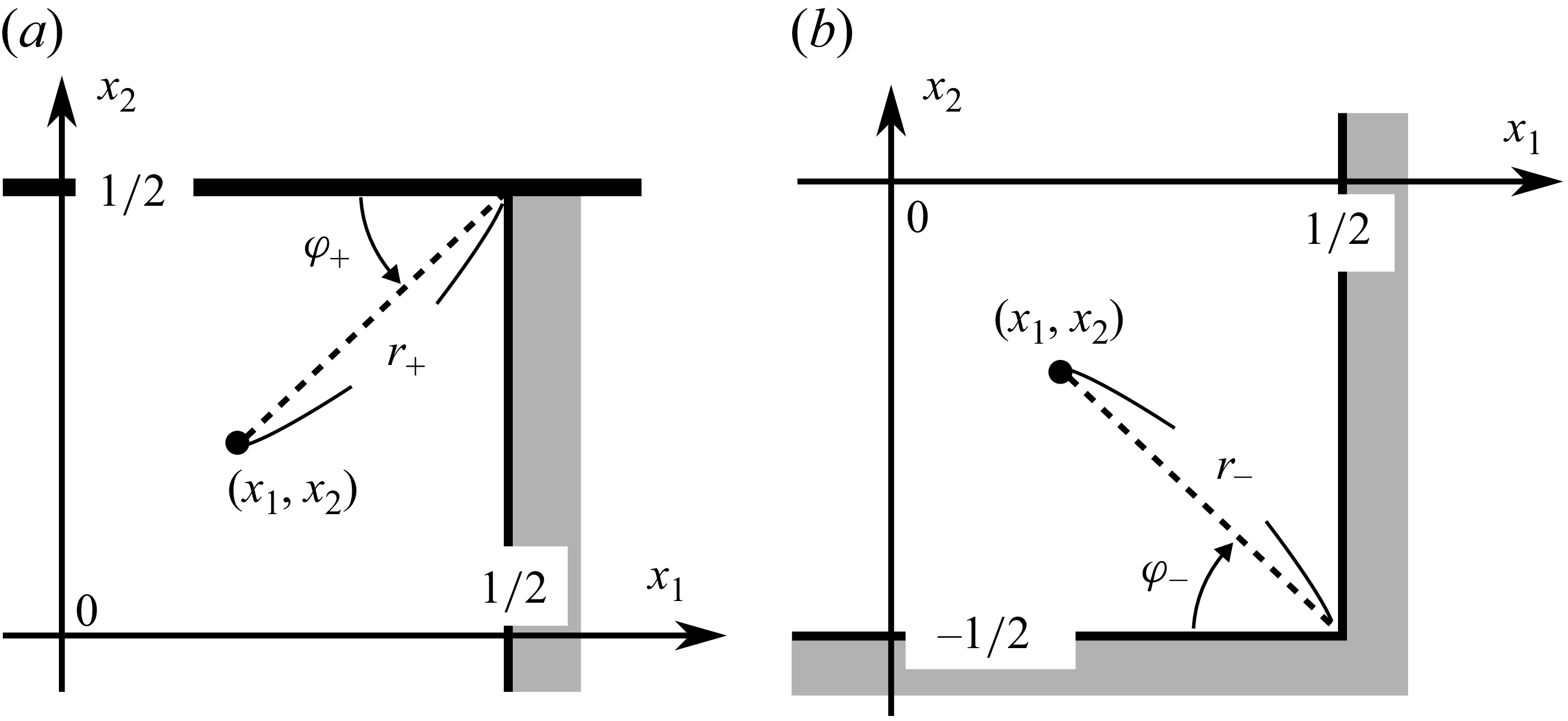
 r+
 φ+
 r−
 φ−

 k=0.01
 k=1
 k=10
 (u1/uw,u2/uw)
 (±1/2,±1/2)
 (0,0.15)
 (0,0)
 (0.1,−0.1)
 (0.2,−0.2)
 (0.3,−0.3)
 (0.4,−0.4)
 (0.45,−0.45)
 (0.49,−0.49)
 (−0.49,−0.49)

 P12/uw
 P11/uw
 P22/uw
 P/uw
 x1x2
 k=0.01
 k=1
 k=10
 0.15
 0.1
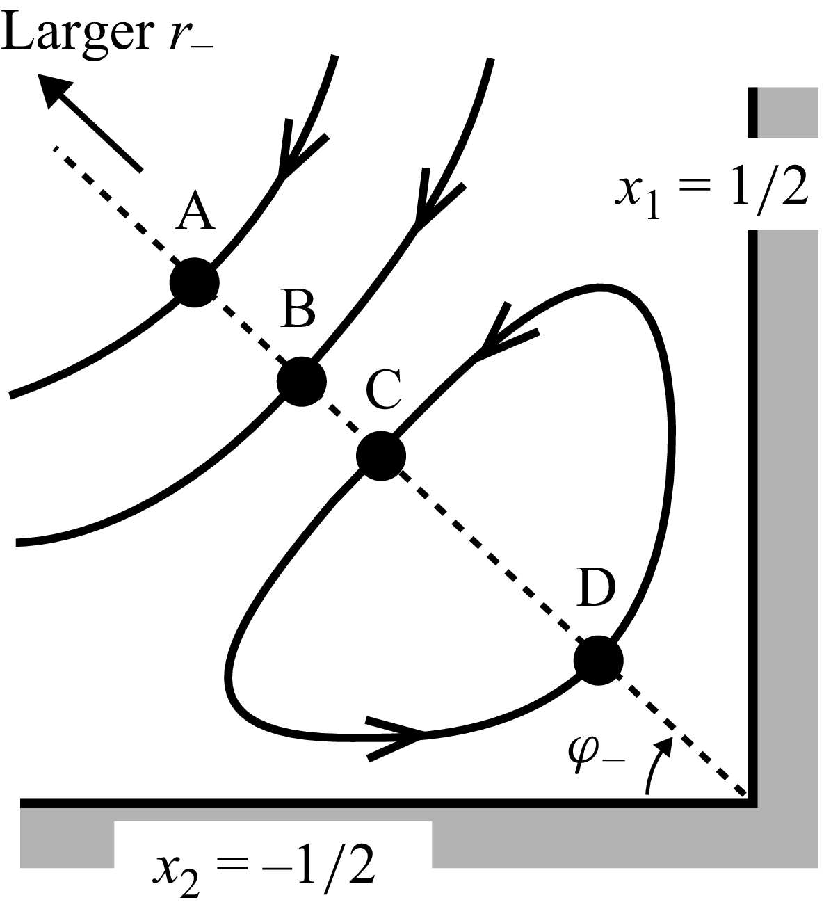
 (1/2,−1/2)
 φ−
 r−
 uφ−

 (1/2,−1/2)
 φ−=π/4
 uφ−/uw
 r−
 0
 0
 0
 0
 k

 (1/2,−1/2)
 k
 0.4≤x1≤0.5
 −0.5≤x2≤−0.4
 0.494≤x1≤0.5
 −0.5≤x2≤−0.494
 k
 0.03
 0.02
 0.01
 0.002
 0.0015
 0.001
 0.0006
 0.0003
 (m,−m)
 m=0.42
 0.4325
 0.445
 0.448
 0.468
 0.475
 0.485
 0.495
 0.4975
 0.4977
 (m,−m)
 m=0.495
 0.4957
 0.4964
 0.4972
 0.4986
 0.4994
 0.4999

 k=0.01
 u1/uw
 u2/uw
 P12/uw
 φ+
 r+
 (1/2,1/2)
 r+=0.2025
 0.02260
 2.771×10⁻³
 2.770×10⁻⁴
 2.778×10⁻⁵
 r+→0
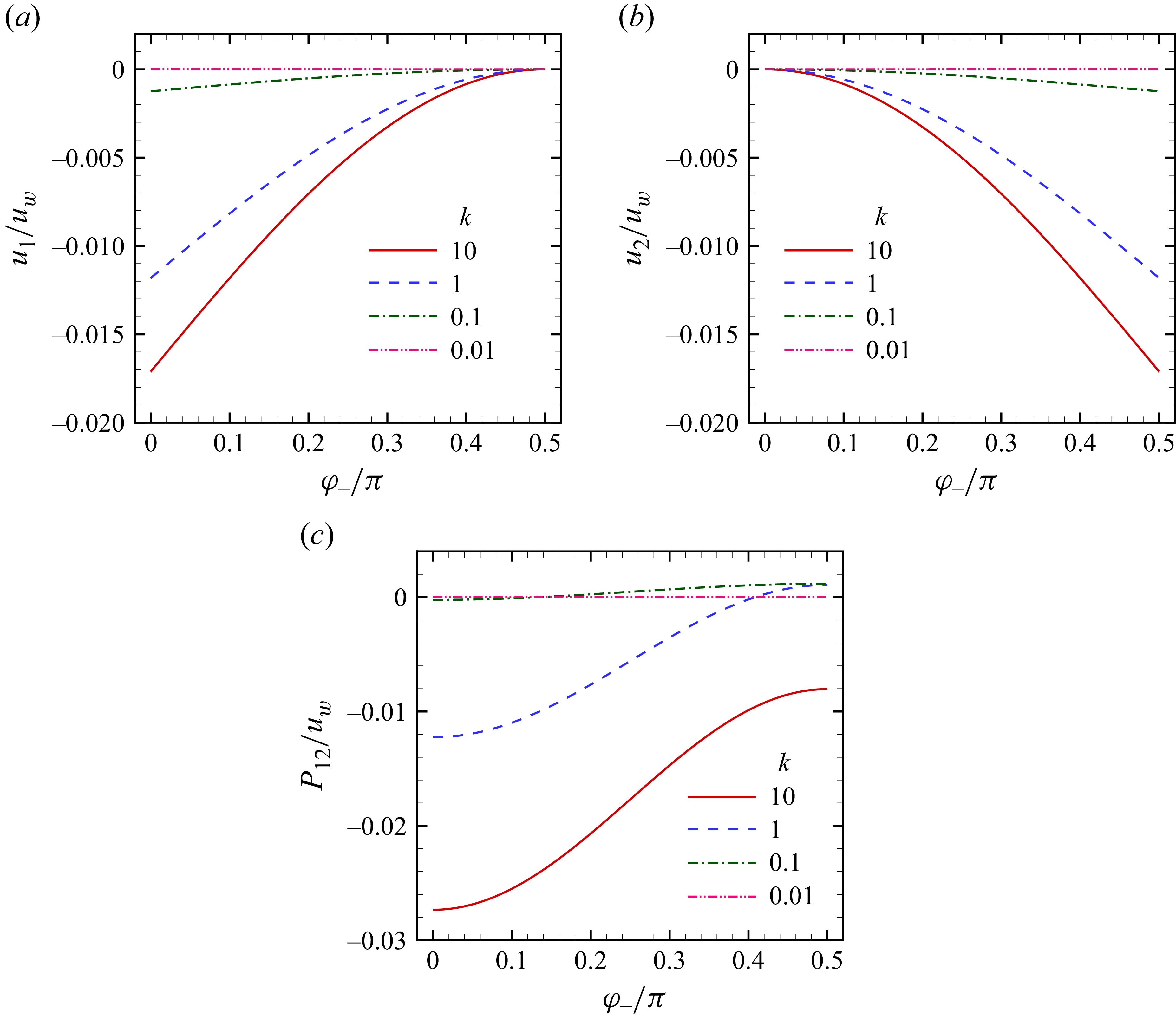
 r−→0
 u1/uw
 u2/uw
 P12/uw
 φ−

 (1/2,1/2)
 k=0.01
 (0.46,0.46)
 (0.47,0.47)
 (0.48,0.48)
 (0.49,0.49)
 (0.496,0.496)
 0.1
 |u|/uw

 P12/uw
 P11/uw
 P22/uw
 P/uw
 (1/2,1/2)
 k=0.01
 0.1
 0.2

 k=0.1
 0.01
 0.001
 u1/uw
 φ+=0
 u2/uw
 φ+=π/2
 P12/uw
 φ+=0
 P12/uw
 φ+=π/2
 r+
 (1/2,1/2)

 x1
 k=0.03
 0.01
 0.003
 0.001
 0.0003
 u1/uw
 P12/uw
 φ+=0
 r+/k
 (1/2,1/2)
 u1/uw
 P12/uw
 ((1/2−x1)/k,(1/2−x2)/k)
 k
 0.1
 0.05

 F1U
 F1B
 F1R−1
 F2R
 k
 −F1U/uw
 −F1B/uw
 (F1R−1)/uw
 −F2R/uw
 −F1U/uw
 −F1B/uw
 (F1R−1)/uw
 −F2R/uw
 −F1U/uwk
 −F1B/uwk
 (F1R−1)/uwk
 −F2R/uwk
 (−F1U/uw,−F1B/uw,(F1R−1)/uw,−F2R/uw)|k→∞=(0.68533,0.005235,0.34528,0.18723)

 P12/uw
 r+
 (1/2,1/2)
 P12/uw
 P/uw
 r+/k

 x
 φ+
 ℓ
 (ζ1,ζ2)
 θ
 x−dℓ
 n
 ζ1
 ζ2
 ζ1>0
 ζ2<0
 (1/2−0,−1/2)
 (1/2,−1/2+0)



