





1. Introduction
Debris-covered glaciers have their lower ablation zone mantled by a layer of rock debris, ranging from fine sediment to large boulders, that has fallen or been transported onto the ice surface (Scherler and others, Reference Scherler, Wulf and Gorelick2018; Mayr and Hagg, Reference Mayr, Hagg, Heckmann and Morche2019; Pellicciotti and others, Reference Pellicciotti2026). They are commonly found in tectonically active mountain ranges such as the Himalayas, Alaska and the Andes, where steep topography and high erosion rates promote intense sediment supply (Scherler and others, Reference Scherler, Wulf and Gorelick2018; Herreid and Pellicciotti, Reference Herreid and Pellicciotti2020). Debris input from avalanches and rockfalls in the accumulation zone is incorporated into the glacier ice and subsequently transported downglacier, where it re-emerges and concentrates at the surface within the ablation zone due to ice flow and melt (Anderson and Anderson, Reference Anderson and Anderson2016; Reference Anderson and Anderson2018). Additionally, significant amounts of material may also be delivered directly to the ablation zone from valley walls and degrading moraines (Rowan and others, Reference Rowan, Egholm, Quincey and Glasser2015; Anderson and Anderson, Reference Anderson and Anderson2018). The extent and thickness of debris on a glacier surface is thus the result of a combination of erosion rates, tectonic activity, and glacier mass balance and dynamics (Mayr and Hagg, Reference Mayr, Hagg, Heckmann and Morche2019; Compagno and others, Reference Compagno2022; Kirkbride and others, Reference Kirkbride2023).
Although debris-covered ice accounts for only about 7% of the global mountain glacier area (Scherler and others, Reference Scherler, Wulf and Gorelick2018; Herreid and Pellicciotti, Reference Herreid and Pellicciotti2020), it is widely but heterogeneously distributed, with hotspots in Alaska, the Karakoram and the Himalayas (Scherler and others, Reference Scherler, Wulf and Gorelick2018; Herreid and Pellicciotti, Reference Herreid and Pellicciotti2020). In the Southern Andes, debris-covered ice covers more than 2130 km2 (Scherler and others, Reference Scherler, Wulf and Gorelick2018). The Central Andes of Argentina and Chile (hereafter Central Andes; 30 $^\circ$–37
 $^\circ$ S) represent the main concentration area, where debris covers 40% of the glacierised area within the Atlantic basins (Scherler and others, Reference Scherler, Wulf and Gorelick2018; Zalazar and others, Reference Zalazar2020). Despite their regional abundance, debris-covered glaciers in the Central Andes remain poorly understood (Masiokas and others, Reference Masiokas2020; Fontrodona-Bach and others, Reference Fontrodona-Bach2025; Pellicciotti and others, Reference Pellicciotti2026), leaving significant gaps in understanding their spatial evolution and the physical processes governing interactions between debris and ice.
Overall, glaciers around the globe are currently out of balance and losing mass at accelerating rates (Hugonnet and others, Reference Hugonnet2021; Dussaillant and others, Reference Dussaillant2025; GlaMBIE Team, 2025). In addition, a steady increase in debris-covered area has been reported across several mountain ranges worldwide (Glasser and others, Reference Glasser, Holt, Evans, Davies, Pelto and Harrison2016; Herreid and Pellicciotti, Reference Herreid and Pellicciotti2020; Falaschi and others, Reference Falaschi2021; Fleischer and others, Reference Fleischer, Otto, Junker and Hölbling2021; Compagno and others, Reference Compagno2022; McCarthy and others, Reference McCarthy, Miles, Kneib, Buri, Fugger and Pellicciotti2022a). The evolution of the debris layer plays a key role in the response of debris-covered glaciers to climate forcing, influencing glacier mass balance and driving changes in ablation rates, glacier dynamics, geometry and runoff contribution (Anderson and others, Reference Anderson, Armstrong, Anderson, Scherler and Petersen2021; Racoviteanu and others, Reference Racoviteanu, Nicholson, Glasser, Miles, Harrison and Reynolds2022). In recent literature, glacier ice not covered by supraglacial debris is referred to as either ‘debris-free’ (Banerjee and Shankar, Reference Banerjee and Shankar2013; Ferri and others, Reference Ferri2020; Fontrodona-Bach and others, Reference Fontrodona-Bach2025) or ‘clean’ (Fyffe and others, Reference Fyffe2014; Shea and others, Reference Shea, Kraaijenbrink, Immerzeel and Brun2021; Feroz and others, Reference Feroz, Liang, Li, Li, Rahman and Yang2025), both terms are equivalent, and we adopt the former throughout.
Depending on the thickness of the debris layer, supraglacial debris can increase or decrease ablation (Østrem, Reference Østrem1959). When the debris layer is thin ( $ \lt $2 cm, approximately), ablation rates increase relative to debris-free ice because the reduced surface albedo enhances the absorption of solar radiation (Østrem, Reference Østrem1959; Cuffey and Paterson, Reference Cuffey and Paterson2010; Reid and Brock, Reference Reid and Brock2010; Reznichenko and others, Reference Reznichenko, Davies, Shulmeister and McSaveney2010; Collier and others, Reference Collier, Maussion, Nicholson, Mölg, Immerzeel and Bush2015; Pellicciotti and others, Reference Pellicciotti2026). In contrast, thicker debris layers progressively reduce melt rates by insulating the ice from atmospheric conditions (Scherler and others, Reference Scherler, Wulf and Gorelick2018; Anderson and others, Reference Anderson, Armstrong, Anderson, Scherler and Petersen2021; Huo and others, Reference Huo, Bishop and Bush2021a). Globally, supraglacial debris is thought to reduce ablation by
 $\sim$37% (Rounce and others, Reference Rounce2021). Surface features such as ice cliffs and ponds, however, can locally disrupt the insulating effect, acting as melting hotspots and enhancing overall mass loss at both local and glacier-wide scales (Han and others, Reference Han, Wang, Wei and Liu2010; Brun and others, Reference Brun2018; Buri and Pellicciotti, Reference Buri and Pellicciotti2018; Anderson and others, Reference Anderson, Armstrong, Anderson, Scherler and Petersen2021).
Despite the insulating effect of debris, debris-covered glaciers may lose mass at rates comparable to debris-free glaciers, a phenomenon known as the debris-cover anomaly (Kääb and others, Reference Kääb, Berthier, Nuth, Gardelle and Arnaud2012; Pellicciotti and others, Reference Pellicciotti, Stephan, Miles, Herreid, Immerzeel and Bolch2015). This apparent contradiction is best explained by a combination of interacting processes. Supraglacial ice cliffs and ponds act as localised ablation hotspots, contributing up to 17–26% of total melt from debris-covered ice (Brun and others, Reference Brun2018; Buri and others, Reference Buri, Miles, Steiner, Ragettli and Pellicciotti2021; Sato and others, Reference Sato2025). In addition, glacier dynamics can sustain thinning even where thick debris suppresses local melt. Numerical modelling shows that temporal changes in emergence and submergence velocities redistribute mass along glacier tongues, producing dynamic thinning that can maintain or even enhance surface lowering despite reduced sub-debris ablation (Banerjee, Reference Banerjee2017).
In the Central Andes, debris-covered and debris-free glaciers can contribute similarly to runoff in some basins (e.g.
Ayala and others, Reference Ayala2016). However, the influence of supraglacial debris on glacier melt and hydrological response remains uncertain at regional scales, as studies report contrasting behaviour when moving beyond individual basin analyses (e.g.
Burger and others, Reference Burger2019). Monitoring glacier change is particularly critical in the Central Andes of Argentina, where  $\sim$2.8 million people and key socio-productive activities depend on streamflow fed by snow and glaciers (INDEC, 2023). Although glacier mass balance was generally stable during 2000–09, the region has experienced widespread mass loss since then due to major droughts (Dussaillant and others, Reference Dussaillant2019; Ferri and others, Reference Ferri2020). During drought years, glaciers become the primary water source for downstream communities (e.g.
Ayala and others, Reference Ayala, Farías-Barahona, Huss, Pellicciotti, McPhee and Farinotti2020; Crespo and others, Reference Crespo, Fernandoy, Cara, Klarian and Lavergne2020; McCarthy and others, Reference McCarthy2022b; Toum and others, Reference Toum, Villalba and Masiokas2025). Mass loss rates also vary with debris cover, with less debris-covered glaciers showing greater losses (Ferri and others, Reference Ferri2020).
Systematic monitoring of surface characteristics is essential to better understand the mass balance of debris-covered glaciers (e.g. Gardelle and others, Reference Gardelle, Berthier and Arnaud2012; Vincent and others, Reference Vincent2016; Brun and others, Reference Brun2018; Shea and others, Reference Shea, Kraaijenbrink, Immerzeel and Brun2021). The complex interaction between debris cover and melt processes complicates the integration of supraglacial debris into glacier models, limiting the reliability of long-term projections of glacier evolution (Compagno and others, Reference Compagno2022; Pellicciotti and others, Reference Pellicciotti2026). Classification algorithms that identify glacier facies (such as ice, snow and debris) are widely used to assess glacier change across mountain regions (e.g. Racoviteanu and others, Reference Racoviteanu, Rittger and Armstrong2019; Rastner and others, Reference Rastner2019; Falaschi and others, Reference Falaschi2021; Mitkari and others, Reference Mitkari, Arora, Tiwari, Sofat, Gusain and Tiwari2022; Thomas and others, Reference Thomas, Robson and Racoviteanu2023; Tielidze and others, Reference Tielidze, Iacob and Holobâcă2024; Feroz and others, Reference Feroz, Liang, Li, Li, Rahman and Yang2025; Loibl and others, Reference Loibl, Richter and Grünberg2025). Advances in remote sensing have strengthened these automated approaches, particularly in regions with limited observational data such as the Andes (Rabatel and others, Reference Rabatel2012), where publicly available tools are essential for ensuring reproducibility and addressing persistent knowledge gaps.
Metrics derived from remote sensing provide effective proxies for glacier state and evolution. Snowline altitude (SLA) and snow-cover ratio (SCR) at the end of summer are commonly used as proxies for equilibrium-line altitude (ELA) and accumulation-area ratio (AAR), as they capture the transition between accumulation and ablation zones near the end of the hydrological year (e.g. Cuffey and Paterson, Reference Cuffey and Paterson2010; Shukla and Qadir, Reference Shukla and Qadir2016; Herreid and Pellicciotti, Reference Herreid and Pellicciotti2020). These metrics can be efficiently retrieved from satellite data to monitor glacier mass balance (e.g. Racoviteanu and others, Reference Racoviteanu, Rittger and Armstrong2019; Rastner and others, Reference Rastner2019; Podgórski and others, Reference Podgórski, Pętlicki, Fernández, Urrutia and Kinnard2023). For debris-covered glaciers, additional metrics such as debris-area ratio (DAR) and debris-emergence elevation (DEE) provide further insight into glacier evolution. Upward shifts in DEE can indicate glacier sensitivity to warming and negative mass-balance conditions (Shea and others, Reference Shea, Kraaijenbrink, Immerzeel and Brun2021), especially under reduced seasonal snow cover, an increasingly common condition in the Central Andes (Farías-Barahona and others, Reference Farías-Barahona2019; Pitte and others, Reference Pitte2022).
In this study, we analyse the evolution of surface characteristics in 229 debris-covered glaciers in the Central Andes of Argentina over four decades (1985–2024). Building on the Automated Snow Mapping on Glaciers (ASMAG) classification framework applied to Landsat TM, ETM+, OLI and Sentinel-2 imagery (Rastner and others, Reference Rastner2019; Zeller, Reference Zeller2020), we implemented an enhanced Python-based algorithm (hereafter ANDESMAG) that integrates snow-related (SLA, SCR) and debris-related (DAR, DEE) metrics. We validated the automated classification of debris-free and debris-covered glacier areas using the National Glacier Inventory of Argentina (NGI; Zalazar and others, Reference Zalazar2020). Moreover, we examined the links between the glacier metrics and observational climate records to assess their consistency with regional climate variability using the ERA5-Land reanalysis. Thereby, we provide new insights into debris-covered glaciers in a region with limited long-term observations, contributing to a broader understanding of Andean glacier response to climate influences.
2. Study area
The Central Andes (30 $^\circ$–37
 $^\circ$ S) comprise the highest sector of the Andes (Lliboutry, Reference Lliboutry, Williams and Ferrigno1998), with several peaks above 6000 m a.s.l., including Aconcagua (6961 m a.s.l.), the highest mountain in the Southern and Western Hemispheres. High tectonic activity, steep relief and broad thermal amplitude contribute to the substantial input of rocky debris from headwalls and valley sides onto glacier surfaces. This region is also among the most glacierised in South America, containing 8076 glaciers and other cryospheric landforms in Argentina, including debris-free and debris-covered glaciers, perennial snowfields and rock glaciers (Fig. 1a). The Central Andes of Argentina also contain 82% of the country’s debris-covered ice area and rank second in total glacierised area after the Southern Patagonian Andes (Zalazar and others, Reference Zalazar2020).
Glaciers in the Central Andes of Argentina are distributed across seven major Atlantic basins: San Juan, Mendoza, Tunuyán, Diamante, Atuel, Llancanelo and Colorado, from north to south. These basins span a pronounced altitudinal gradient, with average glacier elevation ranging from about 2600 m a.s.l. in the south to over 6800 m a.s.l. in the north (Fig. 1d). Glacierised area is unevenly distributed among the basins, with the sum of the Mendoza (570 km2), San Juan (509 km2) and Tunuyán (407 km2) basins accounting for approximately 85% of the region’s total. Although most glaciers are small (less than 2 km2), a few large debris-covered valley glaciers exceeding 10 km2 account for most of the total ice area (Fig. 1c).
Glacier distribution in the Central Andes of Argentina. (a) Map of glacier distribution across the five main basins, highlighting the type of glaciers and the debris-covered percentage. (b) Mean aspect of glacier type in the Central Andes (normalised by number). (c) Area (colour bars) and number (unfilled bars) of glaciers by type in the Central Andes. (d) Altitudinal distribution of glaciers as a function of latitude, the grey line representing the elevation profile of the Andes; bubble size indicates the area of each individual glacier. Glacier information from the NGI (Zalazar and others, Reference Zalazar2020), and elevation data from the SRTM-V4 DEM. Base map: Esri World Topographic Map.

1 Long description
Panel a covers 30 to 37 degrees south along the Chile–Argentina border. The five study basins are labelled San Juan, Mendoza, Tunuyán, Diamante and Atuel, with Llancanelo and Colorado also named to the south. An inset locates the area in southern South America. Light blue marks perennial snowfields, green debris–free glaciers, grey rock glaciers, and yellow, orange and black debris-covered glaciers with 5 to 50, 50 to 90 and more than 90 per cent debris cover. Glaciers cluster between 31 and 35 degrees south. Panel b has a radial axis to 0.40 and one line per glacier type, all peaking between south and south–east. Panel c shows counts to about 5400 and areas to about 560 square kilometres, largest for debris–covered glaciers with 5 to 50 per cent cover. Panel d plots altitude from 3000 to 7000 metres against latitude from 37 to 30 degrees south, with glaciers sitting progressively higher towards the north.
The regional ELA is highly variable, typically ranging from  $\sim$2500 to 4500 m a.s.l. from south to north, depending on the topographic setting (Condom and others, Reference Condom, Coudrain, Sicart and Théry2007; Ferri and others, Reference Ferri2020). On average, debris-covered glaciers occur at slightly lower elevations (
 $\sim$4300 m a.s.l.) compared to debris-free glaciers (
 $\sim$4500 m a.s.l.) (Ferri and others, Reference Ferri2020; Zalazar and others, Reference Zalazar2020).
In terms of climate setting, the Central Andes region is characterised by a semi-arid to arid climate with pronounced seasonality in precipitation. Most snowfall occurs during the austral winter (April–October) and is associated with frontal systems and atmospheric rivers transporting moisture from the Pacific Ocean (Viale and Nuñez, Reference Viale and Nuñez2011; Rivera and others, Reference Rivera, Otta, Lauro and Zazulie2021). Summer precipitation is scarce and predominantly convective (Viale and Garreaud, Reference Viale and Garreaud2015; Benedicto and others, Reference Benedicto, Viale and Salio2025). Climatic conditions vary markedly with latitude. Glaciers between 30 $^\circ$ and 31
 $^\circ$ S experience relatively low annual precipitation (
 $\sim$300 mm), evenly distributed throughout the year, along with some of the coldest mean annual temperatures in the Andes (around
 $-$4.5
 $^\circ$C). Southward, from 32
 $^\circ$ to 37
 $^\circ$ S, glaciers are exposed to higher annual precipitation (
 $\sim$700 mm), predominantly falling during winter months, and to milder mean annual temperatures approaching 0
 $^\circ$C (Sagredo and Lowell, Reference Sagredo and Lowell2012). Since 2009, this region has been affected by the Central Andes Megadrought, an unprecedented period of severe precipitation deficit (30–50% below the 20th-century average) and sustained atmospheric dryness that extends between 30
 $^\circ$ and 38
 $^\circ$ S, and which represents the most severe and prolonged drought recorded in the instrumental period for this part of the Andes (Garreaud and others, Reference Garreaud, Boisier, Rondanelli, Montecinos, Sepúlveda and Veloso-Aguila2020; Rivera and others, Reference Rivera, Otta, Lauro and Zazulie2021).
3. Material and methods
3.1. Data sources
3.1.1. Optical imagery and DEM
We used satellite images from the Landsat TM, ETM+, OLI and Sentinel-2 top-of-atmosphere collections obtained through Google Earth Engine (Gorelick and others, Reference Gorelick, Hancher, Dixon, Ilyushchenko, Thau and Moore2017). We opted for this processing level to omit atmospheric corrections to avoid variability between individual scenes and errors associated with corrections of short spectral bands (Chander and others, Reference Chander, Markham and Helder2009; Teixeira Pinto and others, Reference Teixeira Pinto, Jing and Leigh2020; Zeller, Reference Zeller2020). We focused on the late ablation season in the Southern Hemisphere (days of year 40–120), when snow cover typically reaches the annual minimum in the Central Andes. We processed more than 60 000 image tiles, excluding partially covered scenes to avoid data gaps. For each year, the image with the least snow cover was selected for each glacier (Fig. S13).
To calculate altitudinal metrics (DEE and SLA) and topographic shading (Section 3.2.1), we used the SRTM-V4 DEM (Jarvis and others, Reference Jarvis, Reuter, Nelson and Guevara2008) available via Google Earth Engine. This choice is supported by the thinning rates reported for the region:  $-0.31\pm0.19$ m w.e. a–1 (Dussaillant and others, Reference Dussaillant2019) and
 $-0.36\pm0.19$ m w.e. a–1 (Ferri and others, Reference Ferri2020) for the Central Andes over 2000–18, implying surface elevation changes well within the uncertainty of our altitudinal metrics (91–99 m; Section 3.5). We acknowledge this limitation and note that ANDESMAG supports time-varying DEMs as higher-quality products become available for the region (Section 5.5).
3.1.2. Glacier outlines
We used fixed outlines for each glacier based on the most recent version of the NGI (Zalazar and others, Reference Zalazar2020). The NGI was produced using supervised classification and additional manual corrections, with debris-covered areas delineated through visual interpretation. Glacier surfaces were mapped as separate polygons (e.g. debris-free, debris-covered), so a single glacier (NGI ID) may include multiple surface types as different polygons. Glaciers with at least 5% of their total area covered by debris were considered debris-covered; fully debris-free glaciers were excluded.
In total, we analysed 229 debris-covered glaciers (Table S1) covering 843 km2, which corresponds to approximately 74% of the total glacier area in the Central Andes of Argentina as reported in the NGI. More than 70% of the analysed glaciers are smaller than 3.5 km2. Most of the ice area is concentrated in a few large glaciers, with merely 30 glaciers accounting for more than 402 km2. Most of these glaciers are located within the Mendoza (93 glaciers, 339 km2), Tunuyán (56 glaciers, 268 km2) and San Juan (47 glaciers, 150 km2) basins, which are the most glacierised (Ferri and others, Reference Ferri2020). The Atuel and Diamante basins host 23 (62 km2) and 10 (24 km2) glaciers, respectively. Over 75% of the individual glacier metrics assessed in this study span 35 years or more within the full analysed period (1985–2024).
Glacier outlines from the NGI (2009–11 period) were used as fixed spatial masks for all surface classifications (Section 3.2.1), meaning that changes in glacier geometry thereafter are not captured in our analyses. When a glacier retreats, its DAR can increase even if the absolute debris-covered area is unchanged, as the debris-free area is preferentially lost. To quantify this effect, we conducted a fixed-outline error analysis (Section 5.5) on a stratified random sample of 30 glaciers (10 per class of initial debris coverage: low, 5–10%; intermediate, 10–50%; high, 50–90%). The fixed-outline error in DAR change is defined as the difference between DAR change computed using fixed NGI outlines and that computed using updated outlines, assuming an upper-bound scenario in which all glacier area lost since the NGI inventory is debris-free but remains classified as debris-covered area within the fixed glacier mask.
3.2. Automated classification algorithm (ANDESMAG)
We applied ANDESMAG, an implementation of the ASMAG algorithm in Python that uses Google Earth Engine (Gorelick and others, Reference Gorelick, Hancher, Dixon, Ilyushchenko, Thau and Moore2017) as a cloud-computing backend (Fig. 2), to derive DAR, DEE, SCR and SLA (Rastner and others, Reference Rastner2019; Zeller, Reference Zeller2020). This architecture enables efficient data handling and overcomes local computational limitations. ASMAG provides a robust tool for monitoring glacier surface characteristics, including metrics such as SCR and SLA, with reported accuracies of 82–92% for glacier facies and 91% for SLA (Rastner and others, Reference Rastner2019; Falaschi and others, Reference Falaschi2021). Its straightforward logic, global data availability, and open-access implementation enable easy integration of additional functionalities, facilitating its application in regions with limited observational data such as the Andes (Masiokas and others, Reference Masiokas2020; Falaschi and others, Reference Falaschi2021). To extend the applicability of ASMAG to debris-covered glaciers, we complemented the standard snow-related metrics (SLA, SCR) with debris-related metrics (DAR, DEE).
3.2.1. Glacier surface classification
The ANDESMAG core classification remains automated and consistent with earlier versions of ASMAG (Rastner and others, Reference Rastner2019; Zeller, Reference Zeller2020; Falaschi and others, Reference Falaschi2021). Sensor differences across Landsat (TM, ETM+ and OLI) and Sentinel-2 were harmonised in pre-processing: bands were renamed to a common scheme, Sentinel-2 reflectance was rescaled to the 0–1 range of the Landsat top-of-atmosphere products, and solar geometry and quality flag metadata were parsed per sensor. The same decision-tree classifier is then applied to all sensors, combining topographic criteria, spectral indices and reflectance thresholds in the visible, near-infrared and shortwave-infrared bands to separate snow, ice, debris, clouds and shadowed areas at 30 m resolution within the glacier mask (Supplementary Material Section 10 provides an overview of thresholds applied at different processing steps; Fig. S12).
Before classification, a cloud filter was applied by computing a cloud score within each glacier area. Cloud detection was based on the high reflectance of clouds in visible, near-infrared and shortwave-infrared bands. To reduce confusion between snow and clouds, the NDSI (Hall and Riggs, Reference Hall, Riggs, Singh, Singh and Haritashya2011) was also considered. In this study, images with a cloud score exceeding 10% of the glacier area were excluded. To reduce illumination effects in steep terrain, we applied a topographic correction following Ekstrand (Reference Ekstrand1996), as implemented in Rastner and others (Reference Rastner2019).
Cloud shadows were estimated by projecting cloud masks using solar azimuth and elevation. The projected mask was spectrally refined by identifying dark pixels in the near-infrared and shortwave-infrared bands to better isolate true shadowed areas. Topographic shadows were additionally derived from the SRTM-V4 DEM based on slope, aspect and solar geometry. The two masks were then merged and excluded from the classification.
ANDESMAG classifies glacier surface facies (snow, ice and debris) on a pixel basis within glacier masks free of clouds and shadows, using combined spectral criteria. Debris cover is identified from low NDSI values and high shortwave-infrared reflectance. Snow detection is performed in two steps: bright snow is first identified from high NDSI values, and snow and bare ice are then separated within debris-free glacier areas using the Otsu method applied to the near-infrared reflectance histogram of each scene (Otsu, Reference Otsu1979). Thresholds derived using the Otsu method are constrained to a predefined range to ensure robust performance. This approach, which adapts to each scene, provides a separation between bright snow and darker ice and has been widely used in optical snow mapping (e.g. Yin and others, Reference Yin, Cao, Chen, Shao and Chen2013; Rastner and others, Reference Rastner2019; Sun and others, Reference Sun, Li, Tan, Gao, Wang and Xiong2025).
Workflow for generating facies maps and the database of monitored metrics. Landsat and Sentinel-2 images are queried and filtered (pre-processing) through a local server using the Google Earth Engine API for Python. These images are then classified pixel-by-pixel (processing), and finally, monitoring metrics are extracted (post-processing). The resulting data can be stored either in the cloud or on the local server (adapted from Zeller, Reference Zeller2020).

Figure 2 Long description
The local server block contains a user input box holding the evaluation period, and two database cylinders for facies maps and monitoring metrics. An arrow carries the user input into the cloud block. In the pre-processing stage, four cylinders hold glacier outlines, Landsat 5, 7 and 8 imagery, Sentinel-2 imagery and the SRTM version 4 digital elevation model. Their outputs converge on the processing stage, where a classifier produces a stack of classified images. These feed the post-processing stage, where a single box extracts the monitoring metrics. Two return arrows run from the classified images and from the extracted metrics back to the facies maps and monitoring metrics cylinders on the local server.
3.2.2. Glacier metrics
We derived four annual metrics to characterise glacier surface changes, namely DAR, DEE, SCR and SLA (Fig. 3). SCR and DAR were computed as the portion of glacier area classified as snow and debris, respectively (Fig. 3b). SLA and DEE were extracted with the main-patch method (Rastner and others, Reference Rastner2019; Zeller, Reference Zeller2020), defined by the transition between the largest contiguous facies (snow–ice for SLA, debris–ice for DEE; Fig. 3b). In both cases, we used the median elevation of contact pixels to reduce the influence of outliers and local topographic variability.
Example of image classification and glacier metric extraction for Alto del Plomo glacier (ID: G700069O329897S). (a) Landsat OLI false-colour composite (near-infrared, red, green) from February 2019. (b) Classified map showing snow, ice and debris-covered ice. The pink and yellow lines highlight contact zones between snow and ice and between ice and debris, respectively, used to derive the SLA and the DEE. Base map: Esri World Topographic Map.

Figure 3 Long description
The glacier runs north to south, with a wide upper basin and a narrow tongue about 6 kilometres long. In the left panel the surface is pale grey and blue in the upper basin and dark brown along the tongue, against pale shaded relief. In the right panel blue marks ice, cyan marks snow and orange marks debris. Snow occupies the upper basin, ice covers most of the glacier, and debris forms a band along both margins that widens downglacier until it covers the whole terminus. A pink line across the upper basin is labelled SLA and a yellow line across the middle of the tongue is labelled DEE. Scale bars span 2 kilometres.
We tested data normality using the Shapiro–Wilk test (Wilks, Reference Wilks2011). Temporal trends were then evaluated with linear regression and the Mann–Kendall test (Yue and Wang, Reference Yue and Wang2002), which is suitable for detecting monotonic trends in time series. To assess whether glacier metrics underwent a significant shift following the onset of the Megadrought, the most severe drought recorded in the instrumental period for this region (Section 2;
Garreaud and others, Reference Garreaud, Boisier, Rondanelli, Montecinos, Sepúlveda and Veloso-Aguila2020; Rivera and others, Reference Rivera, Otta, Lauro and Zazulie2021), mean values before and after 2009 were compared using Welch’s  $t$-test (von Storch and Zwiers, Reference von Storch and Zwiers2002) for normally distributed data and the Mann–Whitney
 $U$ test (Wilks, Reference Wilks2011) otherwise. All statistical analyses were performed on annual series aggregated at both regional and basin scales, using a 95% confidence level for significance testing. We computed the change rate for each glacier metric using the Theil–Sen estimator (Hirsch and others, Reference Hirsch, Slack and Smith1982), a non-parametric method suitable for detecting trends in time series that may include outliers. Relationships between the change rates of each metric and glacier attributes (latitude, elevation, area, slope and aspect) were then examined using Spearman’s rank correlation (Wilks, Reference Wilks2011) to assess monotonic associations. Relationships among metrics were evaluated by computing Pearson correlation (
 $r$) and coefficients of determination (
 $R^{2}$) at both regional and basin scales, ensuring that all time series met the assumptions required by these tests (Helsel and Hirsch, Reference Helsel and Hirsch1993; Wilks, Reference Wilks2011).
3.3. Climate analysis
We used monthly air temperature and precipitation anomalies from the ERA5-Land reanalysis (Muñoz-Sabater and others, Reference Muñoz-Sabater2021) for 1985–2024, as continuous high-elevation meteorological records spanning this period are unavailable. Data were extracted from 0.1 $^\circ$ grid cells located within the bounding boxes of each basin and the full study region and spatially averaged within each domain. As these domains inevitably include unglacierised terrain, the resulting climate variables represent regional atmospheric forcing rather than meteorological conditions at the glacier scale.
To complement ERA5-Land, we added mean MODIS snow-cover area anomalies from the Observatorio de Nieve en los Andes de Argentina y Chile (Cara Ramirez and others, Reference Cara Ramirez, Masiokas, Viale and Villalba2016), an independent analogue to our SCR estimates at the basin rather than the glacier scale. We also included the 0 $^\circ$C isotherm altitude derived from daily radiosonde profiles at the Santo Domingo station in central Chile, corrected for a known geographic shift around 2000 (Figs S7 and S8). Anomalies for ERA5-Land and the 0
 $^\circ$C isotherm were computed relative to the 1980–2010 baseline. For MODIS snow-cover area, available only from 2000 onward, anomalies were calculated relative to the 2000–24 mean.
To assess glacier–climate relationships, we correlated each glacier metric (DAR, DEE, SCR, SLA) with ERA5-Land mean temperature and total precipitation over the hydrological year (1 May–30 April) using the Pearson correlation coefficient ( $r$). To account for temporal autocorrelation, significance was assessed using an effective sample size based on lag-1 autocorrelation (Bretherton and others, Reference Bretherton, Widmann, Dymnikov, Wallace and Bladé1999). Within each domain (the region and each basin), the Benjamini–Hochberg false-discovery rate (Benjamini and Hochberg, Reference Benjamini and Hochberg1995) controlled for multiple comparisons (eight tests; FDR-adjusted
 $p$, i.e.
 $q \lt $ 0.05). Associations that remained significant after linear detrending of both series were interpreted as robust interannual climate–glacier relationships.
3.4. Evaluation of ANDESMAG surface classification
We validated the classification of debris-free and debris-covered areas against NGI surface maps (Zalazar and others, Reference Zalazar2020). Produced by expert manual delineation, the NGI is the most reliable independent reference available in the region (Paul and others, Reference Paul2013). Because the NGI serves only to define the fixed glacier outlines, while the classification within them is produced independently by ANDESMAG, this validation evaluates surface type discrimination rather than glacier extent delineation.
We selected 49 glaciers from the Central Andes of different sizes (between 0.2 and 29 km2) with different percentages of debris cover (from 1% to 100%) (Table S2). For each glacier, we compared the NGI and ANDESMAG classifications on a pixel basis. Validation involved a confusion matrix to assess class agreement (debris-free versus debris-covered) and a regression analysis between DAR values from both sources. As the NGI does not distinguish between debris-free ice and seasonal snow (Zalazar and others, Reference Zalazar2020), both classes were merged into a single debris-free class. The validation assesses debris discrimination (and derived metrics such as DAR and DEE), but does not directly evaluate SLA or SCR. This simplification was necessary given the absence of independent glacier snow-cover datasets for the Central Andes, with the NGI representing the most robust reference currently available. The NGI was mapped from late-summer Landsat and ALOS (AVNIR-2, PRISM) imagery of 2009–11, and we matched our Landsat scenes to the NGI dates as closely as possible, with 93% within  $\pm$10 days (Fig. 8f).
3.5. Uncertainties and validation of glacier metrics
Uncertainty in the areal metrics DAR and SCR ( $e_{\mathrm{var,area}}$) was estimated from the combined effects of uncertainty in glacier outlines and uncertainty in facies classification. Glacier outline uncertainty (
 $e_{\mathrm{lim}}$) was set to 5%, following the NGI estimate reported by Zalazar and others (Reference Zalazar2020). Classification uncertainty (
 $e_{\mathrm{class}}$) was set to 6%, based on the validation of the facies maps (Section 3.4). Assuming independent errors, total uncertainty was obtained by propagation as follows:
 \begin{equation}
e_{\mathrm{var,area}} = \sqrt{e_{\mathrm{lim}}^{2} + e_{\mathrm{class}}^{2}}
\end{equation}
Uncertainty in the altitudinal metrics SLA and DEE ( $e_{\mathrm{var,altitude}}$) was estimated by combining the vertical uncertainty of the SRTM-V4 DEM and the uncertainty associated with ANDESMAG in applying the main-patch method to derive SLA and DEE. The DEM vertical uncertainty (
 $e_{\mathrm{dem}}$) was set to
 $\pm$23.5 m following Mukul and others (Reference Mukul, Srivastava, Jade and Mukul2017). Main-patch uncertainty (
 $e_{\mathrm{mp}}$) was estimated as the standard deviation of the elevation of the contact zone between snow and ice patches (for SLA) and between ice and debris patches (for DEE). Assuming independent errors, total uncertainty in the altitudinal metrics was calculated as follows:
 \begin{equation}
e_{\mathrm{var,altitude}} = \sqrt{e_{\mathrm{dem}}^{2} + e_{\mathrm{mp}}^{2}}
\end{equation}
To evaluate ANDESMAG performance, we compared the SLA and DEE outputs to SLA and DEE values derived from manual delineation (Figs S1 and S2). For SLA, automated estimates were compared with manually delineated snowlines from the same images ( $n$ = 31), following Rastner and others (Reference Rastner2019). An analogous analysis was performed for DEE using the NGI as reference (
 $n$ = 76). We assessed the effect of using fixed glacier outlines on DAR during the Megadrought period (Figs S3 and S4, Tables S6 and S7) by manually updating the outlines from 2009–11 to 2023–24 for 30 glaciers with varying debris-cover area. Further details are provided in Sections 5 and 6 of the Supplementary Material.
4. Results
4.1. Debris-covered glacier surface evolution
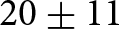
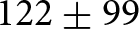
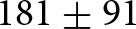
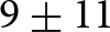
During the past four decades, debris-covered glaciers in the Central Andes have undergone a  $20\pm11$% increase in debris-covered area, a
 $122\pm99$ and
 $181\pm91$ m rise in DEE and SLA, and a
 $9\pm11$% decrease in SCR (Fig. 4). Debris-related metrics (DAR and DEE) showed the lowest interannual variability and statistically significant positive trends (
 $p \lt $ 0.001; Mann–Kendall), with regional slopes of 0.7% a–1 and 4 m a–1, respectively. In contrast, trends in snow-related metrics (SLA and SCR) were weaker and not statistically significant (
 $p$ = 0.099 and
 $p$ = 0.051, respectively). At the regional scale, DAR and DEE were strongly correlated (
 $r$ = 0.75,
 $R^{2}$ = 0.56), while DEE and SLA exhibited the highest association among all metrics (
 $r$ = 0.84,
 $R^{2}$ = 0.70; Fig. S9, Table S8).
Temporal evolution of glacier metrics for the 229 debris-covered glaciers over the past 40 years in the Central Andes. (a) DAR (%), (b) DEE (m a.s.l.), (c) SCR (%) and (d) SLA (m a.s.l.). Annual mean values across all studied glaciers are shown as dots, with vertical bars representing error. The solid lines represent a 5-year rolling mean, while the shaded areas indicate the 95% confidence interval. The Megadrought period (starting in 2009) is highlighted in grey.

Figure 4 Long description
Panel a plots DAR from 20 to 70 per cent in yellow and rises throughout, most steeply after 2009. Panel b plots DEE from 4200 to 4700 metres in dark yellow, peaks near 1997, falls to about 4350 metres near 2003 and rises to about 4470 metres by 2024. Panel c plots SCR from 0 to 60 per cent in light blue, holds near 25 per cent until about 2009 and then declines to about 10 per cent. Panel d plots SLA from 4400 to 5000 metres in teal, peaks near 1997, falls to about 4620 metres in the mid 2000s and rises to about 4790 metres by 2024. Dots scatter widely around the lines and the error bars are largest in the 1990s.
Debris-related metrics increased across all basins (Fig. 5). They increased at lower rates until the late 2000s, then accelerated with the onset of the Central Andes Megadrought. The Atuel basin recorded the largest increase in debris-covered area, with DAR increasing by  $44\pm11$% at a rate of 1.54% a–1 (Fig. 5e and f), while Tunuyán showed the smallest increase, reaching only
 $13\pm11$% at a rate of 0.6% a–1 (Fig. 5c and f). The DEE also increased significantly across all basins (
 $p \lt $ 0.01), with median elevation gains ranging from 57 m in Tunuyán (Fig. 5c and g) to a maximum of 211 m in Diamante (Fig. 5d and g). The post-2009 increases were significant in all basins (
 $p \lt $ 0.01;
 $t$-test or Mann–Whitney
 $U$). Across all basins, correlations between DAR and DEE were statistically significant (
 $r \gt $ 0.70,
 $R^{2} \gt $ 0.50), except in Tunuyán, where weaker but still significant relationships were observed (
 $r$ = 0.47,
 $R^{2}$ = 0.22; Figs S10 and S11).
Temporal evolution of debris-related metrics across Central Andes basins: San Juan (a), Mendoza (b), Tunuyán (c), Diamante (d) and Atuel (e). Solid gold and dashed brown lines denote 5-year rolling means of DAR (%) and DEE (m a.s.l.), respectively; shaded areas indicate 95% confidence intervals. Panels (f) and (g) show the distribution of changes in DAR and DEE across basins from 1985 to 2024.

Figure 5 Long description
In every basin both lines rise over the record, most steeply after about 2009. Axis ranges are 30 to 60 per cent and 4500 to 4800 metres in San Juan, 40 to 70 per cent and 4300 to 4600 metres in Mendoza, 10 to 55 per cent and 4000 to 4600 metres in Tunuyán, 10 to 70 per cent and 3400 to 4000 metres in Diamante, and 10 to 70 per cent and 3400 to 3650 metres in Atuel. Tunuyán is the most irregular, with a fall in the early 1990s and a step around 2009. The shaded bands are widest in Diamante and Tunuyán. Panel f runs from minus 75 to 75 per cent and shows boxes centred above zero in all basins, widest in Atuel and Diamante, with Tunuyán the closest to zero. Panel g runs from minus 500 to 750 metres and shows boxes centred above zero, with scattered outliers at both ends.
Snow-related metrics show widespread snow cover loss and rising snowlines at the end of summer across all basins of the Central Andes (Fig. 6). The strongest decrease in SCR occurred in the Atuel catchment (Fig. 6e and f), where it decreased by  $20\pm11$%, while Tunuyán (Fig. 6c and f) and Mendoza basins (Fig. 6b and f) showed moderate reductions below the level of uncertainty. Decreasing SCR trends were statistically significant in Atuel, Tunuyán and San Juan basins (
 $p \lt $ 0.05). Snowlines rose throughout the region, most in San Juan (
 $222\pm99$ m) and Atuel (
 $158\pm73$ m) and least in Tunuyán (
 $55\pm128$ m, within uncertainty); its trend was significant in all basins except Tunuyán (
 $p \gt $ 0.7). SCR and SLA were strongly and inversely correlated in all basins (
 $r$ =
 $-$0.72 to
 $-$0.95;
 $R^{2}$ = 0.51–0.91), and SLA also correlated with the debris-related metrics (generally
 $r \gt $ 0.6,
 $R^{2} \gt $ 0.4; Figs S10 and S11). Overall, associations were strongest in San Juan (
 $r \gt $ 0.85,
 $R^{2} \gt $ 0.70) and weakest in Tunuyán (
 $r \lt $ 0.57,
 $R^{2} \lt $ 0.30).
Temporal evolution of snow-related metrics across Central Andes basins: San Juan (a), Mendoza (b), Tunuyán (c), Diamante (d) and Atuel (e). Solid teal and dashed light blue lines denote 5-year rolling means of SLA (m a.s.l.) and SCR (%), respectively; shaded areas indicate 95% confidence intervals. Panels (f) and (g) show the distribution of changes in SCR and SLA across basins from 1985 to 2024.

Figure 6 Long description
In every basin the two lines diverge. SCR, on the left axis, falls over the record, most markedly after about 2009, while SLA, on the right axis, rises, most sharply after 2009. Axis ranges are 10 to 40 per cent and 4800 to 5200 metres in San Juan, 0 to 30 per cent and 4600 to 4900 metres in Mendoza, 0 to 60 per cent and 4200 to 5000 metres in Tunuyán, 0 to 60 per cent and 3600 to 4200 metres in Diamante, and 0 to 60 per cent and 3500 to 4000 metres in Atuel. The shaded bands are wide throughout and widest in Tunuyán and Diamante. Panel f runs from minus 50 to 75 per cent and shows boxes centred below zero in all basins, with numerous low outliers in Mendoza. Panel g runs from minus 1000 to 1500 metres and shows boxes centred above zero in all basins.
The analysis of individual glacier trends shows a spatial gradient in debris- and snow-related change rates driven by topographic and latitudinal factors (Fig. 7). The rate of DAR change (Fig. 7a) decreases markedly towards the north ( $\rho$ =
 $-$0.45,
 $p \lt $ 0.001) and with glacier length (
 $\rho$ =
 $-$0.10,
 $p$ = 0.002), while it increases with slope (
 $\rho$ = 0.22,
 $p \lt $ 0.001). DEE shows a weaker but significant negative correlation with latitude (
 $\rho$ =
 $-$0.13,
 $p \lt $ 0.001) and a positive correlation with glacier slope (
 $\rho$ = 0.23,
 $p \lt $ 0.001). In contrast, the SCR change rate increases towards lower latitudes (
 $\rho$ = 0.28,
 $p \lt $ 0.001) but declines with mean glacier elevation and area (
 $\rho$ =
 $-$0.40 and
 $-$0.36, respectively;
 $p \lt $ 0.001). The rate of SLA rise also increases with slope and glacier size (
 $\rho$ = 0.33–0.34,
 $p \lt $ 0.001) but decreases towards northern basins (
 $\rho$ =
 $-$0.32,
 $p \lt $ 0.001).
Altitudinal distribution of the glaciers studied as a function of latitude, with the grey line representing an elevation profile of the Andes; the size of the bubbles indicates the area of each glacier and the colour indicates the change rate of DAR in % a–1 (a), DEE in m a–1 (b), SCR in % a–1 (c) and SLA in m a–1 (d).

Figure 7 Long description
Each panel carries a key for bubble sizes of 1, 5 and 20 square kilometres. In panel a the colour scale runs from 0 to 2.0 per cent per year in pale yellow to gold, with the strongest values between 33 and 35 degrees south and below 5000 metres. In panel b the scale runs from 0 to 10.0 metres per year in pale yellow to brown, with values more widely scattered and the highest ones in the south and between 33 and 34 degrees south, where they sit above 4500 metres. Panel c uses a blue scale from minus 2.0 to 0 per cent per year, with the most negative values in the south. Panel d uses a teal scale from 0 to 20.0 metres per year, with the highest values between 33 and 34 degrees south. In all four panels the bubbles reach higher altitudes towards the north, many symbols north of 32 degrees south are near-white, and the largest glaciers sit near 33.5 degrees south above 4500 metres.
4.2. ANDESMAG validation
Across the 49 validation glaciers, ANDESMAG reproduced the NGI delineations with coincidence coefficients of 0.96 for debris-free ice and 0.93 for debris-covered ice, and a coefficient of determination of 0.97 for the regression between the DARs derived from both classifications (Fig. 8d–f). A comparison at the pixel level yielded an overall classification accuracy of 94%, with mean absolute differences of 7% for debris-covered ice and 4% for debris-free ice. Discrepancies were mainly concentrated in contact zones between debris-free ice and debris, small debris patches on otherwise debris-free ice, and along glacier margins (Fig. 8a–c).
ANDESMAG closely reproduced the manually mapped SLA and DEE (Figs S1 and S2; Tables S4 and S5). For DEE ( $n$ = 76), agreement was high (
 $R^{2}$ = 0.91), with negligible bias (2.2 m), a normalised median absolute deviation (NMAD) of 95.6 m and near-zero median residuals. For SLA (
 $n$ = 31), agreement was similar (
 $R^{2}$ = 0.95), with a mean bias of
 $-$55 m and an NMAD of 123.9 m. The largest discrepancies arose from shadow misclassification and from small or isolated snow patches affecting snowline detection.
Comparison between NGI and ANDESMAG classifications for glaciers of varying sizes (a–c). Blue and red areas indicate agreement and disagreement, respectively. Panel (d) shows the confusion matrix summarising pixel-based agreement across 49 glaciers. Panel (e) compares debris-covered area ratios derived from both classifications. Panel (f) displays the temporal difference (in days) between the NGI and ANDESMAG input images. Base map (a–c): Esri World Topographic Map.

Figure 8 Long description
In panels a to c blue fills almost all of each glacier and red appears as thin fringes along the outlines and around small interior patches. Panel d is a two by two matrix with manual NGI mapping on the vertical axis and ANDESMAG classification on the horizontal axis. The diagonal cells read 96 per cent for debris-free and 93 per cent for debris-cover, and the off-diagonal cells read 4 and 7 per cent. Panel e plots the debris-area ratio from the algorithm against the ratio from the NGI, both from 0 to 100 per cent, with the points lying close to the fitted line. Panel f is a histogram of the day difference from 0 to 8, with the tallest bar near 15 at 0 to 1 days and further bars between 3 and 7 days.
5. Discussion
5.1. Increase in DAR and DEE
Overall, DAR rose by  $20\pm11$% and DEE by
 $122\pm99$ m over the past four decades, with about 63% of the DAR increase and 78% of the DEE rise concentrated after 2009. Comparable rates of debris-cover increase have been reported for individual glaciers in the Central Andes (Farías-Barahona and others, Reference Farías-Barahona2019; Reference Farías-Barahona2020; Ministerio de Obras Públicas, 2022; Podgórski and others, Reference Podgórski, Pętlicki, Fernández, Urrutia and Kinnard2023; Zalazar, Reference Zalazar2023) and the Arid Andes of Chile (Ministerio de Obras Públicas and others, 2023). However, the reported increase in DAR is partly overestimated owing to glacier shrinkage, an effect most pronounced in glaciers with low initial debris coverage (Section 5.5). Even so, the increase in debris cover exceeds this effect in 28 of 30 glaciers (93%) and remains the dominant driver of the observed DAR change (Section 5.5; Supplementary Material, Section 6).
Debris cover has increased at varying rates rather than steadily. Before 2000, the series showed high variability, probably owing to the low availability of images (Fig. S13). From 2000 to 2009, growth was slower, when regional mass balance was close to zero (Dussaillant and others, Reference Dussaillant2019; Ferri and others, Reference Ferri2020). After 2009, the series increased strongly, coinciding with the onset of the Central Andes Megadrought (Garreaud and others, Reference Garreaud, Boisier, Rondanelli, Montecinos, Sepúlveda and Veloso-Aguila2020; Rivera and others, Reference Rivera, Otta, Lauro and Zazulie2021; Podgórski and others, Reference Podgórski, Pętlicki, Fernández, Urrutia and Kinnard2023) and a marked increase in regional glacier mass loss (Farías-Barahona and others, Reference Farías-Barahona2019; Ferri and others, Reference Ferri2020; Falaschi and others, Reference Falaschi2023). Rising air temperatures and the upward shift of the 0 $^\circ$C isotherm (Section 5.4) likely raised the proportion of liquid precipitation at high elevations, increasing debris input from surrounding slopes (Saavedra and others, Reference Saavedra, Kampf, Fassnacht and Sibold2018; Podgórski and others, Reference Podgórski, Pętlicki, Fernández, Urrutia and Kinnard2023; Benedicto and others, Reference Benedicto, Viale and Salio2025).
DAR and DEE capture complementary aspects of glacier surface evolution: DAR quantifies the areal increase of debris cover, while DEE reflects its upward migration. At both regional and basin scales, the two are strongly and significantly correlated ( $r$ = 0.71–0.89,
 $R^{2}$ = 0.50–0.79; Tunuyán is the exception, with
 $r$ = 0.47,
 $R^{2}$ = 0.22), so glaciers with increasing debris cover also show a rise in DEE. In the San Juan and Mendoza basins, this pattern likely reflects the progressive spread of debris along glacier tongues and the widening of medial and lateral moraines, with direct inputs from valley walls playing a secondary role (Zalazar, Reference Zalazar2023). There, the altitudinal shift of DEE closely mirrors that of DAR (Fig. 7a and b; Figs S10 and S11), consistent with coupled vertical and lateral growth of debris cover.
The analysis of individual glacier DEE and DAR changes suggests that glaciers located farther south experience faster increases in debris-cover area (Fig. 7a and b), which we link to enhanced melt and sediment supply under prolonged warm and dry conditions (Ferri and others, Reference Ferri2020; Garreaud and others, Reference Garreaud, Boisier, Rondanelli, Montecinos, Sepúlveda and Veloso-Aguila2020; Podgórski and others, Reference Podgórski, Pętlicki, Fernández, Urrutia and Kinnard2023). Our results align well with the hypothesis that debris-cover increase is reinforced by local geomorphic and thermal feedbacks, including (a) enhanced sediment supply from tectonically active and erodible lithologies (Giambiagi and others, Reference Giambiagi2022); (b) increased surface heating over dark debris (Collier and others, Reference Collier, Maussion, Nicholson, Mölg, Immerzeel and Bush2015); and (c) reduced albedo at the debris–ice transition, which accelerates melt and exposes more ice to debris and promotes moraine growth (Ferri and others, Reference Ferri2020; Anderson and others, Reference Anderson, Armstrong, Anderson, Scherler and Petersen2021; Compagno and others, Reference Compagno2022).
5.2. SLA and SCR evolution
As with the DEE, the SLA showed high interannual variability until 2009 and a sustained rise thereafter. This shift aligns with previously documented regional warming and decreased snowfall in the Central Andes (Cara Ramirez and others, Reference Cara Ramirez, Masiokas, Viale and Villalba2016; Saavedra and others, Reference Saavedra, Kampf, Fassnacht and Sibold2018; Rivera and others, Reference Rivera, Otta, Lauro and Zazulie2021). Our estimated SLA increase rates (7.5–50 m a–1; 75th and 99th percentiles, respectively) are consistent with those reported by MacFee and others (Reference MacFee, Carrivick and Quincey2025) for the Central Andes (10–40 m a–1), with higher peak SLA years (2009, 2015, 2018, 2021 and 2023) also in agreement (Fig. 4d). SCR followed a similar pattern, remaining relatively stable before 2009 and then declining. In total, 92% of the SLA increase and 68% of the SCR reduction occurred after 2009.
The number of glaciers reaching starvation conditions, defined as SLA equalling the glacier maximum elevation and SCR equalling zero, has increased in the 2020s compared to the 1980s (Fig. 9). This is particularly pronounced in the Mendoza and San Juan basins, which recorded the highest number of starvation cases throughout the time series, averaging 28 cases per year in the 2020s compared to 15 per year in the 1980s. In particular, 54 and 43 starvation cases were recorded in 2020 and 2022, respectively. SCR values over the last five years range between 10% and 20%, indicating severely limited snow cover at the end of the ablation season (Figs 4c and 6).
Although SCR is not directly equivalent to AAR, persistently low SCR values likely reflect sustained negative mass-balance conditions and a marked reduction of accumulation zones (Racoviteanu and others, Reference Racoviteanu, Rittger and Armstrong2019; Rastner and others, Reference Rastner2019). Similarly, low AAR (0.1–0.2) and even zero values during extreme heatwaves in the early ablation season have been reported in the Central Andes (Podgórski and others, Reference Podgórski, Pętlicki, Fernández, Urrutia and Kinnard2023).
Distribution by basin of the number of glaciers in the Central Andes of Argentina that reach the starvation of the SLA and SCR (when the SLA equals the glacier’s maximum elevation and SCR equals 0) between 1986 and 2024.

Figure 9 Long description
Bars are low and irregular before 2009, mostly below 25 glaciers, with local peaks near 1989, 2000 and 2004 and near–empty bars in 1992, 1998, 2003 and 2008. Thereafter the bars grow, exceeding 30 glaciers in 2015 and in every year from 2018, and reaching a maximum of about 54 in 2020, followed by about 43 in 2022 and 38 in 2023. Light blue for Mendoza and dark blue for San Juan dominate every bar. Magenta for Tunuyán appears mainly after 2019, dark green for Atuel forms a thin base in several years after 2011, and pale yellow for Diamante is present only in small amounts.
At the glacier scale, analysis of SLA and SCR trends shows that the magnitude of snow-related change is modulated by altitude, latitude and topography (Fig. 7c and d, Table S3). Steeper and larger glaciers experienced a greater rise in SLA, whereas lower SCR values were more common at lower latitudes. This is consistent with the spatial pattern of precipitation deficits during the Central Andes Megadrought (Garreaud and others, Reference Garreaud, Boisier, Rondanelli, Montecinos, Sepúlveda and Veloso-Aguila2020; Rivera and others, Reference Rivera, Otta, Lauro and Zazulie2021). Glaciers north of  $\sim$34
 $^\circ$ S and at lower elevations are likely most prone to starvation, as the observed SCR and SLA trends reflect successive years with minimal snow accumulation at the end of the ablation season. These gradients highlight the combined control of regional climate and local morphology on glacier accumulation responses to prolonged drought.
5.3. SLA and DEE coupling
The SLA and DEE, both marking elevations where net ablation predominates, are strongly correlated ( $r$ = 0.84;
 $R^{2}$ = 0.70; Fig. S9, Table S8). Englacial debris is transported within the ice and typically emerges below the ELA, where sustained melt exposes debris bands that form thin supraglacial layers (Anderson and Anderson, Reference Anderson and Anderson2018; Shea and others, Reference Shea, Kraaijenbrink, Immerzeel and Brun2021). Under warmer, drier climates, an upward shift in SLA expands the ablation zone to higher elevations, promoting debris melt-out at increasing altitudes and a concurrent rise in DEE. Reduced accumulation also limits ice mass transfer to lower glacier sections, further raising the DEE (Anderson and others, Reference Anderson, Armstrong, Anderson, Scherler and Petersen2021; Shea and others, Reference Shea, Kraaijenbrink, Immerzeel and Brun2021).
Energy-balance studies indicate that once ablation exceeds a threshold, debris-free ice can rapidly acquire a thin debris cover, which enhances melt. As debris thickens towards the lowermost part of a glacier, melt becomes increasingly suppressed, producing characteristic debris-thickness gradients linked to decreasing surface velocities towards the termini (Fyffe and others, Reference Fyffe2014; Reference Fyffe, Woodget, Kirkbride, Deline, Westoby and Brock2020; Huo and others, Reference Huo, Chi and Ma2021b; Miles and others, Reference Miles, Steiner, Buri, Immerzeel and Pellicciotti2022). Under sustained negative mass balance, these processes drive a progressive upglacier expansion of debris cover documented in several mountain regions (McCarthy and others, Reference McCarthy, Miles, Kneib, Buri, Fugger and Pellicciotti2022a; Yang and others, Reference Yang2024). Thus, the SLA–DEE relationship captures interannual adjustments in the elevation band where debris first becomes exposed, rather than instantaneous thickening of debris cover, highlighting that supraglacial debris extent can respond dynamically to climatic influences. This coupling provides a useful indicator for monitoring debris-covered glaciers, particularly where persistent drought drives snowline starvation.
5.4. Relation between glacier metrics and climate variables
Anomalies in the glacier metrics follow the regional climate over the study period, with the debris metrics increasing and the snow metrics declining, consistently across reanalysis (ERA5-Land temperature and precipitation;
Muñoz-Sabater and others, Reference Muñoz-Sabater2021) and independent observations (MODIS snow cover from the Observatorio de Nieve en los Andes de Argentina y Chile, and the Santo Domingo 0 $^\circ$C isotherm), pointing to a regional climatic influence on debris-covered glacier evolution (Fig. 10a–h).
Debris cover increases as the climate becomes warmer and drier. Both the DAR and the DEE increase with rising air temperature ( $r$ = 0.55 and 0.62, respectively) and with declining total precipitation (
 $r$ =
 $-$0.78 for both). The snow metrics respond inversely: the SCR decreases with temperature (
 $r$ =
 $-$0.53) and increases with precipitation (
 $r$ = 0.72), whereas the SLA rises with temperature and falls with precipitation (
 $r$ = 0.59 and
 $-$0.72, respectively), reflecting an upward shift of the accumulation boundary. All correlations are significant, yet those with precipitation are consistently the strongest, supporting the dominant control of precipitation over temperature in the Central Andes (Masiokas and others, Reference Masiokas2016).
Five-year rolling means of anomalies (1985–2024) of (a) ERA5-Land air temperature, (b) ERA5-Land total precipitation, (c) DAR, (d) DEE, (e) SCR, (f) SLA, (g) the Santo Domingo 0 $^\circ$C isotherm altitude and (h) MODIS snow-cover area from the Observatorio de Nieve en los Andes de Argentina y Chile. Blue and red shading denote negative and positive anomalies, respectively, relative to the 1980–2010 mean, except in (h), where the reference period is 2000–24. The grey shading highlights the Central Andes Megadrought period (2009–24). Panel (i) shows the Pearson correlation coefficient (
 $r$) between annual glacier metrics (DAR, DEE, SCR, SLA) and ERA5-Land temperature and total precipitation anomalies across the same period. Asterisks (*) denote statistically significant correlations at
 $p \lt $ 0.05. ERA5-Land variables represent averages derived from 0.1
 $^\circ$ grid cells encompassing the analysed glacier basins (Section 3.3).

Figure 10 Long description
The vertical axes are temperature in kelvin from minus 0.5 to 1.0, precipitation in millimetres from minus 300 to 100, DAR in per cent from minus 5 to 15, DEE in metres from minus 50 to 100, SCR in per cent from minus 10 to 5, SLA in metres from minus 50 to 150, isotherm altitude in metres from minus 50 to 75, and snow-cover area in per cent from minus 10 to 5. After 2009 temperature, DAR, DEE, SLA and the isotherm are filled red and grow to the end of the record, while precipitation, SCR and snow-cover area are filled blue and fall. Panel i lists DAR, DEE, SCR and SLA against temperature and precipitation, with values 0.55, 0.62, minus 0.53 and 0.59 for temperature and minus 0.78, minus 0.78, 0.72 and minus 0.72 for precipitation, all eight marked with an asterisk for statistical significance.
Both the glacier and the climate time series show three distinct sub-periods: pre-2000, 2000–09 and post-2009 (Fig. 10). Before 2000, they show the interannual variability, with wet and dry times alternating, while from 2000 to 2009, higher precipitation and lower temperature dominate, mirrored in the glacier metrics and coherent with a neutral to slightly positive regional glacier mass balance (Ferri and others, Reference Ferri2020). After 2009, the warming and the Megadrought mark the only sustained shift, over a decade of persistent drought (Garreaud and others, Reference Garreaud, Boisier, Rondanelli, Montecinos, Sepúlveda and Veloso-Aguila2020; Reference Garreaud2025) that influences the glacier changes analysed above.
At the basin scale, the relationship between glacier and climate varies by basin and metric. The Tunuyán and Mendoza basins show the weakest but still significant correlations, as their extensive debris cover (Zalazar and others, Reference Zalazar2020) dampens the climatic signal (Rowan and others, Reference Rowan, Egholm, Quincey and Glasser2015). The Atuel and San Juan basins show the strongest snow-metric correlations with both air temperature and total precipitation ( $|r|$ = 0.53–0.82;
 $p \lt $ 0.05; Fig. S5); in San Juan, this matches the sustained and large mass losses of the Agua Negra glacier (Pitte and others, Reference Pitte2022). Although Atuel receives more frequent precipitation from Pacific extratropical storms (Viale and Nuñez, Reference Viale and Nuñez2011), it has undergone the most severe and persistent drought (Rivera and others, Reference Rivera, Otta, Lauro and Zazulie2021), with the 0
 $^\circ$C isotherm during the ablation season frequently reaching or exceeding the highest glacier elevations over the last decade. The Atuel glaciers also have lower debris-cover percentages than those in neighbouring basins, so a stronger climatic influence is expected (Rounce and others, Reference Rounce2021).
ERA5-Land provides relatively high spatial (0.1 $^\circ$; 9 km) and temporal resolution compared to earlier reanalyses, enabling a consistent representation of regional climate variability in complex terrain (Muñoz-Sabater and others, Reference Muñoz-Sabater2021; Mejías and others, Reference Mejías2025). However, the coarse grid resolution relative to glacier size smooths orographic effects and may introduce biases in temperature, precipitation and extreme events (Gualtieri, Reference Gualtieri2021; Dalla Torre and others, Reference Dalla Torre, Di Marco, Menapace, Avesani, Righetti and Majone2024). Therefore, our climate analysis should be interpreted as reflecting regional atmospheric forcing rather than meteorological conditions at the glacier scale.
Overall, our results associate debris-cover evolution with regional climate variability, underscoring the growing influence of supraglacial debris on glacier surface processes. Debris dynamics should therefore be incorporated into glacier monitoring and modelling, particularly in the Andes, where the behaviour of debris-covered glaciers remains poorly understood (Masiokas and others, Reference Masiokas2020; Zalazar, Reference Zalazar2023; Fontrodona-Bach and others, Reference Fontrodona-Bach2025). Future work should relate the changes in surface metrics documented here to elevation change (Dussaillant and others, Reference Dussaillant2019; Hugonnet and others, Reference Hugonnet2021) and dynamics (Banerjee, Reference Banerjee2017; Shea and others, Reference Shea, Kraaijenbrink, Immerzeel and Brun2021) to better constrain glacier sensitivity to climatic forcing.
5.5. The ANDESMAG limitations, scope and applications
The ANDESMAG’s main limitation lies in distinguishing debris-covered ice from exposed bedrock, a challenge common to both automated and manual mapping approaches (Barcaza and others, Reference Barcaza2017; Racoviteanu and others, Reference Racoviteanu, Rittger and Armstrong2019; Zalazar and others, Reference Zalazar2020; Shea and others, Reference Shea, Kraaijenbrink, Immerzeel and Brun2021; Podgórski and others, Reference Podgórski, Pętlicki, Fernández, Urrutia and Kinnard2023; Zalazar, Reference Zalazar2023; Tielidze and others, Reference Tielidze, Iacob and Holobâcă2024). With outlines fixed at the inventory date, bedrock exposed by glacier retreat can be misclassified as debris-covered ice, overestimating DAR.
The surface classification uses fixed glacier outlines from the NGI inventory date, so subsequent retreat can overestimate the DAR increase. To assess this, we manually updated the outlines of 30 glaciers to 2023–24, drawn as a stratified random sample across three classes of initial debris cover (Supplementary Material, Section 6; Table S6; Fig. S4). These classes follow Ferri and others (Reference Ferri2020), who reported more negative mass balances for glaciers with limited debris cover; we therefore hypothesised that such glaciers would also lose proportionally more area. Consistent with this, the median area loss was 7.64% (maximum 25.5%) and declined as the initial debris-covered area increased. Nevertheless, glacier area loss was concentrated along lateral margins and in the upper parts of the glaciers, with comparatively little loss occurring at the termini. However, part of the apparent area loss in the upper glacier reaches may be an artefact arising from the inclusion of seasonal snow within NGI boundaries in accumulation areas, a known source of error in glacier mapping (Paul and others, Reference Paul2013).
The error introduced in DAR change by using fixed outlines had a median of 5.01% and ranged from  $-$0.2% to 14.3% (Fig. S4). Glaciers with low initial debris coverage (
 $ \lt $10%) lost the most area and had the largest errors; meanwhile, glaciers with high initial debris coverage (
 $ \gt $30%) showed the lowest errors. Updated outlines are therefore advisable mainly for glaciers with low (
 $ \lt $10%) debris-covered area. Nevertheless, the debris-covered area increased across all 30 glaciers and exceeded the fixed-outline error in 28 of them, confirming that the increase in debris-covered area, rather than area loss, is the primary driver of the observed DAR increase. We encourage future ANDESMAG users to repeat this assessment in regions experiencing more rapid glacier area loss than the Central Andes (e.g. Patagonia) before applying the workflow with fixed glacier outlines.
As global and regional inventories continue to be revised (Zalazar and others, Reference Zalazar2020; RGI Consortium, 2023), the limitations associated with outdated outlines will progressively diminish. Our workflow supports integrating outlines from multiple time periods, reducing uncertainty about glacier retreat since the inventory date. Future efforts should additionally focus on integrating elevation change, surface texture, thermal infrared data or surface velocity data to distinguish debris-covered ice from bedrock when updated outlines are unavailable (Feroz and others, Reference Feroz, Liang, Li, Li, Rahman and Yang2025).
The ANDESMAG performance also depends on glacier morphology and surface elevation change. For glaciers with complex geometries, such as compound basins or multiple tributaries, we recommend complementing the main-patch method with histogram or altitude-bin approaches to capture spatial variability across individual tributary tongues (Rastner and others, Reference Rastner2019; Zeller, Reference Zeller2020). As with glacier area changes, variations in surface elevation directly affect the DEE and SLA. This source of uncertainty cannot be quantified but is likely larger for glaciers with lower debris-covered area. ANDESMAG supports multiple DEMs from different periods, so DEE and SLA uncertainties will decrease as more altitudinal data become available.
Glaciers classified as entirely debris-free in the 2009–11 NGI were excluded. Consequently, glaciers that developed debris cover after 2009–11 are not represented in this study. This decision reduces uncertainties associated with glacier area change and frontal retreat, which are typically more pronounced in debris-free ice glaciers when using fixed outlines. Future improvements of the ANDESMAG should address such cases through enhanced discrimination between exposed bedrock and newly formed debris-covered ice.
Our analysis is based on calibrated top-of-atmosphere reflectance products from Landsat Collection 2 (TM, ETM+ and OLI) and Harmonised Sentinel-2 MSI. Beyond the pre-processing harmonisation (Section 3.2.1), residual radiometric differences between sensors remain; previous studies show these are generally acceptable for multi-sensor time-series analysis and that Sentinel-2 MSI is broadly consistent with Landsat (Holden and Woodcock, Reference Holden and Woodcock2016; Chastain and others, Reference Chastain, Housman, Goldstein, Finco and Tenneson2019). In our workflow, normalised spectral indices and the selection of scenes acquired in late summer reduce sensitivity to sensor variability, whereas newer sensors primarily improve temporal resolution (Rastner and others, Reference Rastner2019; Li and others, Reference Li, Wang and Wu2022). Recent work also found no systematic differences in SLA between sensors from nearly simultaneous imagery, with sensor uncertainty lower than that from manual validation (Sommer and others, Reference Sommer, Groos, Fürst and Braun2026). It is therefore unlikely that the long-term trends reported here arise from sensor evolution, although this could be explored further in future studies.
Uncertainty in the areal metrics combines outline (5%;
Zalazar and others, Reference Zalazar2020) and classification (6%; Section 4.2) errors, giving 7.8% at a single date and  $\pm$11% for the multidecadal change, within the range of optical glacier mapping at 30 m (Paul and others, Reference Paul2013; Bhardwaj and others, Reference Bhardwaj, Joshi, Snehmani, Singh, Sam and Gupta2014). Even machine-learning methods on high-resolution imagery report 10.36% for debris-covered against 0.14% for debris-free ice (Yang and others, Reference Yang2024), comparable to our 7% validation difference. Uncertainties in the altitudinal metrics are relatively large compared with the detected changes and in some cases exceed the observed trends (e.g. SLA in the Tunuyán basin; Section 4.1). Their magnitude is nonetheless comparable to that reported by similar automated snowline studies (Racoviteanu and others, Reference Racoviteanu, Rittger and Armstrong2019; Shea and others, Reference Shea, Kraaijenbrink, Immerzeel and Brun2021; Sommer and others, Reference Sommer, Groos, Fürst and Braun2026). It is dominated by DEM vertical accuracy and the heterogeneity of snow and debris patches, and could be reduced with higher-resolution, multi-temporal DEMs and alternative extraction methods (e.g. altitude-bin or histogram approaches;
Rastner and others, Reference Rastner2019).
Despite these limitations, our framework provides a robust and reproducible basis for monitoring debris-covered glaciers in the Andes. Built on automated classification, cloud-based processing and open-source tools, it delivers annual series of glacier surface metrics for a region that previously lacked them and is transferable to any other glacierised region worldwide. This open-source tool also allows us to quantify glacier–climate interactions and can support future assessments of glacier change and water availability under ongoing climate change (IPCC, 2014; 2023). Relating them to glacier mass balance would further help constrain the hydrological response of Andean glaciers, where long-term observations remain scarce.
5.6. Performance and reliability of the ANDESMAG
The ANDESMAG algorithm reproduced manually mapped glacier facies with 94% overall agreement across 49 validation glaciers (Fig. 8). The similar performance in both debris-free (96%) and debris-covered (93%) areas reflects spatially constrained classification within predefined glacier boundaries rather than a fully automated glacier-mapping exercise. Misclassifications are mostly confined to transition zones between debris-free and debris-covered ice, small debris patches on mostly debris-free ice, and glacier margins affected by shading and spectral mixing (Fig. 8a–c). These limitations are inherent to optical approaches and reported in earlier studies in both the Central Andes and the Himalayas (Barcaza and others, Reference Barcaza2017; Racoviteanu and others, Reference Racoviteanu, Rittger and Armstrong2019; Podgórski and others, Reference Podgórski, Pętlicki, Fernández, Urrutia and Kinnard2023; Tielidze and others, Reference Tielidze, Iacob and Holobâcă2024).
The agreement between ANDESMAG and manually derived SLA and DEE indicates that the method matches manual delineation (Figs S1 and S2; Tables S4 and S5). Dispersion (NMAD = 123 m for SLA, 95 m for DEE) is consistent with the estimated uncertainties (91 and 99 m, respectively) and within the range of similar remote-sensing approaches (e.g. Racoviteanu and others, Reference Racoviteanu, Rittger and Armstrong2019; Shea and others, Reference Shea, Kraaijenbrink, Immerzeel and Brun2021; Xiao and Liang, Reference Xiao and Liang2024; Sommer and others, Reference Sommer, Groos, Fürst and Braun2026). The higher dispersion for SLA reflects its greater sensitivity to transient snow conditions and shadow effects. Discrepancies are primarily associated with shadow misclassification and the influence of small or isolated snow patches, which can lead to underestimation of the snowline. In contrast, the low bias and near-zero median residuals for DEE indicate that it is less affected by transient snow.
Debris-covered ice in the NGI was delineated through expert manual interpretation of geomorphological features and supraglacial structures in high-resolution imagery (Zalazar and others, Reference Zalazar2020), whereas ANDESMAG identifies it with a decision-tree classifier applying spectral thresholds across the entire satellite record. The two approaches thus rely on different criteria: geomorphological interpretation versus spectral discrimination. Their high agreement indicates that spectral thresholds are a robust proxy for manually interpreted debris cover at the regional scale, while ensuring spatial consistency and temporal reproducibility.
6. Summary and conclusions
We quantified four decades (1985–2024) of glacier surface evolution for 229 debris-covered glaciers across five major Atlantic basins in the Central Andes. A Python-based decision-tree algorithm employing spectral thresholds was developed in this study, that is, the ANDESMAG algorithm, to analyse more than 60 000 Landsat and Sentinel-2 image tiles in Google Earth Engine. We mapped glacier surface facies and derived four monitoring metrics (DAR, DEE, SCR and SLA), providing the first consistent regional annual record of glacier surface evolution.
Debris-covered area increased by  $20\pm11$%, DEE rose by
 $122\pm99$ m, SLA at the end of summer increased by
 $181\pm91$ m and SCR declined by
 $9\pm11$%. These metrics were highly variable before 2000 and showed limited change between 2000 and 2009, with most of their change concentrated after 2009, at the onset of the Central Andes Megadrought and its persistent warming and declining precipitation. Correlations between the glacier metrics and regional climate indicate that precipitation exerts a stronger influence on glacier surface evolution than temperature in the Central Andes.
The ANDESMAG, validated against the NGI facies maps (94% overall accuracy), is reliable, transferable to glacierised regions worldwide, and adaptable to updated glacier outlines or elevation-change products. Its main limitation is that fixed outlines introduce a median error of 5% in the DAR under glacier shrinkage; we therefore encourage its application in regions that are retreating faster than the Central Andes (e.g. Patagonia), using updated outlines to separate debris-cover increase from artefacts due to glacier-area loss.
Our findings underscore the accelerating impact of regional drought and warming on debris-covered glacier evolution, highlighting the need to incorporate debris dynamics into glacier modelling and water-resource planning. Providing the first annual records of glacier surface metrics for the region, our workflow can support future projections of glacier contribution to water resources under ongoing climate change.
Supplementary material
The supplementary material for this article can be found at https://doi.org/10.1017/jog.2026.10217.
Data availability statement
The ANDESMAG algorithm is openly available on GitHub (https://github.com/JuanCruzGh/ANDESMAG); the version used in this study (v1.0.0) is archived on Zenodo (doi: 10.5281/zenodo.21922066) under the MIT License. Landsat and Sentinel-2 imagery were accessed through Google Earth Engine (Gorelick and others, Reference Gorelick, Hancher, Dixon, Ilyushchenko, Thau and Moore2017). Landsat products are courtesy of the US Geological Survey (https://developers.google.com/earth-engine/datasets/catalog/landsat); Sentinel-2 products contain modified Copernicus Sentinel data (https://developers.google.com/earth-engine/datasets/catalog/sentinel-2); ERA5-Land was generated using Copernicus Climate Change Service information (Muñoz-Sabater and others, Reference Muñoz-Sabater2021; doi: 10.24381/cds.e2161bac). Snow-cover data are from the Observatorio de Nieve en los Andes de Argentina y Chile (IANIGLA-CONICET and CR2), derived from MODIS and available at https://observatorioandino.com/nieve/. Glacier outlines are from the Argentine National Glacier Inventory (Zalazar and others, 2020; https://www.glaciaresargentinos.gob.ar/). The derived debris-cover time series presented in this study are available at https://doi.org/10.5281/zenodo.21922701.
Acknowledgements
The research was funded by the project ‘Developing a web-based platform to monitoring glacier and snow-cover area changes throughout remote sensing (CONAE, PROSAT II)’, led by L.R. J.C.G.T. has been granted a PhD scholarship from the National Scientific and Technical Research Council of Argentina (CONICET). J.C.G.T. was supported by the Highlands.3 project. This project has received funding from the European Union’s Horizon 2020 research and innovation programme under the Marie Skłodowska-Curie grant agreement No 872328. J.C.G.T. thanks Ing Maika Bilbao for her contribution to the validation of the algorithm in the Central Andes. J.C.G.T. also thanks Dr Ezequiel Toum for providing the 0 $^\circ$C isotherm data series. L.H. acknowledges support from the Austrian Science Fund grant number 10.55776/ESP250. J.C.G.T. acknowledges Planet Labs PBC for providing PlanetScope imagery through the Education and Research Program. During the preparation of this manuscript, the authors used ChatGPT (OpenAI, GPT-5.6 Luna) to improve the readability and English language of text drafted by the authors, and Claude (Anthropic, Opus 5) to identify and correct errors in Python code written by the authors. Neither tool was used to generate scientific content, to collect or analyse data, or to generate figures. All output was reviewed and validated by the authors, who take full responsibility for the accuracy and integrity of the work.
Author contributions
The manuscript was written through contributions of all authors. Writing – original draft: J.C.G.T. Writing – review & editing: J.C.G.T., L.R., D.F., L.H., M.V., L.C., P.P. Conceptualisation: J.C.G.T., L.R., D.F., L.H., M.V., L.C., P.P. Data curation: J.C.G.T., L.R., D.F., M.V. Formal analysis: J.C.G.T., L.R., D.F., L.H., M.V., P.P. Funding acquisition: L.R., L.H., J.C.G.T. Investigation: J.C.G.T., L.R., D.F., L.H. Methodology: J.C.G.T., L.R., L.H., D.F., L.C. Project administration: J.C.G.T., L.R., D.F. Resources: J.C.G.T., L.R., L.H., D.F. Software: J.C.G.T., L.R. Supervision: L.R., L.H., D.F., P.P. Validation: J.C.G.T., L.R.
Competing interests
The authors have no competing interests to declare.


 Open access

