


1. Introduction
The purpose of this paper is to indicate the similarities and differences to be expected in the dispersion patterns for material in the surface layer of the ocean in an Antarctic channel. The Southern Ocean is unique in so far as it forms a global annulus around which oceanic properties take on an almost zonal character, which is essentially due to advection by currents generated by the predominantly westerly wind circulation. Superimposed on this climatological regime are the synoptic weather systems in the atmosphere, and the mesoscale eddies in the ocean.
This time-varying circulation gives rise to dispersive processes, which are controlled by the surface geostrophic wind and current, and by the wavefield. We consider the response over scales extending from surface films, through objects which comprise flotsam, either natural (e.g. decaying tree trunks), or anthropogenic (e.g. buoys or containers which fall off freighters), to deep draughted objects such as icebergs.
The flow fields are generated by a quasi-geostrophic ocean model, which is coupled to the atmosphere by a surface stress relation which explicitly incorporates the wave-field. Using this model, it is possible to simulate the dispersion of a variety of material of specified draught.
2. The Model
The fine-resolution two-layer quasi-geoslrophic model was originally developed in Wolffand others (1991), and the surface stress coupling with the atmosphere was introduced into the model in Wolff and Bye (1996). in the surface stress solutions, it was found that a realistic momentum balance in the Antarctic channel could be obtained using form drag and surface stress coupling, without the need to involve a large (unrealistic) braking by bottom friction. in the original solutions of Wolff and Bye (1996), only the almost steady circulation was obtained. Using the same formulation, it was shown subsequently that the mesoscale eddy field associated with the almost steady solution could also be reproduced (Bye and Wolff, in press), and one of these solutions will be used to perform the dispersion experimenis. The methodology of the eddy-resolving solution, as it relates to the surface velocity field, is discussed briefly below.
3. Surface Stress Coupling
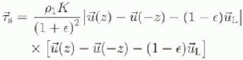
Near the air-sea interface the surface shear stress can be represented in both fluids by an aerodynamic bulk relationship which takes account of the wavefield (Bye, 1995). in the air, we have rs

and in the water,

where z = 0 is the mean interfacial level,  is the fluid velocity,
 is a non-wave-induced velocity, which will be called the reference velocity since it is common to both fluids,
 is the spectrally averaged phase velocity of the wave spectrum, and
 is The spectrally integrated surface Stokes velocity, where
 is a drag coefficient, pi
and p2
are respectively the densities of air and water, and
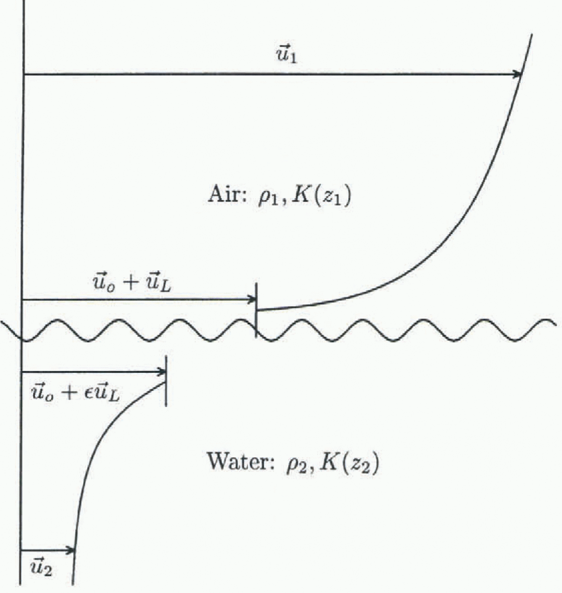
 is the interfacial shear stress (see Fig. 1). Equations (1a) and (1b) are assumed to apply within a wave boundary layer which extends upwards and downwards from the interface.
Schematic picture of the inertial coupling concept.  is the surface wind,
 is the reference velocity,
 is the phase velocity,
 is the surface current, pi is the air density, p2 is the water density,
 and K(zi) (i = 1,2) are the drag coefficients in air and water, respectively.
On equating (1a) and (1b) we obtain
and also the wave relation

The application of diese relations at the edge of the wave boundary layer ( ) at which
 is the surface wind, and
 is the surface current is considered in the situation in which the time mean reference velocity is

which is appropriate for the Earth reference frame. Equation (4) is assumed to be valid for a short-period averaging of the wind, and a long-period averaging of the current, for which Equation (3) (applied at the edge of the wave boundary layer) reduces to the expression

which predicts the surface Stokes drift ( ) in terms of
 and
 in a similar manner, the surface shear stress in the Earth reference frame
 is given by the relation,
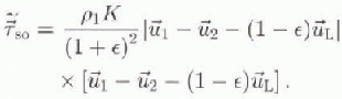
 , with
 given by Equation (5), is used to drive the oceanic circulation.
The solution predicts the current field ( )- From this prognosis, two physically important additional velocity fields can be determined diagnostically.
First, the surface velocity ( ) which consists of the sum of the fiuctuation in reference velocity (
 ) and the surface Stokes drift
 is obtained, which on using Equations (3) and (5) can be expressed as follows:

which is the sum of three terms: the surface Stokes drift, a fluctuation velocity due to the current, and a fiuctuation velocity due to the wind.  is applicable below the rotational turbulent interfacial layer which connects the two fluids (Bye, 1988a).
Secondly, we can determine diagnostically the surface drift velocity ( ) which is the vector which connects the two fluids through the turbulent interfacial layer. Us occurs at
 at which the velocities in the two tluids are equal, and on applying Equation (3) we obtain (Reference KrausKraus, 1977)

which on using Equations (3) and (5) can also be expressed in the form

Equation (3) indicates, since  , that the turbulent inter-facial layer approximately doubles the contribution to the total velocity due to the irrotational wavefield. The contributions due to the wind and current, however, are unchanged.
 is the velocity which would be expected to guide surface films. It is also possible that drift cards would travel at this velocity unless wave breaking causes the cards to temporarily lose contact with the water surface.
The three velocity fields ( and (
 ) are used to disperse simulated groups of particles.
The particular quasi-geostrophic solution that is used to disperse the particles is taken from the numerical study of Bye and Wolff (in press), in which the simulation was run for 2.4 X 10⁶ time-steps of 2 hours (approximately 5000 years), with a steady zonal wind and a current averaging period of 300 days. The domain consisted of an annulus of length 4000 km and width 1500 km in which a cyclic topography based on the Macquaric Ridge Complex was implemented with a mesh interval of 20 km (Wolff and others, 1991). A drag coefficient K = 4.8 X 10 −3 was used in Equation (6) with  and
 and the zonal wind field
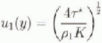
where

in which  and Y is the width of the channel. Full details of the solution are given in Bye and Wolff (in press). figure 2a, which shows the instantaneous solution in the upper layer at the end of the integration, indicates the level of eddy activity, and figure 2b shows the corresponding Stokes surface drift streamfield, obtained diagnostically from Equation (5).
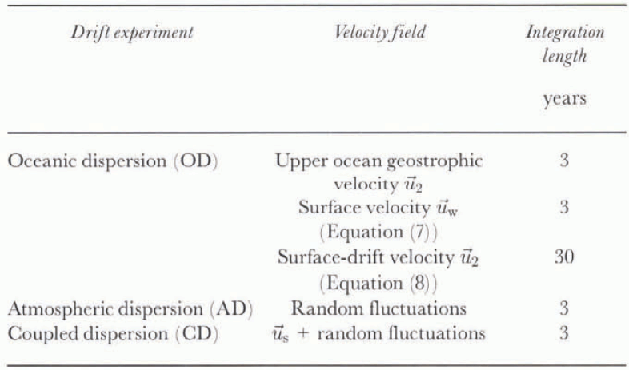
A group of 200 particles was released over an area of approximately 1° longitude by 2° latitude (90 X 190 km2) close to the centre of the model area. The particles were then advected by one of the velocity fields in Table 1 for the period indicated (3—30 years). The advecrion was computed with a very efficient fourth-order Runge Kutta scheme to account correctly for the curvature of the flow fields. Every twelfth
Stream functions of the Macquarie Ridge Complex experiment MCQS300 from Bye and Wolff (in press). (a) In-stantaneous stream function at the end of the integration in the upper layer (contour interval (CI) = 104m2S−1); (b) Stokes-drift stream function (CI =5 X 10³m2s−1).

Model experiments
timc-step(= 1day), the positions of all particles were recorded (starting 1 day after the release), and at the end of the integration, the standard deviations of the particle distributions at time (t) were obtained from the following formulae:
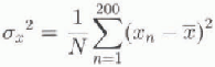
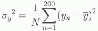

where ( ) are the co-ordinates of the centroid of the distri-bution. Trajectory plots were also obtained for a sample of 20 particles out of the 200 released.
The dispersion by wind fluctuations was investigated using a random model in which the fluctuation in wind at each gridpoint was created by a random number generator giving values between ±U, where U is a velocity scale. The standard deviation of the fluctuations is  .
4. Theoretical Background
The release of particles paints a Lagrangian portrait of the flow field, from which its turbulent properties can be deduced (Reference RodeanRodean, 1996). in this study, through the surface stress relation, we are able to examine the change in the two-dimensional turbulent field as a function of depth throughout the wave boundary layer in both fluids. The three velocity fields ( ) reveal this evolution of turbulent properties throughout the oceanic boundary layer. Any objects of finite draught respond to a depth average between these fields and also with respect to the corresponding velocity fields in the atmospheric boundary layer, the effect of which is usually called windage. in view of the simple representation of the atmospheric velocity used in this model in which “we have in reality supposed that we can divide the phenomenon into two parts, one (random) in which the discontinuity of the events taking place is essential while in the other (deterministic) it is trivial and can be ignored” (Chandrasekhar, 1943), windage is omitted in this study.
At each level, the interpretation of the results is based on the definition of the diffusion coefficient (Reference TaylorTaylor 1921),

where K1 and K2 are respectively the longitudinal and transverse coefficients. For a power law relation,

we obtain

where

Two important special cases of Equation (16) are:
-
(i) Brownian motion (mi = 1) for which bi = qi, = 0, and Ki = constant,
 which is the condition for an unbounded random walk.
-
(ii) Inertial (mi= 3) for which bi = 2, qi = 2/3, and
which applies for an inertial subrange in which dissipation is negligible.
 which is the condition for an unbounded random walk.
 which applies for an inertial subrange in which dissipation is negligible.
A comparison between the numerical experiments and a power law representation is not straightforward, due to (i) an initial adjustment period after the particles were released, and (ii) the boundary effects of the channel walls which become significant after long transit times.
Oceanic dispersion. Trajectories of the centroid of the particle distributions over a period of 3 years for the velocity fields  and
 .

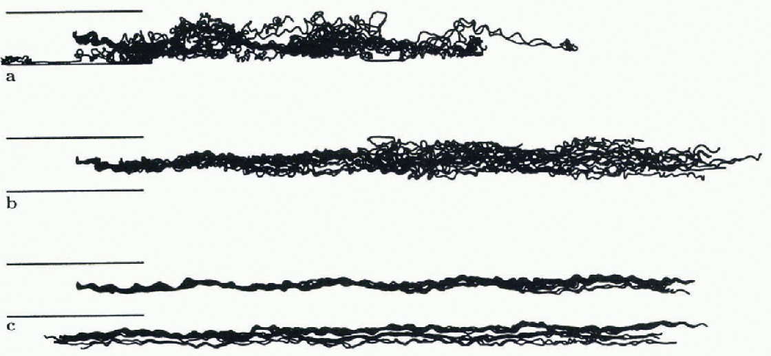
Particle clouds at the end of the dispersion experimentsfor the velocityfields (a)  , (b)
 and (c)
 . The particles have been trackedfor 3 years, and in (c) the tracks after 18 months have been continued one channel width below the first 18 months (to allow the same scale as in (a) and (b)). The two parallel lines to the left indicate the channel dimensions. See figure 5for the actual tracks of a sub-sample of particles.

In the channel, the longitudinal and transverse diffusion almost correspond with zonal and meridional diffusion, respectively (see Fig. 3), and in the discussion of the results we assume that  and
 (with 1 and 2 denoting the principal axes of the diffusion ellipsoid).
5. Results of the Dispersion Experiments
The three series of dispersion experiments (table 1) will be called (i) oceanic dispersion (OD) in which the fluctuations in the surface wind are zero, (ii) atmospheric dispersion (AD) in which only dispersion due to the wind fluctuations is considered, and (iii) coupled dispersion (CD) in which both diffusive processes are included. The three series will be considered in turn.
5.1. Oceanic dispersion (OD)
Figure 3 shows the progression of the centroids of the groups of particles released into the three velocity fields. It is apparent that the zonal propagation of the centroid for  is about twice that of
 (see Equations (7) and (9)), and that of
 is about 60% of
 , but until about 8000 km the three trajectories are fairly well correlated. Subsequently, the centroid of
 tends to a stationary limit with the onset of a well-mixed state. The trajectory of the centroid for
 , however, indicates that the particle group remains coherent throughout the experiment, i.e. for about eight revolutions of the model Antarctic Channel.
The corresponding particle clouds are shown in Figure 4. There is a strong anisotropy in the distributions. Figure 5 shows the tracks of a sample of 20 particles out of the 200 released; there is an obvious transition from the “spaghetti diagram” of the  field through to a “braided pattern” for the
 field. The particles in the
 dispersion experiment are also clearly affected by the southern boundary.
The statistics of the dispersion are shown in figures 6 and 7. in all the experiments there is an extended initial period of adjustment of about 4 months (107 S), after which the simulated data are fitted approximately by power law
Trajectories of a sample of 20 particles releasedinto the velocity fields (a)  , (b)
 and (c)
 . The particles have been trackedfor 3years, and in (c) the tracks after 18 months have been continued one channel width below the first 18 months (to allow the same scale as in (a) and (b)). The two parallel lines to the left indicate the channel dimensions.
The variance  of the longitudinal dispersion for oceanic dispersion in the velocity fields
 and
 . The variance (ordinate) is given in units of m2, and the time (abscissa) in units of s.

The variance  of the transverse dispersion for oceanic dispersion in the velocity fields,
 and
 . The variance (ordinate) is given in units of m2, and the time (abscissa) in units of s.

representations. For longitudinal dispersion the exponent (m
1) in Equation (16) is about 1.5 for the  and
 fields, whereas it has increased to about 2.5 for the
 field. For the transverse dispersion, on the other hand, m2
is very small in all experiments, in part due to boundary effects. The results, however, give the strong impression that in the absence of lateral boundaries the dispersion would still be strongly anisotropic
5.2. Atmospheric dispersion (AD)
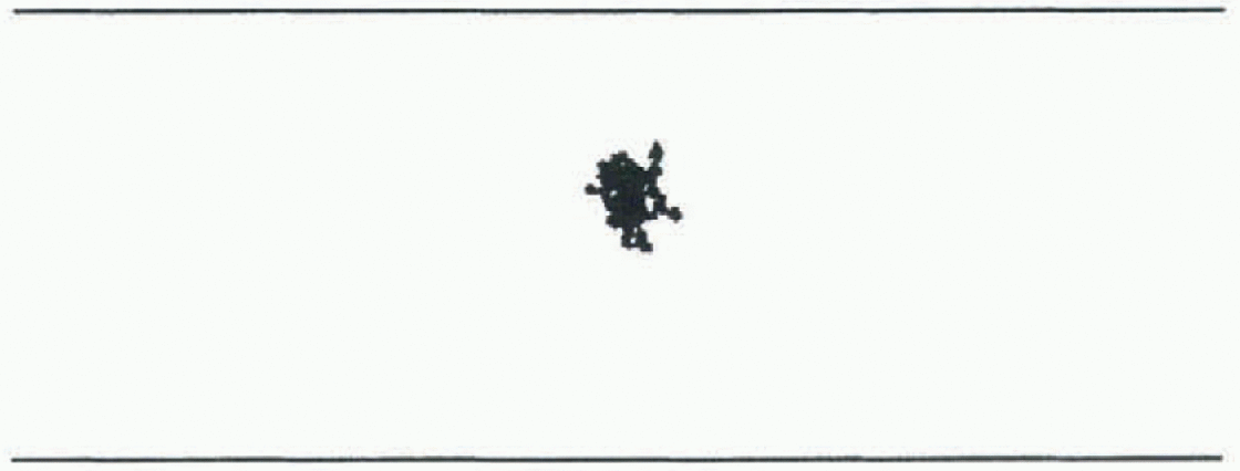
The dispersion due to wind fluctuations only is almost isotropic (Fig. 8), and for U = 5ms −1 it is confined centrally with in the channel. The zonal and meridional statistics are similar (Fig. 9), and the exponents tend to the random walk value, mi~1.
5.3. Coupled dispersion (CD)
The structure of simulations including both diffusive processes was found to be very similar to that with OD only. The only difference was that the levels of variance were somewhat elevated. Figure 10 is an extended run (for 30 years) with the นS field which shows the total variance ( ) with and without AD.
There are three notable features: (i) the power law slope is reasonably stable over the longer interval; (ii) the total variance ( ) is systematically greater for the CD solution compared with the OD solution; and (iii) the total variance (
 ) is almost identical to the longitudinal variance (
 ) (Fig. 6) for the OD solution.
Trajectories of a sample of 20 particles dispersed by random wind fluctuations with a velocity scale of U = 5ms−1.
6. Discussion
The following conclusions may be drawn from these experiments.
-
(a) Since the average eastward progression of objects in the Circumpolar Channel guided by the surface current (
) and by the surface velocity () is similar (Fig. 3), it is predicted that objects with a range of draughts would travel at about the same average speed (excluding cflccts of windage) in agreement with field observations (Lutjeharros and others, 1988; Large and Van Loon, 1989). The “spaghetti diagram” (fig. 5a) is typical of observations of satellite-tracked buoy trajectories. Figure 3 shows that surface drift can remain as a coherent pulse, possibly for a few global rotations, as is suggested by long-term drift-card experiments (Bye, 1988b), even though the cards may have been tumbled by wave action. -
(b) The dispersion process is strongly anisotropic (see figs 6 and 7). in these simulations, this behaviour clearly is not attributable to the shear effect, but arises from the aniso-tropy of the velocity field (fig. 2a). The effects of this anisotropy characterise the thermohaline structure of the Southern Ocean.
-
(c) The AD experiment suggests that OD dominates in the Southern Ocean. This conclusion, however, would need to be tested using a more realistic atmospheric synoptic forcing.
-
(d) The most interesting conclusion is that the inertial character of the turbulence which causes the dispersion increases as the sea surface is approached. The simulated power law behaviour for the surface-drift
) field (Fig. 10) is in remarkable agreement with observed surface-drift dispersion (Reference OkuboOkubo, 1971), in both energy and slope. There is no a priori reason to anticipate that the inertial power law slope of 3 should be obtained. in reality, the coupled system at the sea surface is probably sub-iner-tial, and even less inertial at depth.
 ) and by the surface velocity (
 ) is similar (
 ) field (
The variance  and
 for atmospheric dispersion with a velocity scale, U = 5 m s−1, The variance (ordinate) is given in units of in, and the time (abscissa) in units of s.
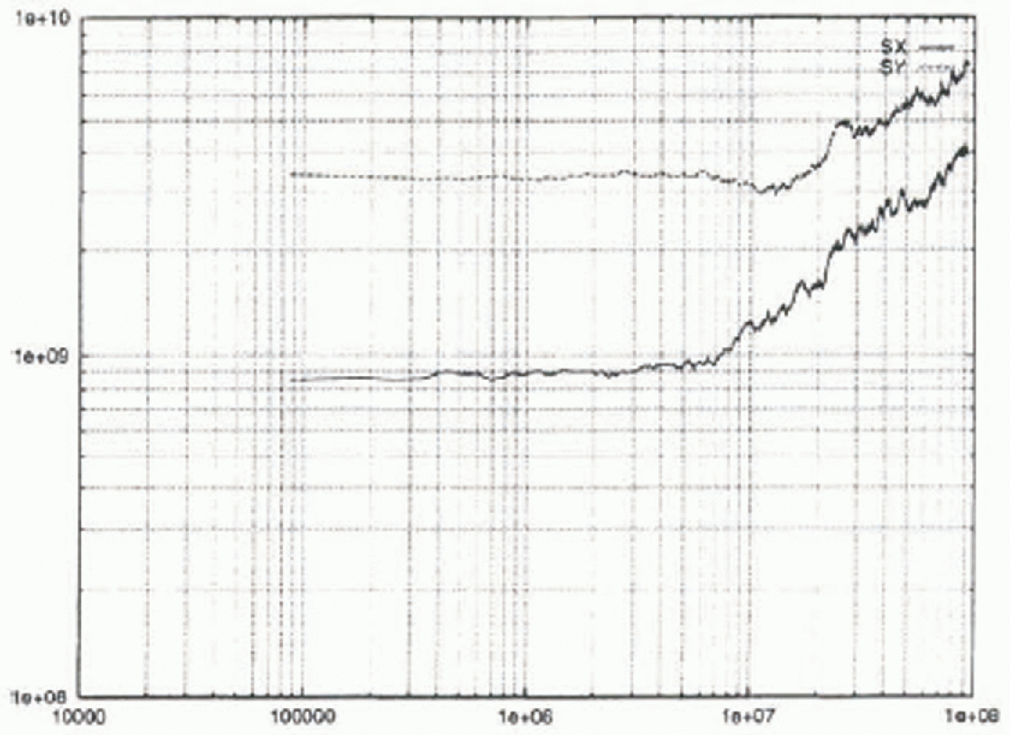
The total variance  for oceanic dispersion over an extended period (30 years), andfor coupled dispersion with
 . Indicated is the power law relation for observed diffusion from Okubo
 , where
 with A = 1.08 X 10⁻⁶. The variance (ordinate) is given in units of m2, and the time (abscissa) in units of s.

Another way of looking at the difference in the dispersion between the levels is that the expressions for  and
 consist of a steering velocity and a turbulent fluctuation. The steering velocity for
 is
 (Equation (9)), and for
 it is CUL (Equation (7)); similarly it is
 for
 , at which level the fluctuation due to the wind is absent, and that due to the current is just
 . The steering velocity increases towards the sea surface, especially between
 and
 , and this has the effect of increasing the exponent (
 ) in the dispersion diagram.



