

Introduction
Over the past few decades, India’s billion-plus population has experienced significant transitions in its key socioeconomic and demographic indicators. The most recent census of 2011 revealed that the national population growth rate had fallen well below 2% per annum – the first time since the 1980s (RGI, 2011a,b). This deceleration in the population growth rate, however, cannot by itself explain the magnitude and extent of the fertility transition underway across India. The reduction in fertility rates has been quite striking, with the Total Fertility Rate (TFR) dropping from 5.8 during the 1950s to 2.7 in the latter half of the 2000s. Estimates from the recent National Family Health Survey (NFHS-4) conducted in 2015–16 reported that, with the exception of twelve states located primarily in the country’s north–central and north-eastern regions, all other states had achieved replacement level fertility, further attenuating the aggregate TFR to 2.2 (IIPS & Macro International, 2017). However, with the country as a whole yet to arrive at this replacement level fertility (TFR<2.1), the existing obvious and marked geographic variations in fertility have been well documented (e.g. Murthi et al., Reference Murthi, Guio and Dreze1995; James, Reference James1999; Dreze & Murthi, Reference Dreze and Murthi2001; Sekher et al., Reference Sekher, Raju and Sivakumar2001; Bocquet-Appel et al., Reference Bocquet-Appel, Rajan, Bacro and Lajaunie2002; Guilmoto & Rajan, Reference Guilmoto and Rajan2002, Reference Guilmoto and Rajan2013; Rajan, Reference Rajan2005; Moore et al., Reference Moore, Singh, Ram and Audam2009; Kulkarni, Reference Kulkarni2011; Das & Mohanty, Reference Das and Mohanty2012; Dharmalingam et al., Reference Dharmalingam, Rajan and Morgan2014; Uttamacharya & Arokiasamy, 2014; Ghosh, Reference Ghosh2018).
While many studies, primarily based on the normative models of fertility differentials, have assessed this transition and its trajectories, their findings have been inconsistent and at times contradictory about the nature and magnitude of the factors that have been conducive to propagating it, and on their underlying regional differentials. For example, better health care services and improved educational facilities for women were considered to be the driving factors in Kerala, while the execution of various family planning programmes, media exposure and social movements by backward classes were upheld as being most relevant in Tamil Nadu for causing substantial fertility decline (Zachariah, Reference Zachariah1984; Bhat & Rajan, Reference Bhat and Rajan1990; Kulkarni et al., Reference Kulkarni, Krishnamoorthy and Audinarayan1995; Bhat, Reference Bhat1996; Zachariah & Rajan, Reference Zachariah and Rajan1997; Guilmoto & Rajan, Reference Guilmoto and Rajan2001, Reference Guilmoto and Rajan2005; Nair, Reference Nair2010; Kulkarni, Reference Kulkarni2011; Guilmoto, Reference Guilmoto2013). Contrastingly, analysing NFHS data, Vithayathil (Reference Vithayathil2013) argued that substantial female sterilization and the postponement of childbearing immediately after marriage had played key roles in the emergence of lower fertility in these two states. By and large, most traditional socioeconomic theories have postulated that a gradual adaptation to changing socioeconomic circumstances will cause fertility decline. Of late, however, much literature has made it evident that this may not be the case everywhere on the grounds that the pace and intensity of the behavioural adaptation to changing socioeconomic circumstances would differ markedly, based on the individual population’s characteristics and their own socio-cultural contexts (Bongaarts & Watkins, Reference Bongaarts and Watkins1996; Martine, Reference Martine1996; Kohler, Reference Kohler1997). For example, researchers have noticed sharp fertility declines in Andhra Pradesh, Gujarat and Bangladesh despite the female education level being very low in these regions (Visaria et al., Reference Visaria, Visaria and Jain1995; James, Reference James1999; Kabir et al., Reference Kabir, Barbhuiya and Islam2001; Dev et al., Reference Dev, James and Sen2002). Similarly, Dreze and Murthi (Reference Dreze and Murthi2001) found a very tenuous causality between relevant development and modernization indicators (i.e. poverty, male literacy and urbanization) and fertility rates across India’s districts and argued that fertility decline was not a mere ramification of economic development, but rather the betterment in certain conditions, which acted as a catalyst to alter couples’ fertility goals and help them comprehend which goals were essential. As a corollary, this failure in substantiating that a betterment in socioeconomic circumstances would always induce fertility decline, or could be used to chart fertility transitions, stimulated research on the new role of spatial externalities and innovation diffusion in fertility reduction (Carlsson, Reference Carlsson1966; Guilmoto, Reference Guilmoto2000; Arokiasamy, Reference Arokiasamy2009; Mohanty & Ram, Reference Mohanty and Ram2011). Recent evidence bears out that the substantial use of contraception by illiterate females in Andhra Pradesh and the resultant sharp decline in fertility rates has actually been facilitated by relevant information diffusion through health workers, via contact with other educated women and from exposure to media (Bramhanandam & Arokiasamy, Reference Brahmanandam and Arokiasamy2016). Sekher et al. (Reference Sekher, Raju and Sivakumar2001) also highlighted that a significant geographic inequality in fertility decline existed among the districts of Karnataka, with its southern and coastal districts recording a much faster fertility decline than its relatively more backward northern districts. This geographic variation in the pace of fertility decline also exhibits a conspicuous North–South divide across India, as surmised by other studies, with the sluggish rates prevalent in the northern states being reflective of them having a deeply rooted patriarchy, an agro-based economy and much lower female education levels (Guilmoto, Reference Guilmoto2000, Reference Guilmoto2013; Guilmoto & Rajan, Reference Guilmoto and Rajan2001).
Only a few studies in India have examined the low-fertility regimes arising from ideational and behavioural transformations in populations central to Second Demographic Transition (SDT) theory (see, Vithayathil, Reference Vithayathil2013; Dharmalingam et al., Reference Dharmalingam, Rajan and Morgan2014; Pradhan & Sekher, Reference Pradhan and Sekher2014; Ghosh, Reference Ghosh2017). These have broadly found that couples’ individual self-actualization, them having higher aspirations for their children and constraints and considerations in childbearing and childrearing have largely encouraged parents to accept single-child/small-size family norms. Yet, how well the existing fertility models can discern and decipher such low-fertility dynamics remains a matter of debate (Dharmalingam et al., Reference Dharmalingam, Rajan and Morgan2014). Aside from this, the results gleaned from quantitative research using secondary data have not always tallied with those from detailed primary surveys, in respect of the roles that particular indicators (e.g. income/economic development, programme implementation, education and media exposure) have played in influencing fertility behaviour (for a review, see Kulkarni, Reference Kulkarni2011).
Given the above context, it is argued that possibly the aforementioned inconsistencies in the findings gleaned from fertility studies in India may have arisen since the respective impacts of the driving forces on the fertility variations might have significantly differed geographically due to marked differences in their local contexts and underlying characteristics. Furthermore, the processes of fertility transitions are also crucially context-specific and vary across locations (Wang & Chi, Reference Wang and Chi2017). Prevalent fertility decline theories have long noted that fertility behaviour differs depending on how people are influenced by socioeconomic structures, socio-cultural interactions, externalities and programme/policy implementation strategies (Easterlin, Reference Easterlin1969; Cleland & Wilson, Reference Cleland and Wilson1987; Chamratrithirong et al., Reference Chamratrithirong, Hirschman and Guest1992; Montgomery & Casterline, Reference Montgomery and Casterline1993, Reference Montgomery and Casterline1996; Hirschman, Reference Hirschman1994; Bongaarts & Watkins, Reference Bongaarts and Watkins1996; Axinn & Yabiku, Reference Axinn and Yabiku2001; Amin et al., Reference Amin, Basu and Stephenson2002; Guilmoto & Rajan, Reference Guilmoto and Rajan2005; Paul & Kulkarni, Reference Paul and Kulkarni2006; Alagarajan & Kulkarni, Reference Alagarajan and Kulkarni2008; Kulkarni, Reference Kulkarni2011; Haque & Patel, Reference Haque and Patel2016; Ghosh, Reference Ghosh2017). Thus, spatially varying levels of socioeconomic development, demographic behavioural changes and differences in welfare and population policy implementation could also foster marked fertility variations across places and a single, one-size-fits-all model may not easily encapsulate such intricacies of the spatial dimensions of fertility differentials and their underlying correlates, and indeed how their inter-linkages might be shaped by the local geography. From a policy viewpoint, such inter-district differentials in fertility have crucial implications for local-level decentralized planning towards providing family planning, health care, education and other welfare services. Spatial variations in fertility rates also remain a major concern while administering national/sub-national-level population projections (Wilson, Reference Wilson2015). Furthermore, a nuanced, contextual comprehension of not only place-specific fertility patterns but also the correlates responsible for such fertility transition differentials across India is essential as it is expected to provide a deeper understanding of the extent to which regional fertility differentials might persist or converge in the near future, which may thus be advantageous for local-level planning.
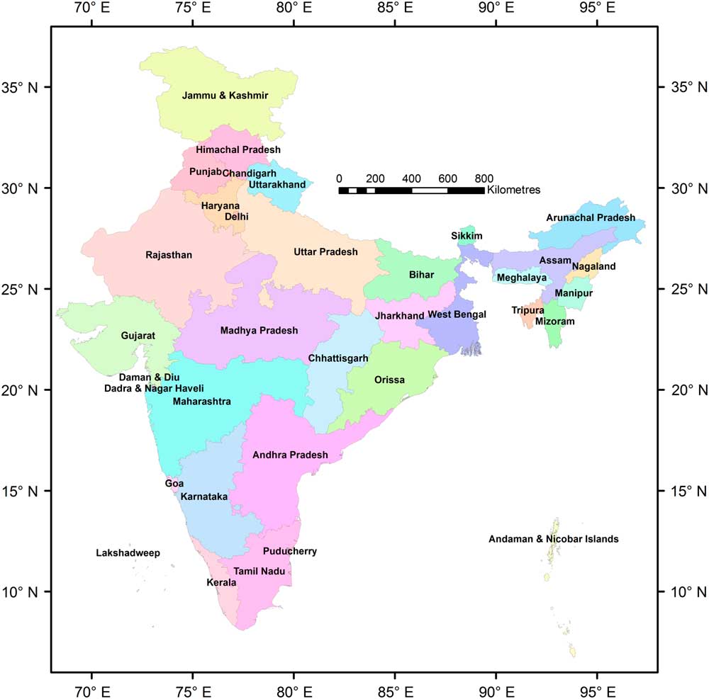
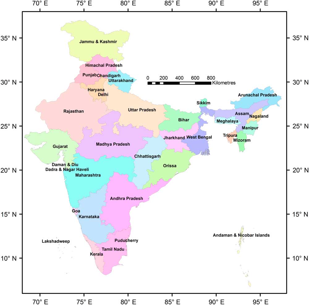
While considerable literature exists on India’s fertility differentials and its correlates, there is still a lack of conceptually and methodologically informed research on the spatial dimensions of fertility behaviour. Towards this end, this paper explicitly contributes by introducing geography into the debate, using the latest district-level census data for the whole country (see Figure 1; maps with the individual districts labelled for each state separately are also available from the authors on request). Initially, an assessment of the influence exerted by spatial autocorrelation upon fertility outcomes was modelled using two Spatial Auto Regressive models [SAR (lag/error)]. Then, to further comprehend the discerned spatially varying relationships, the Geographically Weighted Regression (GWR) technique (Fotheringham et al., Reference Fotheringham, Brunsdon and Charlton2002) was utilized. The outcomes were expected to reveal that ‘geography mattered’ in causing the marked fertility differentials across India, with the individual district-level demographic, socioeconomic and cultural characteristics precipitating different fertility outcomes, depending on the respective district location. The performance and prediction accuracy of the SAR and GWR models were also examined and compared with the results derived from the conventional non-spatial Ordinary Least Square (OLS) model, for a deeper understanding of how linkages between the districts’ fertility rates and their commonly perceived driving forces varied across locations. The significance of inculcating spatial dependence and heterogeneity in fertility research for deciphering local patterns and drivers was thus highlighted.
States and Union Territories of India
Spatial dependence/heterogeneity and fertility outcomes: some theoretical considerations
Many studies have attested that spatial dependence crucially governs social issues and behaviour, including demographic, socioeconomic and political changes (Morenoff & Sampson, Reference Morenoff and Sampson1997; Morenoff et al., Reference Morenoff, Sampson and Raudenbush2001; Noonan, Reference Noonan2005; Işik & Pinarcioğlu, Reference Işik and Pinarcioğlu2006; Swaroop & Morenoff, Reference Swaroop and Morenoff2006; Crowder & South, Reference Crowder and South2008; Millward, Reference Millward2008; Baumont, Reference Baumont2009; Taiwo & Ahmed, Reference Taiwo and Ahmed2015; Evans & Gray, Reference Evans and Gray2017; Saha & Paul, Reference Saha and Paul2017; Wang & Chi, Reference Wang and Chi2017). Thus in assessing geographical attributes and cross-sectional data, location plays a key role in precipitating spatial effects – i.e. spatial heterogeneity and autocorrelation (Yu et al., Reference Yu, Wei and Wu2007), with the spatial autocorrelation being a ‘similar juxtaposition or meeting of the locational similarity with the value similarity’ (Anselin, Reference Anselin2001).
Primarily, traditional fertility research in India, building upon the classical demographic transition theory (Easterlin & Crimmins, Reference Easterlin and Crimmins1985; Kirk, Reference Kirk1996), had accentuated the influence of socioeconomic, development and demographic factors in fertility decision-making, since these were closely linked to policy debates on the need for government interventions in carrying through ongoing fertility transitions. These, however, neglected the spatial effect on fertility behaviour (e.g. rural–urban fertility differentials: Robinson, Reference Robinson1961; Sharma & Pandey, Reference Sharma and Pandey2000; Moore et al., Reference Moore, Singh, Ram and Audam2009; Kulkarni, Reference Kulkarni2011). More recently, fertility decline has become perceived as being far from a universal theory, to the extent that ‘distinct historical and geographical contexts reveal more diversity than those which a simple theory of fertility transition would predict’ (Hirschman, Reference Hirschman1994, cited in Wang & Chi, Reference Wang and Chi2017), and alternative research outlooks have been adopted. As surmised in Wang and Chi (Reference Wang and Chi2017), such countervailing arguments have stressed how knowledge diffusion and social mores and interactions have influenced and continue to mould fertility behaviour (Cleland & Wilson, Reference Cleland and Wilson1987; Montgomery & Casterline, Reference Montgomery and Casterline1993, Reference Montgomery and Casterline1996; Hirschman, Reference Hirschman1994; Bongaarts & Watkins, Reference Bongaarts and Watkins1996; Axinn & Yabiku, Reference Axinn and Yabiku2001; Arokiasamy, Reference Arokiasamy2009). This diffusion mechanism is likely to advance spatially over time, quite independently and rapidly, compared with the socioeconomic improvement induced decline in fertility rates (Retherford, Reference Retherford1985; Montgomery & Casterline, Reference Montgomery and Casterline1996; Lesthaeghe & Vanderhoeft, Reference Lesthaeghe and Vanderhoeft2001). Reductions in fertility rates in developing nations have also been attributed to different types of diffusion mechanisms, like social interactions and contact between geographically proximate neighbourhoods (Casterline, Reference Casterline2001; Amin et al., Reference Amin, Basu and Stephenson2002; Bongaarts, Reference Bongaarts2002). Therefore populations at geographically proximate locations are more likely to exhibit similar fertility outcomes, since while taking life-course and fertility-related decisions (e.g. education, age at marriage, childbearing, family size, family planning), couples would not consider simply their own circumstances but also learn from, and simulate the fertility behaviour of, their neighbours (Wang & Chi, Reference Wang and Chi2017). Hence, the spatial patterning of fertility decline would not simply reflect the underlying socioeconomic attributes and structural changes, but also be indicative of demographic behavioural changes through geographical diffusion of information, ideas, technological innovations, prevalent norms and institutional practices (Li, Reference Li1973; Basu & Amin, Reference Basu and Amin2000; Casterline, Reference Casterline2001; Amin et al., Reference Amin, Basu and Stephenson2002; Arokiasamy, Reference Arokiasamy2009; Cai, Reference Cai2010) and spatial autocorrelation in fertility rates might also result in such settings (e.g. a similar level of economic development, homogeneity in population in terms of religion, caste, ethnicity, language or class identity and government specific modus operandi towards implementation of various welfare schemes and family planning programmes). These eventually would develop a spatial clustering of fertility patterns by grouping together neighbourhoods having the same conditions in terms of neighbourhood externalities and spatial diffusions. Furthermore, as there have been marked and well-documented regional differentials in fertility transition across India, due to an uneven distribution of people from various castes/classes/religions across districts (Alagarajan & Kulkarni, Reference Alagarajan and Kulkarni2008), the varying fertility outcomes might well be the result of similar spatial spill-over effects (the fertility character of one neighbourhood influencing to some degree the same attribute of its adjacent neighbourhoods, especially if there exist common demographic or socioeconomic traits between the two) and spatial diffusion.
Spatial heterogeneity, however, implies a non-stationary mechanism over geographic locations, wherein areas with similar socioeconomic/demographic attributes may exhibit varying fertility outcomes based on their different geographic locations (Fotheringham et al., Reference Fotheringham, Brunsdon and Charlton2002). India’s great socio-cultural and economic diversity, along with the regionally varying levels of urbanization, migration, rural–urban interaction, social and ideational transformation through diffusion channels and differing rates of behavioural adjustment to changing socioeconomic circumstances, including due to institutional reforms, creates a heterogeneous and segmented populace, with the northern and southern Indian states having consistently displayed two distinct demographic regimes having high and low fertility rates, respectively (Dyson & Moore, Reference Dyson and Moore1983). Thus, the district fertility rate and its socioeconomic–demographic linkages may not be stationary in nature and the history and geographical setting of an area may also affect its fertility outcome (Basu & Amin, Reference Basu and Amin2000; Amin et al., Reference Amin, Basu and Stephenson2002). Therefore it is paramount that the prevalent spatial effects (i.e. spatial autocorrelation and heterogeneity) be considered in such studies.
This paper is based on a number of spatial analyses methods that have examined the variations in fertility transitions from the viewpoint of examining how geography has influenced the spatial patterning of fertility behaviour. For instance, in an earlier attempt, Montgomery and Casterline (Reference Montgomery and Casterline1993) used a spatial econometric approach to assess the diffusion of fertility decline in Taiwan and commented on the crucial role of the diffusion process within and between the examined spatial units. Using a fixed-effect panel regression, Dreze and Murthi (Reference Dreze and Murthi2001) observed that geographic locations exerted a strong effect on fertility variations, despite controlling for other covariates, with fertility being higher in the northern regions and lower in the southern states of India. Apart from this, female education facilities and literacy, infant mortality and son preference emerged as crucial factors affecting fertility variations across India, over time, even when controlling for district effects. Analysing data for Bihar and Uttar Pradesh using multilevel regression, Das and Mohanty (Reference Das and Mohanty2012) found that controlling for all factors, 54% and 46% of the respective variance in the TFR was attributable to the district- and state-level differences. In a seminal work, Goldstein and Klusener (Reference Goldstein and Klüsener2014) analysed the geographic and structural factors of historical fertility decline in Prussia, using spatial econometric modelling. Considering religion, education, women employment status, income, urbanization, occupational hierarchy, infant mortality rates and adult sex ratio as covariates, they demonstrated that both socio-cultural and economic structural indicators emerged as significant predictors of fertility reduction. However, bereft of controlling for social interactions between proximate geographic regions, their estimates were unable to explain the geographic patterns of the noticed fertility decline, which resonated with the surmises made from the Princeton European Fertility Study (Knodel & Van de Walle, Reference Knodel and van de Walle1986).
Recently, a few studies have used the GWR local model to assess spatial heterogeneity in fertility outcomes. Işik and Pinarcioğlu (Reference Işik and Pinarcioğlu2006) examined Turkey’s fertility decline trajectories using GWR regression and found a spatially varying strong influence of the adult literacy rate, working women, GDP per capita, urbanization and migration rates on the fertility, across that country’s districts. Another by Evans and Gray (Reference Evans and Gray2017) in Australia, based on the GWR model, showed that around large urban centres, major fertility variations could be explained by the socioeconomic compositional differences of the locales, whereas in rural settings, deciphering these fertility differentials was quite difficult. Similarly, Wang and Chi (Reference Wang and Chi2017) surmised that the linkages between the county-level TFR and education for females, net migration, standard of living, place of residence, ethnicity/minority status, Sex Ratio at Birth (SRB) and fertility policy compliance ratio differed geographically, with respect to direction, magnitude and strength across China, indicating the strong spatial effect on fertility variations.
The foregoing theoretical underpinnings and research findings thus suggest that ignoring the spatial dependence/heterogeneity in such empirical research that deals with spatial data, could result in severe statistical problems (Can, Reference Can1992). Neglecting spatial autocorrelation while running a conventional OLS model would bias the standard errors downward, with the estimated coefficients being erroneous or deceptive (Anselin, Reference Anselin1988). To overcome this, both the SAR models (lag/error) were used to negate any spatial effect on the coefficients (Yu et al., Reference Yu, Wei and Wu2007). To address the spatial heterogeneity issue, carefully chosen interactions between the socioeconomic factors and location-specific dummy variables in a single model may be employed (e.g. Dreze & Murthi, Reference Dreze and Murthi2001), based on an intrinsic understanding of those particular interaction types. Techniques like the spatial expansion method and multilevel modelling, which have examined such local contexts, have generally utilized an a priori functional form that generated the nature of the spatial mechanism being modelled as either deterministic or discrete (Fotheringham et al., Reference Fotheringham, Brunsdon and Charlton2002; Das & Mohanty, Reference Das and Mohanty2012). This paper, contrastingly, has furthered the concept of spatial non-stationarity in fertility behaviour through GWR analysis (Fotheringham et al., Reference Fotheringham, Brunsdon and Charlton2002), by incorporating positional sites into the model rather than inculcating any a priori information on the fertility decline mechanism or its underlying processes. Thereby it accounted for the existent spatial heterogeneity in a more nuanced manner.
Formulated and examined hypotheses
A mixed theoretical approach was used for this research: adaptationist (adjustment to socioeconomic change, which is central to classical fertility theories) and diffusionist (diffusion of information through mass media or social interaction, i.e. norms/social acceptability of smaller family size; see Retherford, Reference Retherford1985; Harrell et al., Reference Harrell, Wang, Hua, Santos and Zhou2011; Goldstein & Klusener, Reference Goldstein and Klüsener2014). This was used since, out of the 621 studied districts across India, the TFR of 431 districts (69%) ranged from 2.1 to 5.8. Many districts were in different phases of fertility transition or were yet to break through the barrier and exhibited marked unequal socioeconomic development, coupled with extremely heterogeneous cultural, religious and linguistic composition. Consequently, the pace and intensity of the behavioural adjustment to changing socioeconomic circumstances also varied greatly among them. Therefore, while for most districts, the TFR variations could still be understood within the classical framework, in limited areas (e.g. Kolkata in eastern India) the lowest-low fertility clusters could also be reflective of a new fertility regime that hinted at the initiation of the Second Demographic Transition (Vithayathil, Reference Vithayathil2013; Ghosh, Reference Ghosh2017). Considering these facts, it could be reasonably expected that the pace of fertility decline and its spatial variations might be best explained by a joint venture of structural changes in socioeconomic circumstances and the diffusion of information/innovation abetting social change across India.
In contrast to previous such research, no prior assumptions of the model structure specifics were made (e.g. north–south divide or rural–urban gradient), nor were any universal relationships sought, with the focus being on deciphering the nature of spatial dependence and non-stationarity of fertility behaviour across the country. Numerous studies have highlighted the emergent patterns of low fertility in some parts of India (Dharmalingam et al., Reference Dharmalingam, Rajan and Morgan2014; Pradhan & Sekher, Reference Pradhan and Sekher2014), with some also examining the lowest-low fertility (TFR<1.3) levels in some districts (see Ghosh, Reference Ghosh2017). Although such in-depth investigations are beyond this paper’s remit, the factors underpinning distinctive fertility behaviour in low-fertility settings have been analysed using GWR local regression.
While the relationship between economic development/modernization (income/urbanization) and fertility decline, especially in India, has seldom been straightforward (Dreze & Murthi, Reference Dreze and Murthi2001), hinging on the micro-dynamics between pronatalist societal norms and antinatalist fertility laws (Greenhalgh & Winckler, Reference Greenhalgh and Winckler2005; Zhang, Reference Zhang2007; Peng, Reference Peng2010), recent research has revealed the adoption of single-child/small-family norms, with the acceptance that ‘fertility is a matter of choice’, in many locales, even rural ones (Kulkarni, Reference Kulkarni2011; Pradhan & Sekher, Reference Pradhan and Sekher2014; Ghosh, Reference Ghosh2017). The female education level has been historically considered most crucial in causing fertility decline (United Nations, 1973; Coale & Watkins, Reference Cole and Watkins1987; Dreze & Murthi, Reference Dreze and Murthi2001; Das & Mohanty, Reference Das and Mohanty2012), with better-educated women being more likely to join the workforce and transform their outlooks, aspirations and life-paths (Klasen & Launov, Reference Klasen and Launov2003; Jones, Reference Jones2007; Malhotra & Riley, Reference Malhotra and Riley2009; Aassve et al., Reference Aassve, Goisis and Sironi2012; Skirbekk & Samir, Reference Skirbekk and Samir2012), filling non-familial roles and gaining prestige (Ryder, Reference Ryder2010, cited in Ghosh, Reference Ghosh2017), thereby facing higher opportunity costs of childbearing (Becker, Reference Becker1960) or of staving off childbirth to meet career goals (Ghosh, Reference Ghosh2017). Indian Muslims have historically exhibited higher fertility rates than non-Muslims/Hindus due to religious factors or differential socioeconomic status (Alagarajan, Reference Alagarajan2003; Bhagat & Praharaj, Reference Bhagat and Praharaj2005; Alagarajan & Kulkarni, Reference Alagarajan and Kulkarni2008; Haque & Patel, Reference Haque and Patel2016; Pasupuleti et al., Reference Pasupuleti, Pathak and Jatrana2016; Ghosh, Reference Ghosh2018), while Scheduled Caste and Scheduled Tribe (SC/ST) groups have outranked other caste groups (for review, see Davis, Reference Davis1946; Nagdeve, Reference Nagdeve2012), with fertility attributes and adoption/diffusion of norms/behaviour being similar within such homogeneous entities (Attané & Courbage, Reference Attané and Courbage2000; Childs et al., Reference Childs, Goldstein, Jiao and Beall2005; Poston et al., Reference Poston, Chang and Dan2006). The difference in socioeconomic status among such caste-based groups can also influence their access to health care and nutrition, consequently resulting in differing fertility rates (Planning Commission, Reference Planning Commission2008, based on NFHS-3 data of 2005–06). Attitudes regarding contraceptive practices and better living standards (by accepting smaller family ideals) have been much influenced by mass media and greater degrees of social interaction (diffusion process) (Haque & Patel, Reference Haque and Patel2015), as evident in Andhra Pradesh, which attained low fertility in the 1990s despite having higher mortality and lower literacy rates than the national average (James, Reference James1999; Kulkarni, Reference Kulkarni2011; Brahmanandam & Arokiasamy, Reference Brahmanandam and Arokiasamy2016), notwithstanding the expected ‘threshold socioeconomic effects’ (Jain, Reference Jain1981), before this media influence could become operative. The above observations allowed the framing of some hypotheses, as follows:
H1: While economic development would usually result in fertility decline, this would not be the case always as in some locales affluent parents would prefer to have more children, being better able to bear the costs of childbearing/childrearing (possibly assuming children to be a source of economic security). Similarly, fertility behaviour would differ considerably from rural to urban areas, but rural areas would not always have higher fertility levels.
H2: Female education levels would be negative and significantly related to fertility rates but poor explanatory power was expected in some places where traditional family norms were still strongly prevalent.
H3: Different fertility patterns would be evident in districts which had higher concentrations of religious minorities (Muslims) or socially deprived groups (SC/ST).
H4: A significant negative relationship would exist between the exposure to mass media (proxy for diffusion of information) and fertility rates. However, areas in extreme poverty would not reflect the expected negative relationship between mass media exposure and fertility levels.
H5: The spatial clustering of low fertility levels would not be always adequately explained by its commonly regarded influencing factors like socioeconomic, demographic, cultural or policy attributes (i.e. probable relatively poorer model fits in areas where low fertility rates were clustered).
Methods
Data
While the Indian Census of 2011 provides extensive household-level data on demographic, literacy, socioeconomic and housing attributes, it does not give any direct estimates of the average number of children per woman, at the state/union territory (UT) level. Nor does the NFHS provide such estimations beyond the state/UT level. With this in mind, Guilmoto and Rajan (Reference Guilmoto and Rajan2002, Reference Guilmoto and Rajan2005, Reference Guilmoto and Rajan2013) gave estimates of the district-level TFR from census data, having argued that if the variations between states/UTs were justifiably ranged (e.g. from a TFR of 1.7 in Kerala in 2009 to 3.9 in Bihar), then the differentials across districts within a single state could also be significant since these were large administrative units (231 of India’s 640 districts have a population of more than 2 million people), especially within the most populous states like Uttar Pradesh or Madhya Pradesh (Guilmoto & Rajan, Reference Guilmoto and Rajan2013). A detailed depiction of fertility levels across all districts of the country would thus enable a better comprehension of the different rates and modes of fertility transition, in the context of separate geographical regions and for the country as a whole. For this study, the district-wise TFR values as estimated by Guilmoto and Rajan (Reference Guilmoto and Rajan2013) for 621 districts of India have been used to construct a comprehensive geo-coded database, along with the inclusion of other relevant parameters.
Dependent variable
To examine the spatial dynamics of the district-level fertility rate and its predictors, the TFR (2011) was taken as the dependent variable in the ensuing econometric estimations.
Independent variables
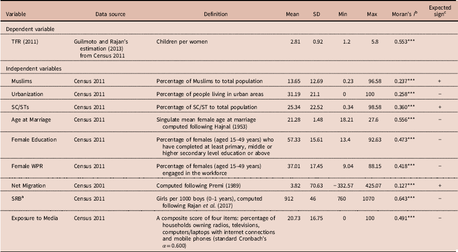
After reviewing similar ecological analyses of district-level fertility variations (Dreze & Murthi, Reference Dreze and Murthi2001; Das & Mohanty, Reference Das and Mohanty2012; Wang & Chi, Reference Wang and Chi2017) and in keeping with the formulated hypotheses, the analysis was restricted to examining nine commonly considered independent variables (Table 1), grouped as follows.
Descriptive summary of the studied variables at the district level in India (N=621)

a Since the analysis was based solely on census data and reliable estimations of the SRB were hardly available at the district level from the Sample Registration System (SRS) in India, the SRB was computed from the relevant census data on recent births, which may not be entirely reliable. This potential data limitation and measurement issue is acknowledged.
b Moran’s I is computed based on a 4.051544 degree Euclidian distance matrix.
c This denotes the expected relationship with the TFR in the global model.
Source: authors’ own calculations.
***p<0.001.
Sociocultural factors
Diverse cultural and regional factors influence India’s fertility patterns (Dyson & Moore, Reference Dyson and Moore1983; Basu, Reference Basu1992; Bhat, Reference Bhat1998; Maharatna, Reference Maharatna2000; Dreze & Murthi, Reference Dreze and Murthi2001). Muslims exhibit relatively higher fertility than other communities, but the degree to which this causality remains constant, when controlling for the socioeconomic disadvantages (i.e. poor social development and lower financial well-being) faced by them, is questionable (Alagarajan & Kulkarni, Reference Alagarajan and Kulkarni2008; Haque & Patel, Reference Haque and Patel2016). Similarly, SC/STs remain residentially most segregated (Vithayathil & Singh, Reference Vithayathil and Singh2012; Haque, Reference Haque2016; Haque et al., Reference Haque, Das and Patel2018) and socio-culturally different from the rest of the population. With distinct gender norms and kinship structure, including a higher rate of women workforce participation, they may contribute to fertility decline. South India has traditionally been a matriarchal society and women are accorded higher status, which may foster lower fertility rates (Dreze & Murthi, Reference Dreze and Murthi2001). Furthermore, fertility variations often overlap with sociocultural/political borders, as the diffusion of fertility norms, behaviour and technological innovations occurs faster within homogeneous populations who share a common cultural space (religious practices or language), as made evident by the Princeton European Fertility Studies (Coale & Watkins, Reference Cole and Watkins1986). Therefore, distinctive fertility patterns can be expected in areas where a particular community is dominant.
Economic development/modernization factors
The role of urbanization in fertility decline has also been much highlighted (Schulz, Reference Schultz1981, Reference Schultz1994; Bhagat, Reference Bhagat2011). Urbanization is taken as a vital indicator of regional/economic development, symbolizing the modernization central to the demographic transition theory (Dreze & Murthi, Reference Dreze and Murthi2001; Saha & Paul, Reference Saha and Paul2017). Urbanization causes fertility decline through two pathways: firstly, the role of children as a contributor to the household production becomes less prominent and, due to the rising cost of living in an urban setting, larger families find it very difficult to survive. Secondly, the urban area can be perceived as an epicentre for the rapid diffusion of information, sociocultural–normative–ideational changes and technological innovation, wherein individuals have a higher exposure to different media and through it are accorded many opportunities to interact with other social groups, which may foster demographic behavioural change and encourage fertility decline. For example, India’s leading metro cities (Kolkata, New Delhi, Mumbai and Bangalore) and their adjoining districts have emerged as early centres of fertility decline (Guilmoto & Rajan, Reference Guilmoto and Rajan2002). A negative urbanization–TFR relation is thus expected.
Social development/women empowerment factors
The importance accorded to Female Education in causing fertility decline has been discussed previously in the Hypothesis section. Together with this, the Female Work Participation Rate (Female WPR) considers the growing engagement of women in the workforce arising from modernization, economic liberalization and societal changes, enabling them to better realize their fertility goals. Being employed empowers and accords women direct access to the non-domestic environment and consequent control over monetary resources, ‘morphing’ them (Kishor, Reference Kishor1995; James, Reference James1999). This also reflects the modernization assumptions central to the demographic transition theory. Educated working women are more likely to follow a systematic life course with delayed marriage, late childbearing, higher birth spacing, including higher contraceptive use/or being sterilized, thereby encouraging fertility decline (Vithayathil, Reference Vithayathil2013). Both these variables were expected to flag a negative relationship with fertility rates in the global model.
Demographic factors
Age at Marriage has been cited as a strong determinant of fertility at both the aggregate as well as individual levels (Kulkarni, Reference Kulkarni2011), and was expected to have a negative relationship with the district-level fertility rate. Recent research has re-asserted that an early/lower age at marriage potentially contributes to higher fertility rates (Das & Mohanty, Reference Das and Mohanty2012). Net Migration was incorporated into the model to capture possible migration effects. A positive value of the net migration rate implied migration inflow, whereas a negative value indicated migration outflow, even though studies suggest that the association between fertility and spatial mobility is rather complex (Kulu, Reference Kulu2005). There are various types of spatial mobilities (e.g. urban to urban or rural to urban) and the migrants’ acclimatization pace and acceptance of a new environment, or of the prevalent norms, at their respective destinations varies markedly based on their individual characteristics and cultural aspects. Usually, migrants to urban areas adapt to the existing urban fertility norms within a short period of time and an overall positive causality between net migration and TFR was thus expected (Işik & Pinarcioğlu, Reference Işik and Pinarcioğlu2006; Wang & Chi, Reference Wang and Chi2017). A skewed Sex Ratio at Birth (SRB) has consistently been a serious concern in India (Saha & Paul, Reference Saha and Paul2017; Guilmoto et al., Reference Guilmoto, Saikia, Tamrakar and Bora2018) and one of the prime reasons for this has been strong son preference/gender discrimination. In India as a whole, both fertility attitude and behaviour are greatly influenced by a persistent son preference that is deeply rooted in the cultural traditions of Indian society and this adversely affects the reproductive behaviour of people, especially in their use of contraception and family planning methods, thereby hindering fertility decline (Das Gupta, Reference Das Gupta1987; Murthi et al., Reference Murthi, Guio and Dreze1995; Das Gupta & Bhat, Reference Das Gupta and Bhat1997; Mutharayappa et al., Reference Mutharayappa, Choe, Arnold and Roy1997; Kulkarni, Reference Kulkarni1999; Dreze & Murthi, Reference Dreze and Murthi2001; Arokiasamy, Reference Arokiasamy2002; Haque & Patel, Reference Haque and Patel2015). The SRB was included in the model to account for the son preference effect on fertility variations and a negative relationship was expected in the global model, i.e. a more balanced SRB would relate to a lower TFR.
Diffusion of information
The last covariate was Exposure to Media (a proxy measure of information diffusion). Previous research has shown that the diffusion of information and technological innovations through mass media or social interactions brings ideational and behavioural changes (central to the SDT theory) in populations (Vithayathil, Reference Vithayathil2013; Ghosh, Reference Ghosh2017). A higher exposure to mass media (through radio, television, newspapers, internet or mobile phones) and interactions with other individuals would alter demographic behaviour leading to the acceptance of family planning, limiting of family size or higher birth spacing and cause fertility decline (Das & Mohanty, Reference Das and Mohanty2012; Haque & Patel, Reference Haque and Patel2015; Brahmanandam & Arokiasamy, Reference Brahmanandam and Arokiasamy2016). Overall, greater Exposure to Media was thus expected to negatively influence fertility outcomes.
Analytical strategy
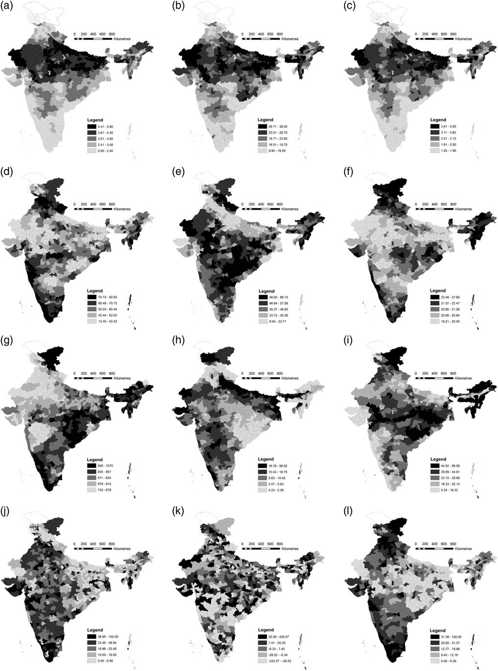
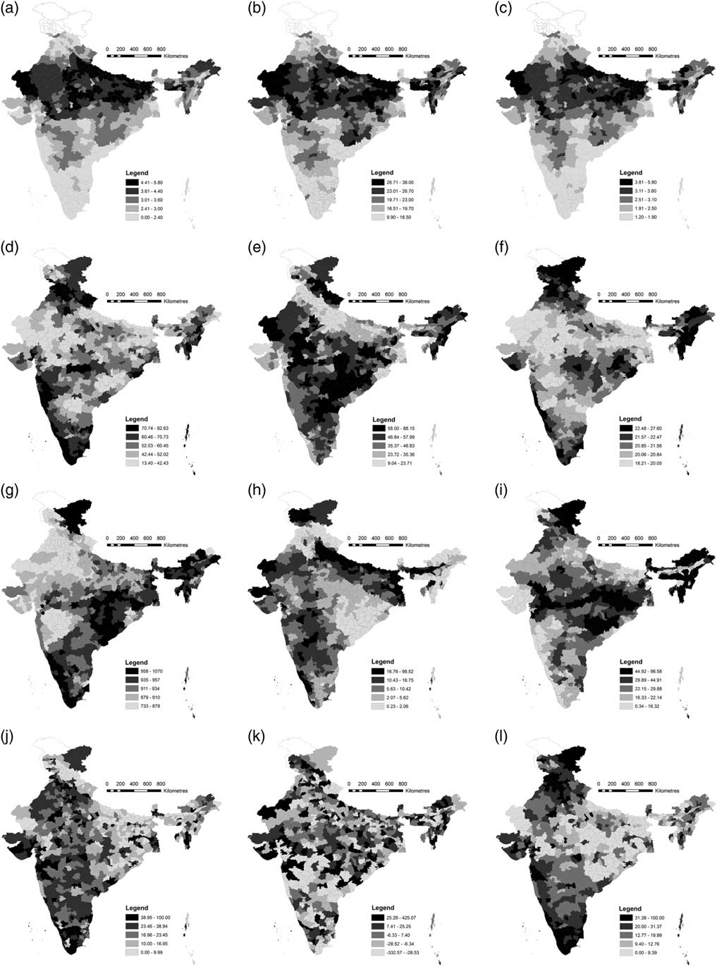
First, univariate descriptive statistics were estimated to understand the nature of variable distribution across the districts and all sample variables were mapped to discern their spatial distribution patterns (Fig. 2). Moran’s I statistics and the Local Indicator of Spatial Association (LISA) cluster maps were then prepared to assess the univariate global and local patterns of spatial dependence in these district-level fertility patterns (Anselin, Reference Anselin1996; Bivand & Piras, Reference Bivand and Piras2015).
Spatial distribution of the selected variables. (a) TFR (2001); (b) Crude Birth Rate (2011); (c) TFR (2011); (d) Female Education; (e) Female WPR; (f) Female Mean Age at Marriage; (g) Sex Ratio at Birth (SRB); (h) Muslims; (i) Percentage of SC/STs; (j) Urbanization; (k) Net Migration; (l) Exposure to Media. Values are presented in quintile scales. Source: same as Table 1.
Two types of spatial econometric regression analyses were run to detect spatial autocorrelation and heterogeneity in the fertility rates. First the global coefficients were estimated for the independent factors by using both the OLS and the SAR (lag/error) models. For spatial modelling, a spatial weight matrix, W, which considered the spatial structures of the districts, was generated considering the distance-based weight matrix, following Yu et al. (Reference Yu, Wei and Wu2007). Finally, the local coefficients were estimated using the GWR model. The performances of these three models were then examined and compared. Software packages GWR 4.0, ArcGIS 10.1 and GeoDa 1.8 were used for the various spatial and statistical analyses.
Model specification
The basic OLS model was specified as:
 $$Y_{{({\rm TFR}2011)i}} {\equals}\beta _{0} {\plus}\mathop \sum\nolimits_{i{\equals}1}^9 \left( {\beta _{i} X_{i} } \right){\plus}{{\varepsilon}}_{{i}} $$
where the dependent variable
 $Y_{{\left( {TFR2011} \right)i}} $
is the TFR of the i th district and
 $X_{i} $
denotes its vector for the select independent variables Muslims, Urbanization, SC/STs, Female Education, Female WPR, Age at Marriage, Net Migration, SRB and Exposure to Media;
 $\beta _{{0{\rm }}} $
and
 $\beta _{i} $
denote the intercept and regression coefficients, respectively, while
 ${\varepsilon}_{i} $
is an i.i.d. error term. The value of the mean Variance Inflation Factor (VIF) was 2.63.
Two Spatial Autoregressive (SAR) model techniques were used for infusing spatial autocorrelation into the models: the lag (or the substantive; Anselin & Rey, Reference Anselin and Rey1991) and the error (or nuisance) autoregressive specifications. The mathematical form of the autoregressive model was as follows:
 $$y{\equals}\rho Wy{\plus}\beta X{\plus}{\varepsilon}$$
where
 $\rho $
is the simultaneous autoregressive lag coefficient, Wy denotes the spatially lagged dependent variable for the spatial weight matrix W, Χ is a matrix with all the explanatory variables and
 ${\epsilon}$
is an i.i.d. error term.
On the other hand, the spatial simultaneous autoregressive error model considered that the autocorrelation was in the error term, and looked like:
 $$y{\equals}\beta {\rm X}{\plus}{\varepsilon},{\rm }{\varepsilon}{\equals}\lambda W{\varepsilon}{\plus}\mu $$
where
 $\lambda $
is the simultaneous autoregressive error coefficient, μ symbolizes an i.i.d. error and the other parameters are as defined above.
The Maximum Likelihood Estimator (MLE) has generally been endorsed as a powerful asymptotic option (Anselin, Reference Anselin1988). Accordingly, the adjusted R 2 based standard OLS goodness-of-fit would be irrelevant; rather, the likelihood-based goodness-of-fit measures, primarily the Akaike Information Criterion (AIC; Akaike, Reference Akaike1974), would suit more for comparing the models’ goodness-of-fit.
The Geographically Weighted Regression (GWR) approach builds on Cassetti’s (Reference Cassetti1972) concepts of the expansion regression technique in spatial terms. To understand the spatially varying associations between district fertility rates and its predictors, following Fotheringham et al. (Reference Fotheringham, Brunsdon and Charlton1998, Reference Fotheringham, Brunsdon and Charlton2002), Paez et al. (Reference Paez, Uchida and Miyamoto2002) and Yu et al. (Reference Yu, Wei and Wu2007), the GWR local model was used. Within it, the above specified OLS model is re-written as:
 $$y_{{\left( {{\rm TFR}2011} \right)i}} {\equals}\beta _{{0i}} (u_{i} ,v_{i} ){\plus}\mathop \sum\nolimits_{j{\equals}1}^k \beta _{{ij}} (u_{i} ,v_{i} )X_{{ij}} {\plus}{\varepsilon}_{i} $$
where
 $y_{{\left( {{\rm TFR}2011} \right)i}} $
is the dependent variable TFR of district i,
 $(u_{i} ,v_{i} )$
referring to the co-ordinates of the centroid of the district i,
 $\beta _{{0i}} $
and
 $\beta _{{ij}} $
denote the locally estimated intercept and effect of indicator j for the district i, respectively, k is the number of independent variables and the rest of the notations are as specified earlier.
The GWR model calibration follows a locally Weighted Least Squares (WLS) method (Fotheringham et al., Reference Fotheringham, Brunsdon and Charlton2002). During the calibration of coefficients at the i th district, weights were assigned to the data at these locations as per their locational position and proximity to the i th district, with places nearer to the i th district obtaining a greater weight in the calibration than those more distant. The assigned weights were computed via an adaptive bi-squared Gaussian kernel function. This adaptive kernel used a certain number of nearest neighbours to adapt itself to ensure a constant local sample size, providing a more appropriate means to gauge the spatial heterogeneity magnitude. To elicit the optimal size of the nearest neighbours for the adaptive kernel, following Hurvich et al. (Reference Hurvich, Simonoff and Tsai1998), the AICc (corrected for sample sizes) of the GWR model was minimized (Fotheringham et al., Reference Fotheringham, Brunsdon and Charlton2002).
In the model performance, the adjusted R 2 based OLS goodness-of-fit was no longer applicable in the spatial models and the AICc as a goodness-of-fit performance measure was thus used. By rule of thumb, an AICc reduction/difference of >3 across two models indicated a significant model performance improvement (Fotheringham et al., Reference Fotheringham, Brunsdon and Charlton2002). The accuracy of the models’ predictions were ascertained by the RE (Relative Error) and the RMSE (Root Mean Squared Error; see Yu et al., Reference Yu, Wei and Wu2007) measures.
Results and Discussion
Descriptive statistics
Table 1 lists the descriptive statistics of the selected variables, highlighting the marked variations in TFR and other demographic and socioeconomic attributes across India’s districts. While the mean district TFR was 2.81, the lowest value was for Kolkata (West Bengal) and the highest for West Khasi Hills (Meghalaya), located in eastern and north-eastern India, respectively. Among the independent variables, Muslims accounted for 13.65% of the total population, but 67 districts had less than 1% Muslim population while in sixteen districts more than half the residents were Muslims. The Urbanization parameter ranged from 0% to 100%, with a mean of 31.19%. Nearly 25.34% of the population belonged to SC/STs groups but its spatial distribution too showed considerable variation. The singulate mean age at marriage for females (hereafter Age at Marriage) was 21.28 years, with the minimum value in Bhilwara (Rajasthan) and maximum in Senapati (Manipur). While 57.33% of females overall had completed at least primary/middle or high school education, Shajapur (Madhya Pradesh) reported the lowest proportion of females who were similarly qualified, while Hamirpur (Himachal Pradesh) had the highest share. On average, the Female WPR was nearly 37.01% but this differed greatly across the districts (9.04–88.15%), with similar variations in the net migration rate. District-level average SRB was 912 females per 1000 males and it ranged from its minimum in Dibang Valley (Arunachal Pradesh) to its highest in Anjaw (also in Arunachal Pradesh). There were ten districts, mostly in Haryana, where a severely skewed SRB was found. The last indicator, Exposure to Media, had a mean score of 20.73, implying quite poor access to mass media, with more than half the districts reporting a lower than average index value. Moran’s I statistics (showing the global spatial autocorrelation among the neighbouring values; Anselin, Reference Anselin1995) for all the variables were reasonably high, barring those for Muslims, Urbanization and Net Migration, implying strong spatial patterns that were revealing for both the fertility rate and its driving forces. In particular, it suggested that neglecting spatial dependence could result in a severe bias being inculcated into estimates and standard errors.
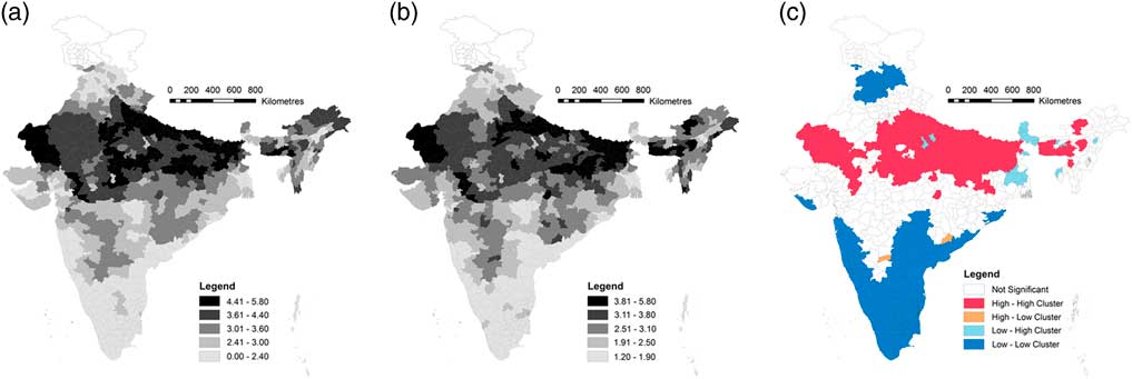
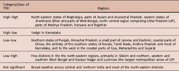
The district-level TFR maps for 2001 and 2011 (Fig. 3a and b) show higher fertility rates in north-eastern, north and central India, while the south-eastern coastal region and all the southern and south-western districts had comparatively lower fertility levels. They also revealed very little change in the district-level fertility, suggesting a slow pace of fertility transition across the country. While Moran’s I statistics showed the overall patterns of spatial autocorrelation, they did not reveal the local pattern of the spatial dependence. These were assessed through LISA statistics (Anselin, Reference Anselin1995), which explained the local spatial autocorrelation functionability and identified particular locations of spatial clusters (Fig. 3c), highlighting the prominent local patterns of spatial dependence in the district-level TFRs using a five-pronged classification scheme: high–high, high–low, low–low, low–high and ‘not significant’ districts (Table 2). Districts in the ‘not significant’ group reflected no significant autocorrelation with proximate districts, being neither outliers nor clusters (Jun, Reference Jun2017). The high–high districts were those with a high TFR that were surrounded by other high-TFR districts and similarly for the low–low class districts. The dominance of high–high and low–low clusters confirmed the overall positive spatial autocorrelation in the TFR. Besides this, there were some spatial outliers with high–low and low–high TFR combinations, which were outliers. Overall, the LISA map revealed that the TFR distribution varied significantly across space and underlined the importance of considering spatial heterogeneity in such local-level studies.
District-level TFR and the local clusters/outliers. (a) TFR (2001); (b) TFR (2011); (c) LISA TFR (2011).
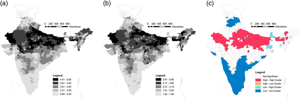
Spatial distribution of the enumerated TFR (LISA) across India’s districts
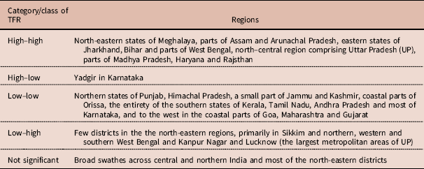
Source: compiled by the authors.
Modelling fertility rates at the district level
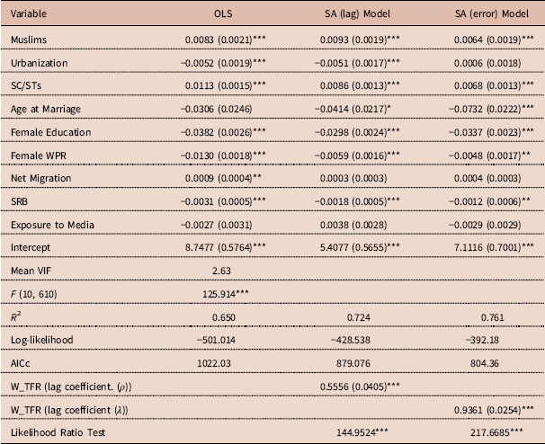
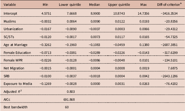
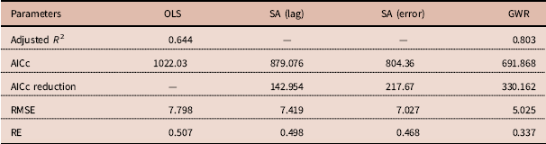
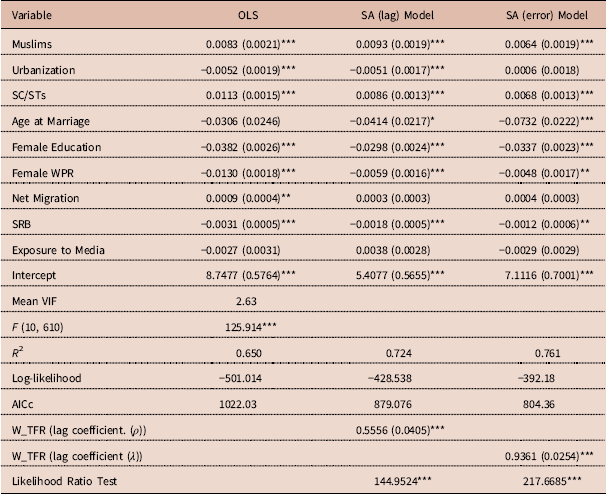
Estimations from the three models are presented in Table 3, the significant GWR local coefficients, goodness-of-fit values and standardized residual from the GWR model are displayed in Figures 5 and 6, respectively, and the summary of the GWR model and the respective performance statistics (AICc) and measures of prediction accuracy (RE and RMSE) of all the models are reported in Tables 4 and 6, respectively.
Estimates from the global OLS and spatial regressions (N=621)
Source: authors’ own calculations.
***p<0.01; **p<0.05; *p<0.1; standard errors are in the parentheses.
Estimates of the GWR local model (N=621)
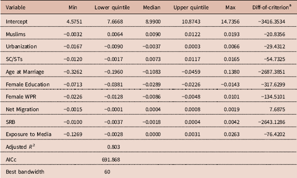
a This tests the geographical variability of local parameter estimates. A positive value indicates no geographical variability. Source: authors’ own calculations.
Global regression results
The OLS and SA (lag/error) models showed that barring Exposure to Media, the rest of the variables were statistically significant and bore the expected signs (Table 3). In particular, Muslims and SC/STs revealed highly significant positive relationships with the district-level TFR. Though Urbanization flagged a negative relationship with the TFR, it was only significant in the OLS and SA (lag) model. Among other variables, the respective negative coefficients between Age at Marriage, Female Education, Female WPR and the TFR implied that ceteris paribus, districts where access to education and female empowerment was high had low fertility levels. Net Migration had a positive relationship with the TFR but was significant only in the OLS model, suggesting that higher rates of population inflow increased the fertility rate, tallying with the surmise of Işik and Pinarcioğlu (Reference Işik and Pinarcioğlu2006). The global models revealed the SRB to have a negative relationship with the TFR, denoting that districts with a more skewed SRB (fewer female births than male births) had a higher fertility, such as in the northern Indian states.
The tests for ρ and λ (Table 3) implied that a significant autocorrelation existed among the district-level fertility rates and the error terms. A considerable difference was also shown between the aspatial OLS model and the SA (lag/error) regressions with respect to the magnitude of the β coefficient values and the SA (lag/error) models fitted the data much better. The log-likelihood values increased while the AICc decreased in the SA (lag/error) models, as compared with the OLS model.
Geographically Weighted Regression results
While the previous section revealed that the relationships between the district-level TFR and different demographic and socioeconomic parameters were as generally expected, this section discusses how the identified associations varied from one region to another and to what extent such local associations remained masked in the global regressions, through the estimated GWR local coefficients (Table 4).
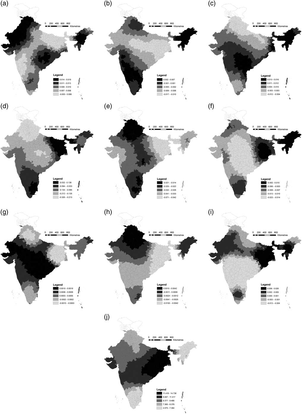
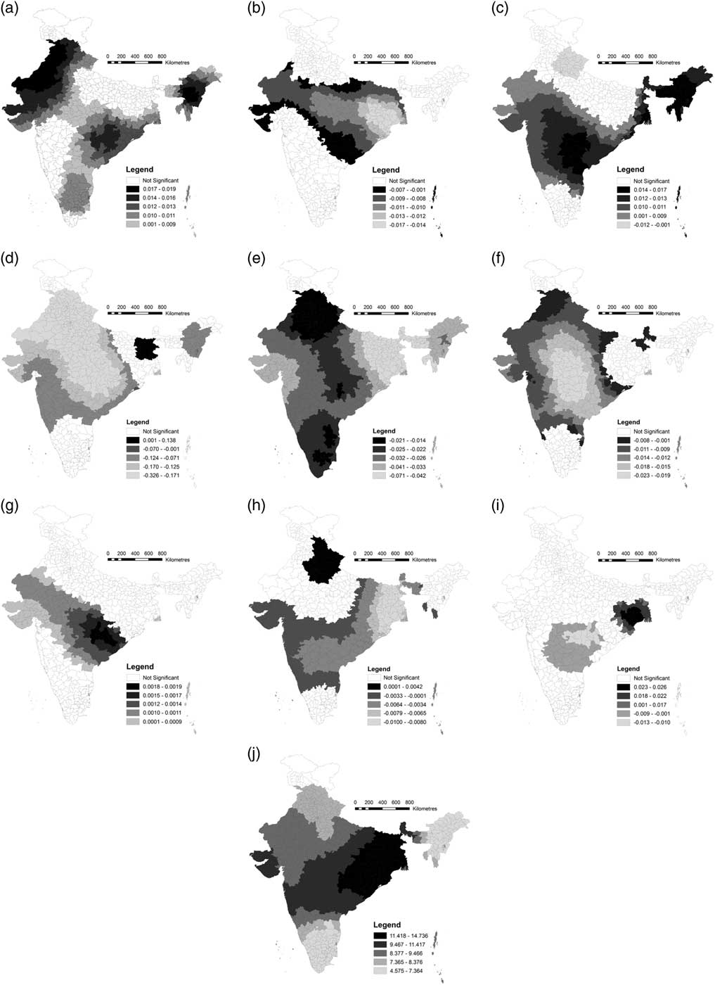
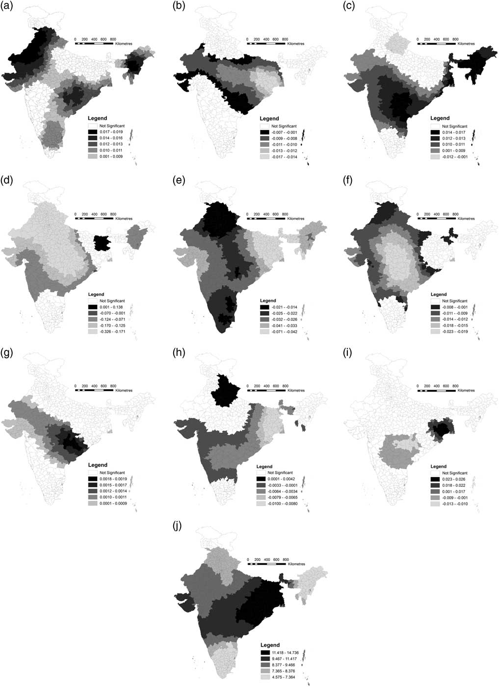
Barring Net Migration, all the independent variables were spatially non-stationary and therefore could be considered as local covariates (last column, Table 4). The GWR local coefficients of all variables statistically significant at the 5% level were mapped for a more nuanced econometric interpretation (Fig. 5). These variables have also been mapped previously without the significance levels for visual comparison (Fig. 4).
Spatial distribution of GWR local coefficients at the district level (without showing significance level). (a) Muslims; (b) Urbanization; (c) SC/STs (d) Female Mean Age at Marriage; (e) Female Education; (f) Female WPR; (g) Net Migration; (h) Sex Ratio at Birth (SRB); (i) Exposure to Media; (j) Intercept. Local coefficients are presented in quintile scales. The analysis is based on 621 districts with nineteen districts of Jammu and Kashmir excluded due to the non-availability of TFR data. Source: same as Table 1.
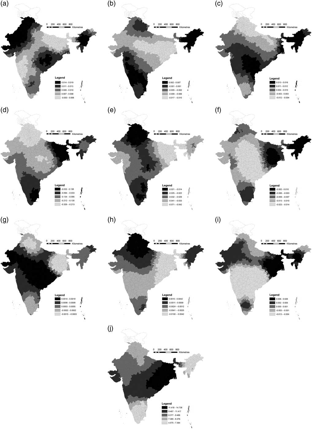
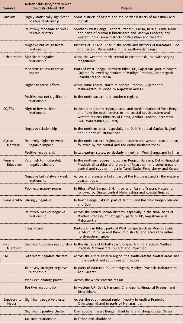
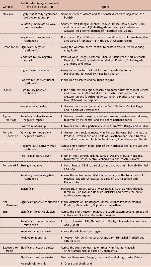
The interpretation of the local coefficients (Fig. 5) supported the initial assumption that the impacts of the select socioeconomic and demographic variables on the district-level fertility rate were not spatially invariant (i.e. not all the predictors were statistically significantly related to TFRs everywhere) and that the selected covariates imparted a significant influence on the TFRs only in specific areas of the country, with this substantially differing in terms of magnitude, direction and strength across locations (Table 5).
Spatial distribution of GWR local coefficients at the district level (significant areas only). (a) Muslims; (b) Urbanization; (c) SC/STs; (d) Female Mean Age at Marriage; (e) Female Education; (f) Female WPR; (g) Net Migration; (h) Sex Ratio at Birth (SRB); (i) Exposure to Media; (j) Intercept. All coefficients are significant at the 5% level. The classes are determined using the natural breaks scheme of Jenks (Jenks & Caspall, Reference Jenks and Caspall1971). The analysis is based on 621 districts with nineteen districts of Jammu and Kashmir excluded due to the non-availability of TFR data. Source: same as Table 1.
Spatial distribution of the local relationships between the TFR and the independent variables across India’s districts
Source: compiled by the authors.
The varying magnitude of the relationship between Muslims and TFR (Fig. 5a) implied that fertility behaviours differed reasonably even among Muslim populations, being grounded in distinct local contextual factors. A caste-based fertility differential was also conspicuous (Fig. 5c), with the relationship between SC/STs and TFR varying substantially in terms of direction, strength and magnitude across places. Districts from the north-eastern, central and south-western tribal belts of India showed a positive relationship between the SC/STs and fertility rates, primarily as in these areas the material development, degree of rural–urban interaction and pace of adaptation to changing societal norms through diffusion of ideas and information remain significantly low or had been sluggish. Contrarily, a relative higher level of social development, faster acclimatization to the urban way of life through strong diffusion channels and social interaction and the resultant increased upward mobility nullified the effect of social marginalization on fertility in the Delhi metropolitan region and its hinterland, including a part of Uttarakhand. Understandably, compared with the faster structural transformation in economic and institutional fronts, the cultural and normative shift might be delayed, thereby precipitating such reversal of causality between social marginalization and fertility behaviour across the locations, which should thus not be always surmised by overarching generalized statements. Since ethnic and socio-cultural heterogeneities remain pervasive in these three regions, especially in the north-east, which has a greater proportion of SC/STs whose cultural attributes differ markedly from those of other north or south Indians, understanding their fertility behaviour becomes quite complex.
The Urbanization to TFR relationship (Fig. 5b) was expectedly negative but was statistically significant only in some regions. Many districts flagged a moderate to low negative impact of urbanization on their TFR, especially in less-urbanized areas (e.g. many districts of Orissa) having lower economic development and poor rural–urban interactions. The Urbanization–TFR relationship was also proven to be context-specific with respect to socio-cultural norms since some regions with greater urbanization had a tenuous correlation with the TFR, though not significantly so, and this particular finding resonated strongly with that of Dreze and Murthi (Reference Dreze and Murthi2001).
The global regressions reported a negative relation between Age at Marriage and TFR (Fig. 5d), but the GWR results indicated that this did not hold over the entire country, with there being both negative and positive significant relationships, and its effect varying spatially due to highly place-specific fertility behaviour. While an increase in age at the time of marriage does reduce fertility among younger people, taken in aggregate, the effect of marriage-based factors may not be that large in some areas (Kulkarni, Reference Kulkarni2011).
The expected significant negative relationship between Female Education and TFR was found everywhere (Fig. 5e), though its magnitude differed substantially between locations – from very high to moderately negative clusters wherein female education had played a vital role in reducing the fertility level, to a negative but relatively weak relationship in some areas, unearthing a crucial dynamic. A poorer explanatory power was apparent in regions that had a lower share of females (aged 15–49 years) who had completed primary/secondary or higher education. This partly suggests that in addition to the rise in female education, some other societal norms (e.g. gender attitudes) and certain economic thresholds have to be met before fertility decline is initiated (Jain, Reference Jain1981; Wang & Chi, Reference Wang and Chi2017). Hence, future fertility reduction policies that seek to enhance female education levels need to be prioritized in socioeconomically poorer districts, since feasibly, a rise in the household socioeconomic status would translate into more girls being encouraged, or able, to carry on and further their education.
The relationship between the Female WPR and the TFR was negative (Fig. 5f), though quite varied. While most districts flagged the expected negative relationship, in some areas this was insignificant. A plausible explanation was the lower female work participation rate in the non-domestic sphere in these areas, with prevalent practices of traditional gender-based roles and family norms and lesser female empowerment. For the southern states, this narrative was probably quite different since they had already attained replacement level fertility (Kulkarni, Reference Kulkarni2011; Dharmalingam et al., Reference Dharmalingam, Rajan and Morgan2014).
The significant positive relationship between the Net Migration and TFR (Fig. 5g) was strongly location based. Significant local coefficients were only seen in select districts, leaving vast areas as statistically insignificant. Where net migration was negative (higher out-migration), fertility rates were relatively lower as feasibly mostly younger people moved away for education or employment. Conversely, in the gaining regions, primarily in Maharashtra (India’s leading in-migration state) and Gujarat, which had a net positive migration, the fertility levels were likely to rise, with new in-migrants requiring time to acclimatize to the prevalent urban fertility norms.
The global regression resulted in a negative relationship between the SRB and TFR (Fig. 5h) while the GWR local map revealed that it differed in magnitude and direction across India. Thus, all else being equal, a more balanced SRB (higher SRB) was related to a lower TFR, even though low TFRs may also skew the SRB, as found in the Nagapattinam and Puducherry districts of Tamil Nadu and Puducherry, respectively. A weak explanatory power in the eastern region may be attributed to the recent fall in the SRB in that region (Rajan et al., Reference Rajan, Srinivasan and Bedi2017). The positive SRB–TFR relationship across northern India probably resulted from: 1) a historically strong son preference/gender discrimination in these areas, 2) a much skewed SRB present there for decades, and 3) entrenched patriarchal societal norms and value systems that hinder women from taking fertility-related decisions, with its ensuing ramifications on family planning methods. Therefore, the SRB to TFR relationship was highly context-specific, encapsulating various socio-religious norms and cultural backgrounds (Das Gupta, Reference Das Gupta1987; Saha & Paul, Reference Saha and Paul2017).
The global regressions reported a negative but insignificant relationship between Exposure to Media and TFR in each district (Fig. 5i), but the local estimate revealed some interesting results with a certain paradox. As expected, its effect was not the same everywhere, differing spatially in terms of both direction and magnitude, though within limited areas, implying that this relationship was also very place-specific, as mentioned before in the context of Andhra Pradesh (see James, Reference James1999; Kulkarni, Reference Kulkarni2011; Brahmanandam & Arokiasamy, Reference Brahmanandam and Arokiasamy2016), not in the sense of the media being family planning propaganda, but rather in the perception of ‘quality living’ as depicted in popular films (Bhat, Reference Bhat1996), which was then aspired to. By contrast, a significant positive effect of media exposure on the TFR was found in Orissa, southern Jharkhand, and along the western border of West Bengal, possibly since these areas still suffered from complex poverty-related constraints (e.g. low per capita income, weak rural–urban interaction, low social development, poor women empowerment and high infant mortality) and the expected effect of media exposure may occur only after a time lag. Another possible reason could be the aforementioned threshold effect, (Jain, Reference Jain1981), as discussed previously regarding female education, but prescribing a definite threshold level for this remains difficult. Nonetheless, the reasons as to why media exposure did not exert the expected effect in this particular belt, while doing so in Andhra Pradesh and its surrounding regions, requires further in-depth analysis.
Performance assessment and prediction accuracy of the models
All the spatial models (the autoregressive lag/error and the GWR) aligned with the data more closely than the non-spatial OLS regression. Among these, the GWR provided the best fit for the data with the least AICc (691.868), while the spatial error model performed just a bit better than the spatial lag model (Table 6). Furthermore, the adjusted R 2 values showed significant improvement in the GWR estimation (R 2 GWR >R 2 OLS).
Models’ performance and prediction accuracy assessment

Abbreviations are defined in the text. Source: authors’ own calculations.
The RE and RMSE statistics showed that the GWR performed best, followed by the other spatial autoregressive models. Compared with the conventional OLS model, the local GWR model output improved the prediction accuracy by more than 35%, implying that many previously un-captured fertility determinants were strongly location-dependent. Thus, the GWR’s inherent comprehension and interpretation of the spatial heterogeneity as a natural mechanism underlying the fertility behaviour made it the best predictive model.
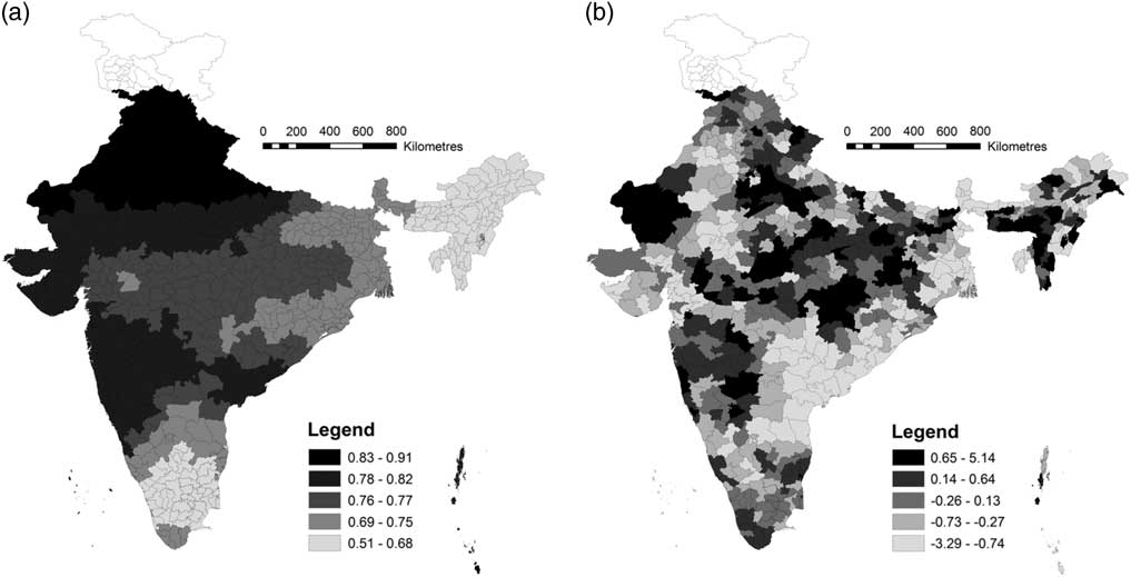
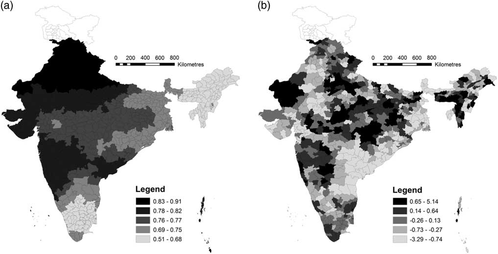
To see how the GWR best fitted the data, maps of the local R 2 (Fig. 6a) and local residual values (Fig. 6b) were prepared. The local R 2 values ranged from 0.510 to 0.910. The GWR model was a better fit in the northern, central and western parts of the country, while the north-eastern, eastern, south-eastern coastal belt and the southerns zones elicited a relatively poorer model fit, since the R 2 values were lower there in comparison to its northern counterparts. Crucially, in those areas where the low–low TFR clusters were present (see Fig. 3c), the GWR model did not fit well (e.g. in the contiguous southern states of Kerala, Tamil Nadu and Karnataka).
GWR model fits. (a) Local R 2; (b) Local standardized residual.
Conclusion
India’s district-level fertility patterns and differentials, as deciphered from the most recent Census data of 2011, can still be explained via the traditional development framework in most regions, while in select locales, the manifestation of low fertility rates may indicate newer fertility attributes distinct from those occurring during the initial phase of transition. Such regional differences may have arisen from huge variations in socioeconomic development and population policy implementation merged together with distinct local socio-cultural–religious norms and behaviour. This paper examined the spatial dynamics of such district-level fertility behaviour across India using some novel spatial econometric techniques and revealed that the relationships between the districts’ TFR and their respective demographic and socioeconomic factors were not spatially invariant, with the effect of these factors also varying in magnitude, direction and significance across the examined space. Such varying associations seldom followed predefined administrative state/UTs boundaries, implying inter- and intra-state/UT spatial variations, indicating that strong micro-regional influences could override even state-level government family planning policies and requiring them to be even more location-specific and tailor-made to address the niche resident populations of such smaller regions. Of the five proposed hypotheses earlier, four were seemingly quite well supported by the derived GWR local estimations.
First, quite expectedly, the level of economic development measured by Urbanization flagged a negative relationship with the TFR but only significantly so in the western and north–central to eastern regions and with varying magnitudes. However, no significant positive effect of economic development on the TFR was observed, suggesting that well-off parents seldom wished for more children, instead seeking a better quality of life, education and opportunities for their offspring, which was economically more feasible for smaller families. Second, many less-urbanized districts flagged a negative relationship with the TFR (e.g. in Orissa, Chhattisgarh, Jharkhand and Madhya Pradesh – primarily the central, interior belt of India), implying that rural areas should not always be regarded as high-fertility locales, since smaller (than before) family ideals have pervaded among almost all sections of society, with recent studies reporting a considerable decrease in the rural–urban fertility differential across India (Kulkarni, Reference Kulkarni2011). Third, while a significant negative relationship between Female Education and the TFR was almost universal, a relatively weak negative effect was also found across the entire eastern zone, parts of the north-east and the western coastal regions, possibly due to the continued prevalence of traditional family norms. As stated before, apart from enhancing female education, attaining other socioeconomic thresholds is thus important in initiating fertility decline, since a universally negative effect of female education on fertility rates occurs only when women have some freedom in taking childbearing decisions (Jain, Reference Jain1981; Jejeebhoy, Reference Jejeebhoy1995). Fourth, the relationships of the main religious minority group, Muslims, and the most socially marginalized caste group, SC/STs, with the TFR, were highly place-specific, showing distinct fertility patterns, based on their residence location and socio-cultural norms, which should not be always surmised by overarching generalized statements. Fifth, linkages between the diffusion of knowledge, aspirations and ideas on fertility preferences and lifestyles with the fertility rate were region- and context-specific, and at times quite puzzling. As such, both significant negative and positive effects of Exposure to Media on the TFR were found, though only in some regions, highlighting the place-specificity of its influence, similar to that posited by Kulkarni (Reference Kulkarni2011) and requiring further research. Sixth, consistent with the existing literature, this paper asserts that the prevailing demographic and socioeconomic factors exerted low explanatory power in districts where significant clusters of low fertility rates existed (Wang & Chi, Reference Wang and Chi2017). The LISA map (Fig. 3c) displayed two different zones with spatial clusters of low-fertility rates (Table 2) and the GWR results revealed better model performance in the northern zone but not as well in the southern region (Fig. 6a). The selected nine explanatory variables could neither fully, nor in a comparatively better way, explain the clusters of low TFRs in the southern region, indicating that possibly other socioeconomic–demographic parameters not considered in this study, were operative in precipitating such low-fertility clusters in this region. Therefore the models used for such analyses may also themselves need to be more location-specific.
For a vast country like India, thus, it is possible and seemingly more apt that region-specific fertility models (i.e. different models considering different parameters for explaning fertility trends of specific locales) are more suitable than a national-level overarching hypothesis, with this bearing on important policy decisions in terms of where, what and how to address, while trying to influence reproductive behaviour and decline population growth. This is imperative as this study reveals fertility behaviour to be highly context- and place-specific, whose variations cannot be explained by a single narrative of either socioeconomic advancement or government intervention. Given that marked spatial variations in fertility rates (and their future trend predictions of persistence or convergence) remain a critical issue while carrying out national/sub-national-level population projections, these findings can thus be quite useful in policy framing as inter-district fertility differentials would have vital implications for local-level decentralized planning towards providing family planning, health care, education and other welfare services.
This paper has a few caveats that should be noted. Census-based fertility estimations were used, which may suffer from measurement errors stemming from misreporting (under-/over-reporting) of births. This measurement error issue could have been less problematic if the errors had been spatially homogeneous and uncorrelated with any explanatory variables. Occurrences of birth misreporting can be more prevalent in certain socio-politically-sensitive areas (e.g. Jammu and Kashmir – for a review, see Guilmoto & Rajan, Reference Guilmoto and Rajan2013). Usually, such mis(under)reporting of births is more frequent in rural areas than in urban locales and more likely in the case of a girl child than for boys (Guilmoto et al., Reference Guilmoto, Saikia, Tamrakar and Bora2018). If such be the case, then it is possible that the coefficient that was estimated for the SRB was seemingly biased downward. Furthermore, since reliable estimations of the SRB are seldom available at the district level from the Sample Registration System (SRS) in India, it was computed from the relevant census data on recent births, which may not be perfectly reliable. The net migration rate was also computed from previous census data (of 2001) as the most recent migration data from the 2011 Census are yet to be published. These potential data limitations and their ensuing measurement issues are hereby acknowledged. Allied to this, the analyses of only a few parameters, solely based on the census databases, also restrict the paper by precluding the incorporation of more accurate measures of economic development (e.g. GDP per capita/household level income) and other vital predictors of the TFR level (e.g. child mortality rate: Işik & Pinarcioğlu, Reference Işik and Pinarcioğlu2006; Das & Mohanty, Reference Das and Mohanty2012).
Notwithstanding these lacunae, this detailed nationwide study has elicited some interesting and new insights into the spatial dimensions of fertility differentials in India, having examined its dynamics through a district-level geocoded database. It has also highlighted the importance of considering locational aspects in fertility research through the GWR method, which enables the modelling of spatial variations in a more intuitive manner as compared with the conventional global model, in terms of both model performance and prediction accuracy. It is hoped that this paper shall spur further research to examine the trajectories of change in these spatial factors that influence fertility transitions over time, as well as their respective trends across the board, using longitudinal data. Such further insights would certainly provide policymakers and demographers with a holistic understanding of the interplay of causative factors that influence the fertility transition processes within and across areas.
Acknowledgments
The authors are grateful to the two anonymous reviewers whose invaluable comments and suggestions helped in improving this article substantially. The authors are also indebted to Rakesh Mishra and Md Juel Rana, both PhD candidates at the Centre for the Study of Regional Development, Jawaharlal Nehru University, New Delhi, India, for their comments on an earlier draft of the manuscript. All remaining errors, if any, are those of the authors themselves.
Ethical Approval
The authors assert that all procedures contributing to this work comply with the ethical standards of the relevant national and institutional committees on human experimentation and with the Helsinki Declaration of 1975, as revised in 2008.
Conflicts of Interest
The authors have no conflicts of interest to declare.
Funding
This research received no specific grant from any funding agency, commercial entity or not-for-profit organization.