3.1 Mean statistics

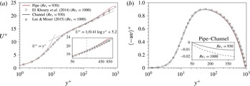
Figure 1(a) plots the mean streamwise velocity profiles of the pipe and channel flows at $\mathit{Re}_{\unicode[STIX]{x1D70F}}\approx 930$ . The available DNS data of the pipe (El Khoury et al. Reference El Khoury, Schlatter, Brethouwer and Johansson2014) and channel (Lee & Moser Reference Lee and Moser2015) flows at $\mathit{Re}_{\unicode[STIX]{x1D70F}}\approx 1000$ are included for comparison. Although the present mean velocity profiles lie above the reference data in the wake region due to relatively strong pressure gradient (low Reynolds number), the following trends are analogous in the pipe and channel flows; the validation with similar Reynolds numbers is provided in Ahn et al. (Reference Ahn, Lee, Jang and Sung2013) and Lee et al. (Reference Lee, Lee, Choi and Sung2014). The mean velocity profiles of the internal flows expressed in terms of wall units coincide below $y^{+}\approx 150$ ( $y/\unicode[STIX]{x1D6FF}\approx 0.15$ ). Above this location, a discrepancy is observed between two profiles; the mean velocity of the pipe flow is higher than that of the channel flow. Although such a difference in the wake region was reported by several investigators e.g. Monty et al. (Reference Monty, Hutchins, Ng, Marusic and Chong2009) and El Khoury et al. (Reference El Khoury, Schlatter, Brethouwer and Johansson2014), the underlying cause of this difference has not yet been understood. Nieuwstadt & Bradshaw (Reference Nieuwstadt, Bradshaw, Henkes and Bakker1997) conjectured that the discrepancy in the core region could arise from a different spanwise (azimuthal) space: the available space is reduced to zero toward the pipe centre. On the other hand, the lower mean velocity of the channel flow leads to a smaller wall-normal gradient than that of the pipe flow, owing to the strong wake component ( $y^{+}\,\text{d}U^{+}/\text{d}y^{+}$ ) in the pipe flow. Chin et al. (Reference Chin, Monty and Ooi2014a ) suggested that the discrepancy in the wake component is presumably correlated to the structural differences in the core region. These previous studies support the idea that the mean flow in the pipe and channel flows is different and there is a possible connection between the mean flow and the flow structure.

The profiles of the Reynolds shear stress $\langle -uv\rangle ^{+}$ in the pipe and channel flows are shown in figure 1(b). The profiles collapse well up to the peak position $y_{p}^{+}\approx 53$ , however, a slight difference is displayed above this peak. An enlarged view in the inset of figure 1(b) shows the difference in $\langle -uv\rangle ^{+}$ between the pipe and channel flows; the negative value indicates a lower $\langle -uv\rangle ^{+}$ for the pipe flow. Above $y_{p}^{+}$ , a difference in $\langle -uv\rangle ^{+}$ between the channel and pipe flows appears and increases continuously up to $y/\unicode[STIX]{x1D6FF}\approx 0.5$ , where the mean shear ( $\text{d}U/\text{d}y$ ) of the channel flow is slightly lower than that of the pipe flow in figure 1(a).

Figure 1.

Wall-normal distributions of (a) the streamwise mean velocity and (b) the Reynolds shear stress. Red and black lines indicate the present pipe and channel flows at $\mathit{Re}_{\unicode[STIX]{x1D70F}}\approx 930$ , respectively. Vertical dashed line in the inset of (a) is at $y^{+}=150$ . The inset of (b) shows the difference in the Reynolds shear stress, $\langle -uv\rangle _{pipe}^{+}-\langle -uv\rangle _{channel}^{+}$ .

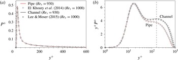
Next, the production of TKE ( $P$ ), which is the product of $\text{d}U/\text{d}y$ and $\langle -uv\rangle$ is shown in figure 2(a). The physical meaning of the production is that the action of the mean shear working against the Reynolds shear stress extracts kinetic energy from the mean flow and transfers it to the fluctuating velocity field for sustaining the turbulence. The profile of $P^{+}$ collapses well in the internal flows. However, it should be noted that the semi-log plot of $P$ does not reveal its contribution to the bulk production (Marusic, Mathis & Hutchins Reference Marusic, Mathis and Hutchins2010). A premultiplication is required to represent the contribution to the integral of $P$ when the abscissa is in a logarithmic scale (figure 2 b). Note that the premultiplication for the pipe flow includes two terms; one is the integration along $y^{+}$ , the other is the axial distance $r$ . In the overlap region, the premultiplied production of the channel flow has a larger magnitude than that of the pipe flow. The latter drops rapidly in the core region, revealing that the overlap region contributes to the bulk production more strongly in the channel flow than in the pipe flow. In addition, an outer peak is observed at $y^{+}\approx 160$ in the channel flow. Marusic et al. (Reference Marusic, Mathis and Hutchins2010) reported that the contribution of the overlap region to the overall turbulence production increases with increasing the Reynolds number. This observation implied a growing role of the LSMs in producing turbulence as the Reynolds number increases. Thus, the discrepancy of the premultiplied $P$ in the overlap region could be related to the different contributions of LSMs between the pipe and channel flows As addressed in the Introduction, the turbulent inertia is the Reynolds shear stress force which accelerates or decelerates the mean velocity (i.e. influence on the mean velocity gradient). To further investigate the difference observed in the TKE production, it is valuable to examine the contributions of LSMs and their roles in terms of the turbulent inertia.

Figure 2.

Wall-normal distributions of (a) $P^{+}$ and (b) the premultiplied production normalized by viscous wall units. The inserted vertical line in figure 2(b) indicates an outer peak of the channel flow at $y^{+}=160$ .

3.2 Spectral density function

3.2.1 Spectra of the Reynolds shear stress and turbulent kinetic energy production

The scales that contribute to the difference in the turbulent statistics are explored by analysing the spectral density function $(\unicode[STIX]{x1D6F7})$ . The co-spectrum of $u$ and $v$ is expressed by

(3.1) $$\begin{eqnarray}\langle -uv\rangle (y)=\int _{0}^{\infty }\unicode[STIX]{x1D6F7}_{-uv}(k_{x},y)\,\text{d}k_{x},\end{eqnarray}$$

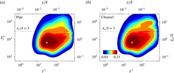
which indicates that $\unicode[STIX]{x1D6F7}_{-uv}$ represents the spectral contribution to $\langle -uv\rangle$ and $k_{x}$ is the streamwise wavenumber. We first explore the premultiplied streamwise spectra of the Reynolds shear stress to examine the difference in the premultiplied TKE production (figure 2 b) because $P$ is the production of turbulent energy by the Reynolds shear stress. The premultiplied streamwise spectra of the Reynolds shear stress, $k_{x}\unicode[STIX]{x1D6F7}_{-uv}^{+}$ is shown in figure 3. The inner energy site of the spectra, which is associated with the near-wall cycle (Jiménez & Pinelli Reference Jiménez and Pinelli1999; Schoppa & Hussain Reference Schoppa and Hussain2002), is located at $y^{+}\approx 30$ and $\unicode[STIX]{x1D706}_{x}^{+}\approx 700$ (marked by ‘ $+$ ’). The wall-normal location of the inner energy site is further from the wall than it is in the spectrum of the streamwise velocity fluctuations ( $y^{+}\approx 15$ ) due to the attenuation of the wall-normal velocity fluctuations in the near-wall region (Wu et al. Reference Wu, Baltzer and Adrian2012).

Figure 3.

Premultiplied streamwise spectra of the Reynolds shear stress, $k_{x}\unicode[STIX]{x1D6F7}_{-uv}^{+}$ , in (a) pipe and (b) channel flows at $\mathit{Re}_{\unicode[STIX]{x1D70F}}\approx 930$ . The inserted horizontal line indicates at $\unicode[STIX]{x1D706}_{x}/\unicode[STIX]{x1D6FF}=3$ . The cross symbol represents the inner site at $y^{+}\approx 30$ and $\unicode[STIX]{x1D706}_{x}^{+}\approx 700$ .

Although the values of $k_{x}\unicode[STIX]{x1D6F7}_{-uv}^{+}$ in the near-wall region are similar in the pipe and channel flows, the spectral contributions in the outer region differ significantly. Both spectra show protrusions at the longer wavelengths ( $\unicode[STIX]{x1D706}_{x}>3\unicode[STIX]{x1D6FF}$ ) over the range $0.1<y/\unicode[STIX]{x1D6FF}<0.3$ , implying that the outer peak could appear at higher Reynolds numbers (Wu et al. Reference Wu, Baltzer and Adrian2012). Recently, Ahn et al. (Reference Ahn, Lee, Lee, Kang and Sung2015) reported that the outer energy peak in the $\langle -uv\rangle$ spectrum is located at $y/\unicode[STIX]{x1D6FF}=0.173$ and $\unicode[STIX]{x1D706}_{x}/\unicode[STIX]{x1D6FF}=10$ , using the DNS of turbulent pipe flow at $\mathit{Re}_{\unicode[STIX]{x1D70F}}=3000$ . Although no outer peak is observed in the present DNS data, the protrusions observed in this range could form the outer energy site observed in Ahn et al. (Reference Ahn, Lee, Lee, Kang and Sung2015). The protrusions shown in figure 3 suggest that the longer wavelength contributes predominantly to $k_{x}\unicode[STIX]{x1D6F7}_{-uv}^{+}$ in the outer region. A bulge-like shape is prominent in the channel flow. At the longer wavelengths ( $\unicode[STIX]{x1D706}_{x}/\unicode[STIX]{x1D6FF}>3$ ), in particular, the spectral contribution to $\langle -uv\rangle$ in the channel flow exceeds that that of the pipe flow, indicating that the long-wavelength motions transfer more momentum in the outer region of the channel flow than in the pipe flow. The discrepancy between the co-spectra is attributed to the slight difference in the $\langle -uv\rangle$ profile shown in figure 1(b).

The difference observed in the profile of premultiplied TKE production (figure 2 b) which could be related to the different contributions of the LSMs, is explored by examining the streamwise spectrum of the production. The spectrum of the production is

(3.2) $$\begin{eqnarray}P(y)=\int _{0}^{\infty }\unicode[STIX]{x1D6F7}_{P}(k_{x},y)\,\text{d}k_{x},\end{eqnarray}$$

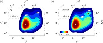
where the production spectrum $\unicode[STIX]{x1D6F7}_{P}(k_{x},y)$ is given by the product of the mean velocity gradient and the Reynolds shear stress spectrum. Figure 4 displays a contour map of the spectrum of the TKE production ( $P$ ) multiplied by the wall-normal distance and wavenumber, $y^{+}k_{x}\unicode[STIX]{x1D6F7}_{P}^{+}$ . Equal areas under the spectrum map represent equal contributions to the integral. The inner peak (marked by a white cross symbol) in the spectrum at $y^{+}\approx 15$ is consistent with the peak location of $P^{+}$ in figure 2. Note that the streamwise wavelength of the inner peak is located at $\unicode[STIX]{x1D706}_{x}^{+}\approx 660$ , similar to the inner site in $k_{x}\unicode[STIX]{x1D6F7}_{-uv}^{+}$ (figure 3), indicating that the small scales predominantly contribute to the production of TKE and the momentum transfer in the near-wall region. In the outer region, however, the spectrum of the channel flow shows a different form compared to that of the pipe flow. In figure 4(a), a ridge is observed in the core region while there is a weak peak (indicated by a black cross symbol) located at $y/\unicode[STIX]{x1D6FF}\approx 0.28$ and $\unicode[STIX]{x1D706}_{x}/\unicode[STIX]{x1D6FF}\approx 8$ in (b); the 0.4 contour line represents the outer site in the channel flow. The vertical line indicates $y^{+}=160$ , the position of the outer peak in the profile of the premultiplied production in figure 2(b). Since the integral of $y^{+}k_{x}\unicode[STIX]{x1D6F7}_{P}^{+}$ over whole wavelengths is equal to the quantity of $y^{+}P^{+}$ , the emergence of the outer peak in the channel flow (figure 2 b) arises from the long-wavelength motions. In the overlap region, moreover, an inner hump is observed in the 0.3 and 0.4 contour lines of the pipe flow, whereas the contour lines of the channel flow in the same range show a relatively weak inner hump compared to the pipe flow. Owing to the dominant effects of the longer wavelengths in the channel flow, the discrepancy in the overlap region contribution to the bulk production (figure 2 b) appears, even though the friction Reynolds numbers are equal for the pipe and channel flows. Therefore, the present spectrum analysis clarifies the different contributions of large scales to the momentum transfer and the production of TKE in internal flows.

Figure 4.

Streamwise spectra of the production of turbulent kinetic energy premultiplied by the wall-normal distance and wavenumber, $y^{+}k_{x}\unicode[STIX]{x1D6F7}_{P}^{+}$ , in (a) pipe and (b) channel flows at $\mathit{Re}_{\unicode[STIX]{x1D70F}}\approx 930$ . The inserted vertical lines indicate at $y^{+}=160$ ( $y/\unicode[STIX]{x1D6FF}=0.17$ ) and the horizontal line indicates at $\unicode[STIX]{x1D706}_{x}/\unicode[STIX]{x1D6FF}=3$ . The white cross symbol represents the inner site at $y^{+}\approx 15$ and $\unicode[STIX]{x1D706}_{x}^{+}\approx 660$ and the black cross symbol indicates the outer site of the channel flow at $y/\unicode[STIX]{x1D6FF}\approx 0.28$ and $\unicode[STIX]{x1D706}_{x}/\unicode[STIX]{x1D6FF}\approx 8$ . The contours are varied from 0.1 to 0.9 with an increment of 0.1.

3.2.2 Net force spectra

The wall-normal derivative of the Reynolds shear stress (turbulent inertia), $\unicode[STIX]{x2202}\langle -uv\rangle /\unicode[STIX]{x2202}y$ , is the net Reynolds force whose effects on the mean flow are much easier to understand than the Reynolds stress (Wu et al. Reference Wu, Baltzer and Adrian2012). In addition, the spectrum of the net Reynolds force presents the roles of different eddy scales that influence the mean flow by accelerating or decelerating the flow. Hence, the net force spectrum is examined to further investigate the role of LSMs which are dominant contributors of the momentum transport and of producing kinetic energy in the channel flow.

Figure 5.

Premultiplied streamwise spectra of the turbulent inertia, $k_{x}\unicode[STIX]{x2202}\unicode[STIX]{x1D6F7}_{-uv}^{+}/\unicode[STIX]{x2202}y^{+}$ , in (a) pipe and (b) channel flows at $\mathit{Re}_{\unicode[STIX]{x1D70F}}=930$ . The line contours indicate $k_{x}\unicode[STIX]{x2202}\unicode[STIX]{x1D6F7}_{-uv}^{+}/\unicode[STIX]{x2202}y^{+}=0.0004$ , 0.0006 and 0.0008. The vertical dashed lines indicate at $y^{+}=30$ and $y/\unicode[STIX]{x1D6FF}=0.15$ and the horizontal lines are at $\unicode[STIX]{x1D706}_{x}^{+}=300$ and $\unicode[STIX]{x1D706}_{x}/\unicode[STIX]{x1D6FF}=3$ . The vertical dashed-dot line marks $y^{+}=y_{p}^{+}$ .

The contributions from the streamwise wavelengths to the turbulent inertia is expressed as

(3.3) $$\begin{eqnarray}\frac{\text{d}\langle -uv\rangle }{\text{d}y}=\int _{0}^{\infty }\frac{\unicode[STIX]{x2202}\unicode[STIX]{x1D6F7}_{-uv}(k_{x},y)}{\unicode[STIX]{x2202}y}\,\text{d}k_{x},\end{eqnarray}$$

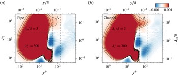
where $\unicode[STIX]{x2202}\unicode[STIX]{x1D6F7}_{-uv}/\unicode[STIX]{x2202}y$ is the net force spectrum which is the wall-normal derivative of the Reynolds shear stress spectrum. Figure 5 shows the premultiplied net force spectrum ( $k_{x}\unicode[STIX]{x2202}\unicode[STIX]{x1D6F7}_{-uv}^{+}/\unicode[STIX]{x2202}y^{+}$ ). The positive and negative regions represent the contributions to the momentum source (acceleration) and sink (deceleration) motions. The net force spectra of the pipe and channel flow are similar, and the momentum source and sink motions are dominant in the near-wall and outer regions, respectively. However, the acceleration motions of the channel flow are stronger than those of the pipe flow in the range between $\unicode[STIX]{x1D706}_{x}/\unicode[STIX]{x1D6FF}>3$ and $30<y^{+}<0.15\unicode[STIX]{x1D6FF}^{+}$ identified by A in the contour maps. The net force spectrum of the channel flow reveals a distinct ridge shape located in the overlap region, as highlighted by the contour lines in figure 5. By comparing the contour line ( $k_{x}\unicode[STIX]{x2202}\unicode[STIX]{x1D6F7}_{-uv}^{+}/\unicode[STIX]{x2202}y^{+}=0.004$ ), that of the channel flow significantly protrudes and reaches $y/\unicode[STIX]{x1D6FF}=0.15$ . Note that previous studies (Wu et al. Reference Wu, Baltzer and Adrian2012; Chin et al. Reference Chin, Philip, Klewicki, Ooi and Marusic2014b ) examined the net force spectra in the pipe flow and explained each positive or negative region in detail. The present study focuses on region A, which shows apparently different spectral behaviours in the pipe and channel flows. A comparison with figure 3 shows that the region in which the protrusion is observed in the $\langle -uv\rangle$ spectrum corresponds to the positive region of $k_{x}\unicode[STIX]{x2202}\unicode[STIX]{x1D6F7}_{-uv}^{+}/\unicode[STIX]{x2202}y^{+}$ identified as A. Because the net force spectrum is the wall-normal derivative of the co-spectrum of $\langle -uv\rangle$ , the positive value of $k_{x}\unicode[STIX]{x2202}\unicode[STIX]{x1D6F7}_{-uv}^{+}/\unicode[STIX]{x2202}y^{+}$ appears as the intensity of the $\langle -uv\rangle$ spectrum increases with  $y$ .

Although the streamwise domain length was relatively short, Chin et al. (Reference Chin, Philip, Klewicki, Ooi and Marusic2014b ) found a growth of region A (acceleration motion in the overlap region) with increasing $\mathit{Re}_{\unicode[STIX]{x1D70F}}$ . They observed that the cutoff wavelength $\unicode[STIX]{x1D706}_{x}/\unicode[STIX]{x1D6FF}=3$ , which demarcated the acceleration and deceleration motions in the overlap region used in the pipe flow ( $\mathit{Re}_{\unicode[STIX]{x1D70F}}=685$ ) of Wu et al. (Reference Wu, Baltzer and Adrian2012), was not valid at $\mathit{Re}_{\unicode[STIX]{x1D70F}}=2000$ due to the increase of region A. Chin et al. (Reference Chin, Philip, Klewicki, Ooi and Marusic2014b ) suggested that the inner normalized wavelength $\unicode[STIX]{x1D706}_{x}^{+}=3000$ was suitable to differentiate the acceleration and deceleration motions. The Reynolds number in figure 5 is approximately $\mathit{Re}_{\unicode[STIX]{x1D70F}}\approx 1000$ where $\unicode[STIX]{x1D706}_{x}^{+}=3000=3\unicode[STIX]{x1D6FF}^{+}$ . The strong LSAMs in the channel flow, even $\mathit{Re}_{\unicode[STIX]{x1D70F}}$ is consistent with the pipe flow, imply that an enhancement of region A might be more prominent in the channel flow than in the pipe flow at higher $\mathit{Re}_{\unicode[STIX]{x1D70F}}$ .

The peak values of $\langle -uv\rangle$ for both the pipe and channel flows coincide where the turbulent inertia $\text{d}\langle -uv\rangle /\text{d}y$ is zero, even though the accelerating motions differ at this wall-normal location. The vertical dashed-dot line indicates the peak location of $\langle -uv\rangle$ , $y_{p}^{+}\approx 53$ , so the integral of the net force spectra over all wavelengths along this line equals to zero. This line traverses the negative region between $300<\unicode[STIX]{x1D706}_{x}^{+}<3\unicode[STIX]{x1D6FF}^{+}$ and the positive region A. Very short wavelengths ( $\unicode[STIX]{x1D706}_{x}^{+}<300$ ) contribute negligibly due to the sign change at $y^{+}=y_{p}^{+}$ . In other words, the net force balance at $y^{+}=y_{p}^{+}$ is established between the LSAMs ( $\unicode[STIX]{x1D706}_{x}/\unicode[STIX]{x1D6FF}>3$ ) and small-scale deceleration motions ( $300<\unicode[STIX]{x1D706}_{x}^{+}<3\unicode[STIX]{x1D6FF}^{+}$ ). Thus, the same peak location of $\langle -uv\rangle$ between the pipe and channel flows indicates that the contributions of the deceleration motions in the channel flow exceed the corresponding contributions in the pipe flow to counter-balance the LSAMs. Overall, the distinct outer site observed in the channel flow in figures 3 and 4 arises from the LSMs ( $\unicode[STIX]{x1D706}_{x}/\unicode[STIX]{x1D6FF}>3$ ), which act as the momentum sources in the overlap region. Equivalently, the momentum sinks associated with the short-wavelength motions ( $300<\unicode[STIX]{x1D706}_{x}^{+}<3\unicode[STIX]{x1D6FF}^{+}$ ) dominate in the channel flow.

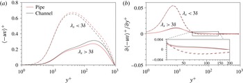
In order to quantify the contributions of LSAMs to $\langle -uv\rangle ^{+}$ and $\text{d}\langle -uv\rangle ^{+}/\text{d}y^{+}$ , these quantities are decomposed into small and large scales. Here, we choose a cutoff wavelength of $\unicode[STIX]{x1D706}_{x}=3\unicode[STIX]{x1D6FF}$ because the wavelength of the channel flow in this range displays noticeable contributions and dominantly accelerates the mean flow. Note that a more reliable cutoff wavelength is required when examining a wide range of Reynolds numbers. Figure 6(a,b) show the scale decomposition of $\langle -uv\rangle ^{+}$ and $\text{d}\langle -uv\rangle ^{+}/\text{d}y^{+}$ . Dashed and solid lines indicate the contributions of the small and large scales, respectively. In figure 6(a), the contribution of the small scales ( $\unicode[STIX]{x1D706}_{x}<3\unicode[STIX]{x1D6FF}$ ) in the channel flow is relatively low, whereas the contribution of the large scales, ( $\unicode[STIX]{x1D706}_{x}>3\unicode[STIX]{x1D6FF}$ ) is greater in the channel flow than that in the pipe flow. An outer peak ( $y^{+}\approx 200$ ) is observed in the profiles of the large-scale contributions, although the large-scale contributions at this wall-normal location are 41.7 % and 36.5 % of the total $\langle -uv\rangle ^{+}$ in the channel and pipe flows, respectively. Thus, the slight difference between the total $\langle -uv\rangle ^{+}$ in the pipe and channel flows (figure 1 b) is mainly due to the large scales ( $\unicode[STIX]{x1D706}_{x}>3\unicode[STIX]{x1D6FF}$ ) in the outer region of the channel flow. The mean fractions of $\langle -uv\rangle ^{+}$ , averaged over the wall-normal distance, are 66.5 % (small scales) and 33.5 % (large scales) in the pipe flow which are similar with the previous works (Wu et al. Reference Wu, Baltzer and Adrian2012; Chin et al. Reference Chin, Philip, Klewicki, Ooi and Marusic2014b ). On the other hand, the large scales in the channel flow account for 40.6 % of $\langle -uv\rangle ^{+}$ , which is much greater than that of the pipe flow.

The contributions of both small and large scales to $\text{d}\langle -uv\rangle ^{+}/\text{d}y^{+}$ are similar across the wall-normal direction in figure 6(b). However, the inset of figure 6(b), which is a magnified view in the region $30<y^{+}<200$ , displays a meaningful difference between the pipe and channel flows. Although the differences in the profiles of the small and large scales are relatively low, the zero crossing of $\text{d}\langle -uv\rangle ^{+}/\text{d}y^{+}$ is sensitive to the small difference. The profiles of the large scales are positive, whereas the profile of the channel flow lies above that of the pipe flow due to the dominant LSAMs (figure 5). This positive net force induced by the LSAMs balances with the retardation force of the small scales at $y^{+}=y_{p}^{+}$ . The profiles of the small scales become negative above $y^{+}\approx 40$ . In particular, the profile of the channel flow lies below the pipe flow, indicating that the similar peak location of $\langle -uv\rangle ^{+}$ between the pipe and channel flows is a result of the cancellation of the LSAMs effect in the channel flow by the strong decelerating motions of the small scales. Because the contribution of the large scales to $\text{d}\langle -uv\rangle ^{+}/\text{d}y^{+}$ increases with respect to the Reynolds number, while the profiles of the small scales collapse (Chin et al. Reference Chin, Philip, Klewicki, Ooi and Marusic2014b ), the role of the LSAMs on the outward movement of $y_{p}^{+}$ differs between the pipe and channel flows.

Figure 6.

Scale decomposition of (a) $\langle -uv\rangle ^{+}$ and (b) $\text{d}\langle -uv\rangle ^{+}/\text{d}y^{+}$ for the pipe (red) and channel (blue) flows. The dashed and solid lines represent $\unicode[STIX]{x1D706}_{x}<3\unicode[STIX]{x1D6FF}$ and $\unicode[STIX]{x1D706}_{x}>3\unicode[STIX]{x1D6FF}$ , respectively.

3.2.3 Co-spectra of the velocity–vorticity correlations

The turbulent inertia in the fully developed internal flows could be decomposed in terms of velocity–vorticity correlations according to the Stokes–Helmholtz decomposition (see Tennekes & Lumley Reference Tennekes and Lumley1972)

(3.4) $$\begin{eqnarray}\frac{\text{d}\langle -uv\rangle }{\text{d}y}=\langle v\unicode[STIX]{x1D714}_{z}\rangle +\langle -w\unicode[STIX]{x1D714}_{y}\rangle .\end{eqnarray}$$

The first term $\langle v\unicode[STIX]{x1D714}_{z}\rangle$ is related to advective vorticity transport (vorticity dispersion) whereas the second term $\langle -w\unicode[STIX]{x1D714}_{y}\rangle$ is associated with change-of-scale effect (Tennekes & Lumley Reference Tennekes and Lumley1972). In other words, the peak of the Reynolds shear stress, at which the turbulent inertia crosses the zero, indicates a balance between the two terms. The momentum source or acceleration motion is governed by the vorticity stretching $(|\langle v\unicode[STIX]{x1D714}_{z}\rangle |<|\langle w\unicode[STIX]{x1D714}_{y}\rangle |)$ in $y^{+}<y_{p}^{+}$ , whereas the momentum sink is characterized by the advective transport $(|\langle v\unicode[STIX]{x1D714}_{z}\rangle |>|\langle w\unicode[STIX]{x1D714}_{y}\rangle |)$ in $y^{+}>y_{p}^{+}$ . In this respect, the velocity–vorticity interactions are important for producing the motions that accelerate or decelerate the mean flow which is related to the momentum transport. Note that the profiles of $\langle v\unicode[STIX]{x1D714}_{z}\rangle$ and $\langle -w\unicode[STIX]{x1D714}_{y}\rangle$ are similar between the present pipe and channel flows (not shown here). Hence, the spectra of $\langle v\unicode[STIX]{x1D714}_{z}\rangle$ and $\langle -w\unicode[STIX]{x1D714}_{y}\rangle$ are explored to determine which terms dominantly influence the difference of the turbulent inertia in the overlap regions of the pipe and channel flows.

Figure 7.

Contours of the premultiplied co-spectra (a,c) $k_{x}\unicode[STIX]{x1D6F7}_{v\unicode[STIX]{x1D714}_{z}}^{+}$ and (b,d) $k_{x}\unicode[STIX]{x1D6F7}_{w\unicode[STIX]{x1D714}_{y}}^{+}$ . The filled contours change from $-0.003$ (blue) to 0.003 (red). The line contours indicate $k_{x}\unicode[STIX]{x1D6F7}_{v\unicode[STIX]{x1D714}_{z}}=-0.0009$ and $k_{x}\unicode[STIX]{x1D6F7}_{w\unicode[STIX]{x1D714}_{y}}=0.0003$ , 0.0006 and 0.0009. The vertical dashed lines correspond to $y^{+}=30$ and $y/\unicode[STIX]{x1D6FF}=0.15$ and the horizontal lines correspond to $\unicode[STIX]{x1D706}_{x}^{+}=300$ and $\unicode[STIX]{x1D706}_{x}/\unicode[STIX]{x1D6FF}=3$ . The vertical dashed-dot line marks $y^{+}=y_{p}^{+}$ .

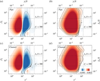
Figure 7 shows a contour map of the premultiplied co-spectra $k_{x}\unicode[STIX]{x1D6F7}_{v\unicode[STIX]{x1D714}_{z}}^{+}$ , and $k_{x}\unicode[STIX]{x1D6F7}_{-w\unicode[STIX]{x1D714}_{y}}^{+}$ . The sum of velocity–vorticity co-spectra coincides with the net force spectra in figure 5. The spectrum of $k_{x}\unicode[STIX]{x1D6F7}_{v\unicode[STIX]{x1D714}_{z}}^{+}$ changes sign from positive to negative at $y^{+}\approx 9$ , whereas the sign of $k_{x}\unicode[STIX]{x1D6F7}_{-w\unicode[STIX]{x1D714}_{y}}^{+}$ is positive in the near-wall region. Although $k_{x}\unicode[STIX]{x1D6F7}_{-w\unicode[STIX]{x1D714}_{y}}^{+}$ is significantly weakened above $y^{+}=30$ , a positive contribution of $k_{x}\unicode[STIX]{x1D6F7}_{-w\unicode[STIX]{x1D714}_{y}}^{+}$ in the long streamwise wavelength ( $\unicode[STIX]{x1D706}_{x}>3\unicode[STIX]{x1D6FF}$ ) is observed. The LSAMs result from the contribution of $\langle -w\unicode[STIX]{x1D714}_{y}\rangle$ related to the change-of-scale effect due to vortex stretching (Chin et al. Reference Chin, Philip, Klewicki, Ooi and Marusic2014b ). A noteworthy feature is that the spectrum of $\langle -w\unicode[STIX]{x1D714}_{y}\rangle$ in the channel flow includes a distinct ridge located in the overlap region, whereas no such ridge is present in the pipe flow as highlighted by the line contours in figure 7(b,d). The higher intensity of $k_{x}\unicode[STIX]{x1D6F7}_{-w\unicode[STIX]{x1D714}_{y}}^{+}$ at longer wavelengths ( $\unicode[STIX]{x1D706}_{x}>3\unicode[STIX]{x1D6FF}$ ) in figure 7(d) indicates that the large scales in this range are more responsible for the change in the scale of eddies in the channel flow than in the pipe flow. Chin et al. (Reference Chin, Philip, Klewicki, Ooi and Marusic2014b ) found that the spectrum of $\langle -w\unicode[STIX]{x1D714}_{y}\rangle$ in the overlap region increases with $\mathit{Re}_{\unicode[STIX]{x1D70F}}$ due to the contributions from LSMs and they interpreted this spectral behaviour as the modulation (change of length scale) of the near-wall motions by LSMs (Mathis et al. Reference Mathis, Hutchins and Marusic2009a ). The LSMs modulate the small-scale motions in both the near-wall and outer regions. A high-amplitude modulation coefficient was observed in the near-wall region, and a negative value appeared in the outer region. Mathis et al. (Reference Mathis, Monty, Hutchins and Marusic2009b ) reported that the amplitude modulation coefficient in the channel flow is more negative than that in the pipe flow. The origin of the discrepancy in the amplitude modulation coefficient can be explained in terms of the velocity–vorticity decomposition. The LSMs that act as the momentum sources in the channel flow more heavily affect the length scale of the small eddies than those in the pipe flow, which could induce more negative values of the amplitude modulation coefficient in the outer region of the channel flow.

In addition, the pipe and channel flows differ in the vicinity of $y^{+}=y_{p}^{+}$ (vertical dashed-dot line). As described in figure 5, the momentum sink and source cancel out due to the balance between the negative contributions of the smaller motions ( $300<\unicode[STIX]{x1D706}_{x}^{+}<3\unicode[STIX]{x1D6FF}^{+}$ ) and the positive contributions of the larger motions ( $\unicode[STIX]{x1D706}_{x}>3\unicode[STIX]{x1D6FF}$ ). Although the LSAMs are dominant in the channel flow, the zero crossing of $\langle T\rangle$ is nearly the same in the pipe and channel flows due to the strong sink-like motions. These strong sink-like motions are characterized by the vorticity dispersion. The contour lines ( $k_{x}\unicode[STIX]{x1D6F7}_{v\unicode[STIX]{x1D714}_{z}}^{+}=-0.0009$ ) in figure 7(a,c) show that the channel flow appreciably protrudes from $y^{+}=y_{p}^{+}$ , indicating that the vorticity dispersion is dominant in the channel flow. In the same region, $k_{x}\unicode[STIX]{x1D6F7}_{-w\unicode[STIX]{x1D714}_{y}}^{+}$ of the channel has a relatively strong intensity, but the negative contribution of $k_{x}\unicode[STIX]{x1D6F7}_{v\unicode[STIX]{x1D714}_{z}}^{+}$ to $k_{x}\unicode[STIX]{x2202}\unicode[STIX]{x1D6F7}_{-uv}^{+}/\unicode[STIX]{x2202}y^{+}$ dominates the flow. As a result, the momentum sink in the channel flow is stronger than that in the pipe flow over the range ( $300<\unicode[STIX]{x1D706}_{x}^{+}<3\unicode[STIX]{x1D6FF}^{+}$ ) which cancels out the momentum source due to strong LSAMs in the channel flow.

3.3 Large-scale accelerating motions

The previous section demonstrated that LSAMs associated with the change-of-scale effect cause the difference in the Reynolds shear stress and TKE production between the pipe and channel flows. In addition, these motions connect to the emergence of a secondary peak in the energy spectra (Guala et al. Reference Guala, Hommema and Adrian2006; Wu et al. Reference Wu, Baltzer and Adrian2012) and to the outward movement of the beginning of log region with $\mathit{Re}_{\unicode[STIX]{x1D70F}}$ (Chin et al. Reference Chin, Philip, Klewicki, Ooi and Marusic2014b ). However, the structural organization of LSAMs has not been explored. One of the large-scale features in the overlap region is the elongated structure of low- and high-speed regions with stripiness over the plane (Monty et al. Reference Monty, Stewart, Williams and Chong2007). Hence, in order to examine the streamwise velocity fluctuations ( $u$ ) with the presence of momentum source ( $T>0$ , $T_{p}$ ) or sink ( $T<0$ , $T_{n}$ ) motions, the conditional cross-correlation of $T_{p}$ and $T_{n}$ with $u$ field are computed. For the momentum sources/sinks ( $T_{I}$ ), the conditional correlation with the velocity fluctuations ( $u$ ) is defined as

(3.5) $$\begin{eqnarray}R_{T_{I}u}(r_{x},y,r_{z};y_{ref})=\frac{\langle T_{I}(x,y_{ref},z)u(x+r_{x},y,z+r_{z})\rangle }{\unicode[STIX]{x1D70E}_{T_{I}}(y_{ref})\unicode[STIX]{x1D70E}_{u}(y)},\end{eqnarray}$$

where $T_{I}$ indicates the momentum sources $(T_{p})/\text{sinks}\,(T_{n})$ and $\unicode[STIX]{x1D70E}$ is the standard deviation. For brevity, we will refer to $R$ as the correlation. The sign of the correlation represents the positive or negative $u$ , because the conditions are chosen to evaluate only the momentum source ( $T>0$ ) or sink ( $T<0$ ). Thus, the present correlation reflects the $u$ structure associated with the specific event (Christensen & Adrian Reference Christensen and Adrian2001; Hwang et al. Reference Hwang, Lee, Sung and Zaki2016). Ganapathisubramani (Reference Ganapathisubramani2008) used a similar expression of the correlation and computed the correlations at $y/\unicode[STIX]{x1D6FF}=0.1$ and 0.5 with a small field of view (400 wall units in the $x$ and $z$ directions). In the present study, the correlations are explored with a large domain size since the turbulent inertia has distinct characteristics between the pipe and channel flows in the long streamwise wavelength ( $\unicode[STIX]{x1D706}_{x}>3\unicode[STIX]{x1D6FF}$ ).

Figure 8.

$R_{T_{I}u}$ of the momentum sources ( $T_{p}$ : left column) and sinks ( $T_{n}$ : right column) in the wall-parallel planes; (a,b)  $y_{ref}=y_{p}$ , (c,d)  $y_{ref}/\unicode[STIX]{x1D6FF}=0.15$ , (e,f)  $y_{ref}/\unicode[STIX]{x1D6FF}=0.5$ . (a,b) The contour levels range from $-0.04$ (blue) to 0.04 (red) with an increment of 0.005. (c–f) The filled contours of $R_{T_{p}}$ are ( $-0.015$ : $-0.005$ : $-0.04$ ) with 0.01, 0.015, and those of $R_{T_{n}}$ are (0.015: 0.005: 0.04) with $-0.01$ , $-0.015$ . Red (blue) contours indicate positive (negative) values.

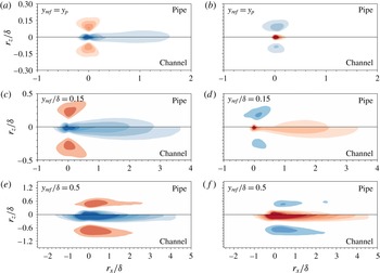
Figure 8 displays the wall-parallel planes of the conditional cross-correlations $R_{T_{I}u}$ at $y_{ref}/\unicode[STIX]{x1D6FF}=y_{p}/\unicode[STIX]{x1D6FF}$ , 0.15 and 0.5. At $y_{ref}=y_{p}$ (figure 8 a,b), where the turbulent inertia is zero due to the balance between acceleration and deceleration forces, $R_{T_{p}u}$ and $R_{T_{n}u}$ of the pipe and channel flows show the negative and positive values along $r_{z}=0$ , respectively, flanked on both sides by regions of opposite sign. The sign of both correlations indicates that the momentum source and sink are associated with the negative- $u$ regions. However, the negative- $u$ region associated with $T_{p}$ is elongated in the downstream, whereas the negative- $u$ region associated with $T_{n}$ is spatially compact in the vicinity of $T_{n}$ . Further away from the wall ( $y_{ref}/\unicode[STIX]{x1D6FF}=0.15$ and 0.5), the patterns of the correlations between the pipe and channel flows are noticeably different. The negative and positive regions of $R_{T_{I}u}$ increase along both the streamwise and spanwise directions, indicating that the low- and high-speed regions associated with $T_{p}$ and $T_{n}$ grow along the wall-normal distance. The negative (positive) values of $R_{T_{p}u}$ ( $R_{T_{n}u}$ ) in the pipe flow are shorter than those in the channel. These observations indicate two things: (i) the momentum source-like motions in the overlap region are associated with long low-speed structures, whereas the momentum sinks are related to short and narrow negative- $u$ regions. This result is consistent with the net force spectrum, which indicates that positive $\unicode[STIX]{x2202}\unicode[STIX]{x1D6F7}_{-uv}^{+}/\unicode[STIX]{x2202}y^{+}$ only appears at longer wavelengths $\unicode[STIX]{x1D706}_{x}>3\unicode[STIX]{x1D6FF}$ in the overlap region. (ii) The low-speed structures related to the accelerating motions are longer and wider in the channel flow compared to the pipe flow. In this manner the relatively high positive $\unicode[STIX]{x2202}\unicode[STIX]{x1D6F7}_{-uv}^{+}/\unicode[STIX]{x2202}y^{+}$ regions observed in the channel flow arise from these low-speed structures.

Figure 9.

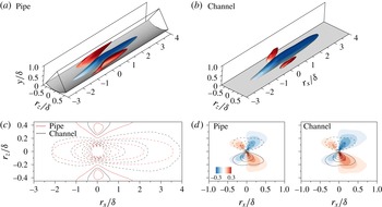
Conditional structures associated with the momentum source at $y/\unicode[STIX]{x1D6FF}=0.15$ . (a,b) Isosurfaces of $u^{+}|_{T_{p}}=-0.4$ (blue), $+0.2$ (red). (c,d) Conditionally averaged velocity fields in the $x{-}z$ plane ( $y/\unicode[STIX]{x1D6FF}=0.15$ ). (c) The line contour represents $u^{+}|_{T_{p}}$ range from $-0.2$ to $-1.0$ with an interval of $-0.2$ (dashed), and $u^{+}|_{T_{p}}=0.15$ , 0.3 (solid). (d) The filled contours represent $w^{+}|_{T_{p}}$ . The inserted line contours are $\unicode[STIX]{x1D714}_{y}^{+}|_{T_{p}}$ and their magnitudes range from $-0.025$ to 0.025 with an interval of 0.005; the solid (dashed) lines represent positive (negative) values.

To further examine the flow field around the momentum source, the conditionally averaged velocity is defined as

(3.6) $$\begin{eqnarray}\boldsymbol{u}|_{T_{p}}(r_{x},y,r_{z})=\langle \boldsymbol{u}(x+r_{x},y,z+r_{z})\,|\,E(x,y_{ref},z)\rangle ,\end{eqnarray}$$

where the event $E$ is $E(x,y_{ref},z)=\{u(x,y_{ref},z)<0~\& ~T(x,y_{ref},z)>1.5\unicode[STIX]{x1D70E}_{T}(y_{ref})\}$ . The reference wall-normal position is $y_{ref}/\unicode[STIX]{x1D6FF}=0.15$ . The negative- $u$ region is associated with the momentum source in the overlap region (figure 8). The negative- $u$ event is conditionally averaged with the turbulent inertia yielding a value more than 1.5 times its root mean square value. Figures 9(a,b) illustrate the isosurfaces of the conditional streamwise velocity fluctuation $u^{+}|_{T_{p}}$ . The negative- $u$ structure has long streamwise lengths, extending over $4\unicode[STIX]{x1D6FF}$ along the streamwise direction and relatively short positive- $u$ regions flanked on its both sides. Hence, the conditional structures shown here can be considered as LSMs associated with the momentum source in the overlap region. The high-speed structures of the pipe flow are distinct, whereas the low-speed structures of the channel flow in the upstream position are thicker than those of the pipe flow. These differences are apparent in the wall-parallel plane. The conditionally averaged streamwise velocity fluctuations in the $x$ – $z$ plane at $y/\unicode[STIX]{x1D6FF}=0.15$ are illustrated in figure 9(c). The high-speed regions appear at $r_{z}/\unicode[STIX]{x1D6FF}=\pm 0.4\unicode[STIX]{x1D6FF}$ and extend over $3\unicode[STIX]{x1D6FF}$ in the pipe flow ( $1\unicode[STIX]{x1D6FF}$ in the channel flow). In addition, the maximum strengths of $u^{+}|_{T_{p}}$ are 0.33 (pipe) and 0.25 (channel), whereas the minimum value is $u^{+}|_{T_{p}}=-2.7$ in both flows. The negative- $u$ regions converge for $r_{x}/\unicode[STIX]{x1D6FF}<0$ and diverge for $r_{x}/\unicode[STIX]{x1D6FF}>0$ . This trend is more prominent in the channel flow than in the pipe flow for $r_{x}/\unicode[STIX]{x1D6FF}>0$ because the high-speed regions in the pipe flow extend farther along the downstream direction, which restrict the spanwise size of the low-speed regions.

As mentioned earlier, the relatively strong momentum source in the overlap region of the channel flow is attributed to the contributions of the correlations between the spanwise velocity fluctuations and the wall-normal vorticity fluctuations $\langle -w\unicode[STIX]{x1D714}_{y}\rangle$ . Figure 9(d) shows $w^{+}|_{T_{p}}$ (filled contour) and $\unicode[STIX]{x1D714}_{y}^{+}|_{T_{p}}$ (line contour) in the $x$ – $z$ plane ( $y/\unicode[STIX]{x1D6FF}=0.15$ ). Two pairs of the positive- and negative- $w$ regions are observed in the downstream and upstream positions, respectively. The downstream pairs are broader in both the spanwise and downstream directions, with a higher magnitude; the maximum magnitude of the downstream pair is approximately 2.4 times that of the upstream one. Note that the conditionally averaged field conditioned on the momentum sink ( $T_{n}$ ) shows wider patterns of $w$ in the upstream direction (not shown here). The asymmetric patterns of the $w$ pairs indicate the acceleration (deceleration) effect in the presence of strong pairs in the downstream (upstream) direction. Although the strong downstream pair appears in both the pipe and channel flows, the downstream pair of the channel flow is wider and its maximum value is 1.2 times that of the pipe flow. Conversely, the $\unicode[STIX]{x1D714}_{y}^{+}|_{T_{p}}$ regions (line contours) are identical to one another. The second term ( $\langle -w\unicode[STIX]{x1D714}_{y}\rangle$ ) in (3.4) indicates that the intense spanwise velocity fluctuations in the channel flow contribute to strong momentum source-like motions. Since this term represents a body force associated with the change of size of eddies, the large-scale low-speed structures of the channel flow strongly modulate the small scales in the outer region compared to those of the pipe flow (cf. figure 7 b,d). Overall, relatively short and narrow low-speed structures in the pipe flow induce the weaker spanwise velocity fluctuations, and thus contribute to the weak momentum source in the overlap region compared to the channel flow.

3.4 Spanwise scale growth

The structural difference of LSAMs ( $\unicode[STIX]{x1D706}_{x}>3\unicode[STIX]{x1D6FF}$ ) between the pipe and channel flows causes a relatively lower acceleration effect in the pipe flow. One of the noticeable features is the intense positive- $u$ regions flanked on the low-speed structure in the pipe flow. Owing to these regions, the low-speed structures in the pipe flow are relatively short and narrow, leading to the weak spanwise velocity fluctuations. Hence, statistical analyses are valuable for comparing the spanwise scale of LSAMs in the outer region of internal flows. Although the spanwise scale growths of the pipe, channel and boundary layer flows were investigated in Monty et al. (Reference Monty, Stewart, Williams and Chong2007), they mainly focused on the difference between the internal flow (pipe/channel) and boundary layer. The aim of the present study is to explore the spanwise scale growth of the large scales that play a role in accelerating the mean flow. We use a similar expression of the conditional two-point correlation reported in Bailey & Smits (Reference Bailey and Smits2010). The conditional two-point correlation of the streamwise velocity fluctuations for large scales ( $\unicode[STIX]{x1D706}_{x}>3\unicode[STIX]{x1D6FF}$ ) is defined as

(3.7) $$\begin{eqnarray}R_{LS}(r_{x},y,r_{z};y_{ref})=\frac{\displaystyle \int _{0}^{k_{c}}C(k_{x},y,r_{z};y_{ref})\cos (k_{x}r_{x})+Q(k_{x},y,r_{z};y_{ref})\sin (k_{x}r_{x})\,\text{d}k_{x}}{\unicode[STIX]{x1D70E}_{u}(y_{ref})\unicode[STIX]{x1D70E}_{u}(y)},\end{eqnarray}$$

where $C(k_{x},y,r_{x};y_{ref})$ and $Q(k_{x},y,r_{z};y_{ref})$ are the coincident and quadrature spectral density functions of the cross-spectral density function, respectively. The cross-spectral density function ( $G$ ) is defined as

(3.8) $$\begin{eqnarray}G(k_{x},y,r_{z};y_{ref})=2\int _{-\infty }^{\infty }\langle \hat{u} ^{\ast }(k_{x},y_{ref},k_{z})\hat{u} (k_{x},y,k_{z})\rangle \text{e}^{\text{i}k_{z}r_{z}}\,\text{d}k_{z}.\end{eqnarray}$$

Here, $\hat{u}$ indicates the Fourier transform of the streamwise velocity fluctuations and * indicates a complex conjugate. The cutoff wavenumber $k_{c}$ is chosen as the streamwise wavelength greater than $3\unicode[STIX]{x1D6FF}$ (e.g. $\unicode[STIX]{x1D706}_{x}=2\unicode[STIX]{x03C0}/k_{c}>3\unicode[STIX]{x1D6FF}$ ). Similarly, the conditional two-point correlation of the streamwise velocity fluctuations for small scales ( $\unicode[STIX]{x1D706}_{x}<3\unicode[STIX]{x1D6FF}$ ) is defined as

(3.9) $$\begin{eqnarray}R_{SS}(r_{x},y,r_{z};y_{ref})=\frac{\displaystyle \int _{k_{c}}^{\infty }C(k_{x},y,r_{z};y_{ref})\cos (k_{x}r_{x})+Q(k_{x},y,r_{z};y_{ref})\sin (k_{x}r_{x})\,\text{d}k_{x}}{\unicode[STIX]{x1D70E}_{u}(y_{ref})\unicode[STIX]{x1D70E}_{u}(y)}.\end{eqnarray}$$

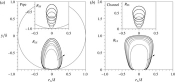
Figure 10 shows 0.05 contour line of $R_{LS}$ for a series of $y_{ref}$ in the cross-stream plane ( $r_{x}=0$ ). The inset represents the wall-normal variation of $R_{SS}$ . The spanwise scales of $R_{SS}$ also grow as $y_{ref}$ increases but their sizes are less than $0.3\unicode[STIX]{x1D6FF}$ which is significantly smaller than those of $R_{LS}$ . Above $y_{ref}/\unicode[STIX]{x1D6FF}>0.15$ , the contours of $R_{SS}$ are detached from the wall, whereas those of $R_{LS}$ are attached from the wall, except for the $R_{LS}$ of the pipe flow at $y_{ref}/\unicode[STIX]{x1D6FF}=0.5$ . The contours of $R_{LS}$ penetrate into the core and extend down to the wall in both flows. However, comparison of figure 10(a,b) indicates that the upper parts ( $y>y_{ref}$ ) of each $R_{LS}$ in the channel flow are significantly larger than those in the pipe flow. As $y_{ref}$ increases, in particular, the upper part of $R_{LS}$ in the channel flow becomes broader than the lower part. The size of LSMs in the pipe flow is significantly restricted, even in the overlap region, and the restriction becomes severe as the size of the structures ( $y_{ref}$ ) increases.

Figure 10.

The 0.05-contours of $R_{LS}$ ; (a) pipe, (b) channel. The reference positions are $y_{ref}^{+}=y_{p}^{+}$ , $0.15\unicode[STIX]{x1D6FF}^{+}$ , $0.2\unicode[STIX]{x1D6FF}^{+}$ , $0.3\unicode[STIX]{x1D6FF}^{+}$ , $0.4\unicode[STIX]{x1D6FF}^{+}$ and $0.5\unicode[STIX]{x1D6FF}^{+}$ (from thinner to thicker solid line). The inset represents 0.05-contours of  $R_{SS}$ .

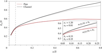
To further investigate this difference, the spanwise length scale ( $L_{z}$ ) is measured; $L_{z}$ is the distance between the points where the spanwise correlation crosses at $R_{LS}(r_{x}=0,y_{ref},r_{z})=0.05$ (Monty et al. Reference Monty, Stewart, Williams and Chong2007). This quantity represents the average spanwise scale of LSMs. Figure 11 shows the wall-normal variation of $L_{z}$ in the pipe and channel flows. The profiles of $L_{z}$ are almost identical below $y^{+}\approx y_{p}^{+}$ (vertical dashed line), but a discrepancy arises above $y^{+}\approx y_{p}^{+}$ ; the growth rate of the pipe flow is relatively lower than that of the channel flow. The discrepancy becomes greater as the wall-normal location is close to the centre. Monty et al. (Reference Monty, Stewart, Williams and Chong2007) compared the growth rate by fitting the data linearly since the spanwise length scale increases linearly (Tomkins & Adrian Reference Tomkins and Adrian2003). The profiles of $L_{z}$ within the range $y_{p}^{+}<y^{+}<0.2\unicode[STIX]{x1D6FF}^{+}$ are fitted; the slopes are $a_{1}=1.20$ and $a_{2}=0.81$ for the channel and pipe flows, respectively. The higher slope in the channel flow indicates that the coherence of LSMs is preserved well beyond the overlap region. In other words, a lower population of relatively smaller scales is present in the channel flow compared to that in the pipe flow. Lee et al. (Reference Lee, Ahn and Sung2015) addressed that the population density of very long streaks in the pipe flow decreases significantly while that of relatively short streaks increases in the core region, supporting the breakdown of large-scale structures in the pipe flow. This breakdown could be enhanced at higher Reynolds number pipe flows, leading to the formation of two outer sites ( $\unicode[STIX]{x1D706}_{z}/\unicode[STIX]{x1D6FF}\approx 0.6$ and 1.3) in the premultiplied spanwise energy spectrum of the pipe flow at $\mathit{Re}_{\unicode[STIX]{x1D70F}}\approx 3000$ (Ahn et al. Reference Ahn, Lee, Lee, Kang and Sung2015). Note that one outer site ( $\unicode[STIX]{x1D706}_{z}/\unicode[STIX]{x1D6FF}\approx 1.0$ ) was observed in the channel flow at $\mathit{Re}_{\unicode[STIX]{x1D70F}}\approx 5200$ (Lee & Moser Reference Lee and Moser2015).

To verify the effect of the pipe curvature to the spanwise scale growth, we modify the wall-normal variation of $R_{LS}$ . Chung et al. (Reference Chung, Marusic, Monty, Vallikivi and Smits2015) proposed a simple modification to the upper limit of the two-dimensional spectrum by a factor ( $1-\unicode[STIX]{x1D6FD}y/\unicode[STIX]{x1D6FF}$ ), to scale the second-order structure function in the pipe flow. This reflects the spatial hindrance exerted by the pipe circumference as $y$ goes to the centre. Hence, in order to compensate the decrease of the spanwise scale, the wall-normal variation of $R_{LS}$ in the pipe flow is multiplied by a factor ( $1+\unicode[STIX]{x1D6FD}y/\unicode[STIX]{x1D6FF}$ ). The modified spanwise scale growth of $R_{LS}$ is shown in the grey line in figure 11. Here, $\unicode[STIX]{x1D6FD}$ is the ratio between the slopes of the pipe and channel flows ( $a_{2}/a_{1}=0.675$ ). Interestingly, the modified scale growth (grey line) collapses well up to $y/\unicode[STIX]{x1D6FF}\approx 0.25$ , indicating that the spanwise scale of the LSMs in the pipe flow is influenced by its curvature. Owing to the pipe curvature, the size of the LSMs could be hindered by other LSMs that are located in the neighbouring wall. Above $y/\unicode[STIX]{x1D6FF}>0.25$ , however, the discrepancy becomes prominent as $y$ increases due to the different scale growth in the wake region. Beyond the overlap region, $L_{z}$ of the pipe flow approaches a new slope and the growth rate flattens to the centre. In figure 10, the lower part of $R_{LS}$ at $y_{ref}/\unicode[STIX]{x1D6FF}=0.5$ in the pipe flow is detached from the wall while that of the channel flow remains attached.

Figure 11.

Wall-normal variation of the spanwise scale $L_{z}$ ; pipe (red) and channel (black). The inserted vertical dashed line marks $y^{+}=y_{p}^{+}$ . In the inset, the dashed lines mark a liner fit in the range $y_{p}^{+}<y^{+}<0.2\unicode[STIX]{x1D6FF}^{+}$ . The grey line represents the modified spanwise scale growth of the pipe flow by a factor ( $1+\unicode[STIX]{x1D6FD}y/\unicode[STIX]{x1D6FF}$ ), where $\unicode[STIX]{x1D6FD}=0.675$ is a ratio between the slopes of fitted data $(a_{2}/a_{1})$ .